Deep Learning

1. Gradient descent variants

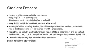
2. Gradient Descent
• current position → → → initial parameters
baby step → → → learning rate
direction → → → partial derivative (gradient)
• Why do We Need the Gradient Descent Algorithm?
• In many machine learning models, our ultimate goal is to find the best parameter
values that reduce the cost associated with the predictions.
• To do this, we initially start with random values of these parameters and try to find
the optimal ones. To find the optimal values, we use the gradient descent algorithm.
• Gradients are nothing but a vector whose entries are
partial derivatives of a function.

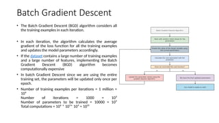
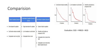
4. Batch Gradient Descent
• The Batch Gradient Descent (BGD) algorithm considers all
the training examples in each iteration.
• In each iteration, the algorithm calculates the average
gradient of the loss function for all the training examples
and updates the model parameters accordingly.
• If the dataset contains a large number of training examples
and a large number of features, implementing the Batch
Gradient Descent (BGD) algorithm becomes
computationally expensive
• In batch Gradient Descent since we are using the entire
training set, the parameters will be updated only once per
epoch.
• Number of training examples per iterations = 1 million =
10⁶
Number of iterations = 1000 = 10³
Number of parameters to be trained = 10000 = 10⁴
Total computations = 10⁶ * 10³* 10⁴ = 10¹³

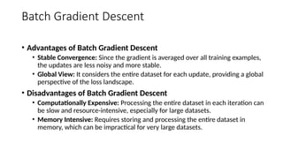
5. Batch Gradient Descent
• Advantages of Batch Gradient Descent
• Stable Convergence: Since the gradient is averaged over all training examples,
the updates are less noisy and more stable.
• Global View: It considers the entire dataset for each update, providing a global
perspective of the loss landscape.
• Disadvantages of Batch Gradient Descent
• Computationally Expensive: Processing the entire dataset in each iteration can
be slow and resource-intensive, especially for large datasets.
• Memory Intensive: Requires storing and processing the entire dataset in
memory, which can be impractical for very large datasets.

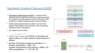
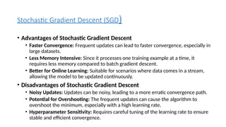
6. Stochastic Gradient Descent (SGD)
• Stochastic Gradient Descent (SGD) is a variant of the
gradient descent algorithm where the model parameters
are updated using the gradient of the loss function with
respect to a single training example at each iteration.
• Unlike batch gradient descent, which uses the entire
dataset, SGD updates the parameters more frequently,
leading to faster convergence.
• The update rule for SGD is:
• In the case of SGD, there will be ‘m’ iterations per
epoch, where ‘m’ is the number of observations in a
dataset.
• Number of training examples per iterations = 1
Number of iterations = 1000 = 10³
Number of parameters to be trained = 10000 = 10⁴
Total computations = 1 * 10³*10⁴=10⁷

8. Stochastic Gradient Descent (SGD)
• Advantages of Stochastic Gradient Descent
• Faster Convergence: Frequent updates can lead to faster convergence, especially in
large datasets.
• Less Memory Intensive: Since it processes one training example at a time, it
requires less memory compared to batch gradient descent.
• Better for Online Learning: Suitable for scenarios where data comes in a stream,
allowing the model to be updated continuously.
• Disadvantages of Stochastic Gradient Descent
• Noisy Updates: Updates can be noisy, leading to a more erratic convergence path.
• Potential for Overshooting: The frequent updates can cause the algorithm to
overshoot the minimum, especially with a high learning rate.
• Hyperparameter Sensitivity: Requires careful tuning of the learning rate to ensure
stable and efficient convergence.

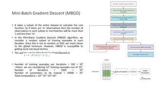
11. Mini-Batch Gradient Descent (MBGD)
• It takes a subset of the entire dataset to calculate the cost
function. So if there are ‘m’ observations then the number of
observations in each subset or mini-batches will be more than
1 and less than ‘m’.
• in the Mini-Batch Gradient Descent (MBGD) algorithm, we
consider a random subset of training examples in each
iteration. Since this is not as random as SGD, we reach closer
to the global minimum. However, MBGD is susceptible to
getting stuck into local minima.
• The update rule for Mini-Batch Gradient Descent is:
• Number of training examples per iterations = 100 = 10²
→Here, we are considering 10² training examples out of 10⁶.
Number of iterations = 1000 = 10³
Number of parameters to be trained = 10000 = 10⁴
Total computations = 10²*10³*10⁴=10⁹

12. Mini-Batch Gradient Descent (MBGD)
• Advantages of Mini-Batch Gradient Descent
• Faster Convergence: By using mini-batches, it achieves a balance between the noisy updates of SGD and
the stable updates of Batch Gradient Descent, often leading to faster convergence.
• Reduced Memory Usage: Requires less memory than Batch Gradient Descent as it only needs to store a
mini-batch at a time.
• Efficient Computation: Allows for efficient use of hardware optimizations and parallel processing, making
it suitable for large datasets.
• Disadvantages of Mini-Batch Gradient Descent
• Complexity in Tuning: Requires careful tuning of the mini-batch size and learning rate to ensure optimal
performance.
• Less Stable than Batch GD: While more stable than SGD, it can still be less stable than Batch Gradient
Descent, especially if the mini-batch size is too small.
• Potential for Suboptimal Mini-Batch Sizes: Selecting an inappropriate mini-batch size can lead to
suboptimal performance and convergence issues.
• Used in Intense learning

13. Comparision
Evaluation: SGD > MBGD > BGD

14. Momentum-Based Gradient Descent

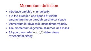
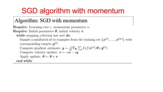
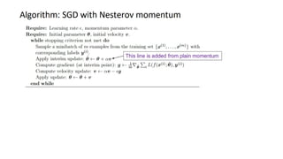
15. Momentum-Based Gradient Descent
• The problem with Gradient Descent is that the weight update
at a moment (t) is governed by the learning rate and gradient
at that moment only.
• It doesn’t take into account the past steps taken while
traversing the cost space.
• It leads to the following problems.
• The gradient of the cost function at saddle points( plateau) is
negligible or zero, which in turn leads to small or no weight updates.
Hence, the network becomes stagnant, and learning stops
• The path followed by Gradient Descent is very jittery even when
operating with mini-batch mode
• To account for the momentum, we can use a moving average
over the past gradients.

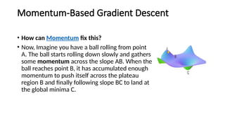
16. Momentum-Based Gradient Descent
• How can Momentum fix this?
• Now, Imagine you have a ball rolling from point
A. The ball starts rolling down slowly and gathers
some momentum across the slope AB. When the
ball reaches point B, it has accumulated enough
momentum to push itself across the plateau
region B and finally following slope BC to land at
the global minima C.

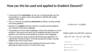
19. How can this be used and applied to Gradient Descent?
• To account for the momentum, we can use a moving average over the
past gradients. In regions where the gradient is high like AB, weight
updates will be large.
• Thus, in a way we are gathering momentum by taking a moving average
over these gradients.
• But there is a problem with this method, it considers all the gradients
over iterations with equal weightage.
• The gradient at t=0 has equal weightage as that of the gradient at current
iteration t. We need to use some sort of weighted average of the past
gradients such that the recent gradients are given more weightage.
• This can be done by using an Exponential Moving Average(EMA). An
exponential moving average is a moving average that assigns a greater
weight on the most recent values.
• Higher β will accommodate more gradients from the past. Hence,
generally, β is kept around 0.9 in most of the cases.
Weight update rule with EMA is given as:
vt​
=Beta*v(t 1)​
+
− η∇J(θt​
)

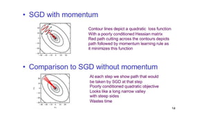
22. • Overcome saddle point issue
• Using momentum with gradient descent, gradients from the past will push the cost further to move
around a saddle point.
• Overcome learning rate issue
• Case 1: When all the past gradients have the same sign
• The summation term will become large and we will take large steps while updating the weights. Along the curve BC,
even if the learning rate is low, all the gradients along the curve will have the same direction(sign) thus increasing
the momentum and accelerating the descent.
• Case 2: when some of the gradients have +ve sign whereas others have –ve
• The summation term will become small and weight updates will be small. If the learning rate is high, the gradient at
each iteration around the valley C will alter its sign between +ve and -ve and after few oscillations, the sum of past
gradients will become small. Thus, making small updates in the weights from there on and damping the oscillations.
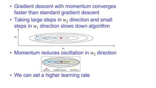
• Gradient Descent with Momentum takes small steps in directions where the gradients oscillate and take
large steps along the direction where the past gradients have the same direction(same sign).
• By adding a momentum term in the gradient descent, gradients accumulated from past iterations will
push the cost further to move around a saddle point even when the current gradient is negligible or zero.

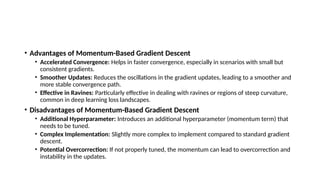
24. • Advantages of Momentum-Based Gradient Descent
• Accelerated Convergence: Helps in faster convergence, especially in scenarios with small but
consistent gradients.
• Smoother Updates: Reduces the oscillations in the gradient updates, leading to a smoother and
more stable convergence path.
• Effective in Ravines: Particularly effective in dealing with ravines or regions of steep curvature,
common in deep learning loss landscapes.
• Disadvantages of Momentum-Based Gradient Descent
• Additional Hyperparameter: Introduces an additional hyperparameter (momentum term) that
needs to be tuned.
• Complex Implementation: Slightly more complex to implement compared to standard gradient
descent.
• Potential Overcorrection: If not properly tuned, the momentum can lead to overcorrection and
instability in the updates.

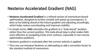
25. Nesterov Accelerated Gradient (NAG)
• Nesterov Accelerated Gradient is a refined version of momentum-based
optimization, designed to further smooth and speed up convergence. It
does so by looking ahead at the future gradient and adjusting accordingly,
which helps reduce overshooting and improves stability.
• In simple terms, NAG calculates the gradient at a “look-ahead” position
rather than the current position. This look-ahead step is what makes NAG
more effective at navigating tricky error surfaces, especially in non-convex
optimization problems.
• Nesterov gradient is evaluated after the current velocity is applied.
• Thus one can interpret Nesterov as attempting to add a correction factor to
the standard method of momentum

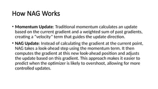
26. How NAG Works
• Momentum Update: Traditional momentum calculates an update
based on the current gradient and a weighted sum of past gradients,
creating a “velocity” term that guides the update direction.
• NAG Update: Instead of calculating the gradient at the current point,
NAG takes a look-ahead step using the momentum term. It then
computes the gradient at this new look-ahead position and adjusts
the update based on this gradient. This approach makes it easier to
predict when the optimizer is likely to overshoot, allowing for more
controlled updates.

29. Advantages of NAG
• Reduced Oscillations: By peeking ahead, NAG reduces oscillations
around the minimum, which can be especially useful in error surfaces
with multiple peaks and valleys.
• Faster Convergence: NAG often converges faster than simple
momentum-based methods because it reduces unnecessary steps
around the optimum.

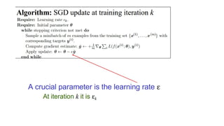
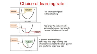
30. • Learning rate: most difficult hyperparamer to set
• It significantly affects model performance
• Cost is highly sensitive to some directions in parameter space and
insensitive to others – Momentum helps but introduces another
hyper parameter – Is there another way?
• If direction of sensitivity is axis aligned, separate learning rate for each
parameter and adjust them throughput learning

32. Adaptive Learning Rate Methods
• Adaptive learning rate methods adjust the learning rate during the
optimization process.
• Unlike traditional methods where the learning rate is fixed, adaptive
methods change the learning rate based on certain criteria, often related to
gradient information.
• This adjustment helps the algorithm converge faster and more reliably.
• Adaptive learning rates offer many advantages:
• Efficiency: Training can be faster because it adjusts the learning rate dynamically.
• Stability: Helps prevent the algorithm from overshooting the minimum.
• Adaptability: Works well with different types of data and does not require extensive
tuning.

33. Adaptive Learning Rate Methods
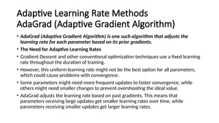
AdaGrad (Adaptive Gradient Algorithm)
• AdaGrad (Adaptive Gradient Algorithm) is one such algorithm that adjusts the
learning rate for each parameter based on its prior gradients.
• The Need for Adaptive Learning Rates
• Gradient Descent and other conventional optimization techniques use a fixed learning
rate throughout the duration of training.
• However, this uniform learning rate might not be the best option for all parameters,
which could cause problems with convergence.
• Some parameters might need more frequent updates to faster convergence, while
others might need smaller changes to prevent overshooting the ideal value.
• AdaGrad adjusts the learning rate based on past gradients. This means that
parameters receiving large updates get smaller learning rates over time, while
parameters receiving smaller updates get larger learning rates.

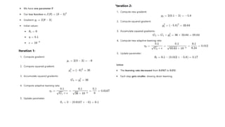
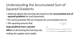
34. Understanding the Accumulated Sum of
Squared Gradients
• AdaGrad adjusts the learning rate based on the accumulated sum of
squared gradients for each parameter.
• For each parameter θ(i),we compute the accumulated sum as:
• The squaring ensures that
large gradients have a greater
effect on decreasing the learning rate,
making the update more stable.

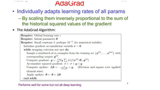
35. How AdaGrad Works
• AdaGrad’s main principle is to scale the learning rate for
each parameter according to the total of squared
gradients observed during training.
• The steps of the algorithm are as follows:
• Step 1: Initialize variables
• Initialize the parameters θ and a small constant ϵ to
avoid division by zero.
• Initialize the sum of squared gradients variable G with
zeros, which has the same shape as θ.
• Step 2: Calculate gradients
• Compute the gradient of the loss function with respect
to each parameter, θJ(θ)
∇
• Step 3: Accumulate squared gradients
• Update the sum of squared gradients G for each
parameter i: G[i] += ( θJ(θ[i]))²
∇
• Step 4: Update parameters

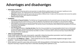
38. Advantages and disadvantges
• Advantages of AdaGrad
• AdaGrad adjusts the learning rate for each parameter to enable effective updates based on the parameter’s significance to the
optimization process. This method lessens the requirement for manual adjustment of learning rates.
• Robustness: AdaGrad does well with sparse data and variables of different sizes. It makes sure that parameters that receive few updates
get higher learning rates, which speeds up convergence.
• Robust to Feature Scaling
• Limitations
• Accumulation of Squared Gradients: The AdaGrad sum of squared gradients has the potential to grow very big over time, which could
cause the learning rate to drop too low. As a result, the algorithm may experience slow convergence or even premature stalling.
• Lack of Control: AdaGrad does not provide fine-grained control over the learning rates of particular parameters because it globally
accumulates squared gradients for all parameters. This may be an issue in circumstances where different learning speeds are necessary.
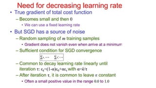
Improvements and Variations
• Learning Rate Decay
One of its biggest limitations is learning rate decay. Over time, the accumulated sum of squared gradients (the Gt​term in the formula)
can grow quite large, causing the learning rate to shrink too much. This leads to a situation where the model stops learning altogether
because the updates become so tiny that they have little to no effect. In scenarios where continuous learning is required (like deep
learning), this can be a dealbreaker.
• When to Avoid AdaGrad
If your model needs to learn over many epochs, especially in deep learning where parameters need to be updated
continuously, AdaGrad’s shrinking learning rate can become a bottleneck.
• Use optimizers like RMSProp or Adam — which tackle this issue by using exponentially weighted averages of past
gradients — tend to perform better in these cases.
• While AdaGrad is great for sparse data and scenarios with strong gradients in the beginning, its performance drops when
long-term learning is required. Keep that in mind when deciding which optimizer to use.

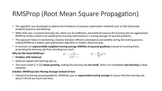
39. RMSProp (Root Mean Square Propagation)
• The algorithm was developed to address the limitations of previous optimization methods such as SGD (Stochastic
Gradient Descent) and AdaGrad.
• While SGD uses a constant learning rate, which can be inefficient, and AdaGrad reduces the learning rate too aggressively,
RMSProp strikes a balance by adapting the learning rates based on a moving average of squared gradients.
• This approach helps in maintaining a balance between efficient convergence and stability during the training process,
making RMSProp a widely used optimization algorithm in modern deep learning.
• It maintains an exponentially weighted moving average (EWMA) of squared gradients instead of summing them,
preventing the learning rate from shrinking too much.
Why Do We Need RMSProp?
• Problem with AdaGrad:
• AdaGrad updates the learning rate as:
• The issue is that G_t^{(i)} keeps growing, making the learning rate too small, which can completely stop learning in deep
networks.
Solution: RMSProp Uses Moving Average Instead of Sum
• Instead of summing squared gradients, RMSProp uses an exponential moving average to ensure that the learning rate
doesn’t shrink too much over time.

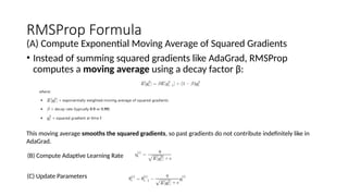
40. RMSProp Formula
(A) Compute Exponential Moving Average of Squared Gradients
• Instead of summing squared gradients like AdaGrad, RMSProp
computes a moving average using a decay factor β:
This moving average smooths the squared gradients, so past gradients do not contribute indefinitely like in
AdaGrad.
(B) Compute Adaptive Learning Rate
(C) Update Parameters

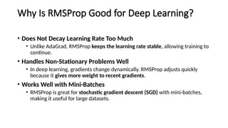
43. Why Is RMSProp Good for Deep Learning?
• Does Not Decay Learning Rate Too Much
• Unlike AdaGrad, RMSProp keeps the learning rate stable, allowing training to
continue.
• Handles Non-Stationary Problems Well
• In deep learning, gradients change dynamically. RMSProp adjusts quickly
because it gives more weight to recent gradients.
• Works Well with Mini-Batches
• RMSProp is great for stochastic gradient descent (SGD) with mini-batches,
making it useful for large datasets.

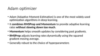
44. Adam optimizer
• Adam (Adaptive Moment Estimation) is one of the most widely used
optimization algorithms in deep learning.
• It combines RMSProp and Momentum to provide adaptive learning
rates without slowing down too much.
• Momentum helps smooth updates by considering past gradients.
• RMSProp adjusts learning rates dynamically using the squared
gradient moving average.
• Generally robust to the choice of hyperparameters

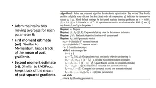
45. • Adam maintains two
moving averages for each
parameter θ:
• First moment estimate
(mt​
): Similar to
Momentum, keeps track
of the mean of past
gradients.
• Second moment estimate
(vt​
): Similar to RMSProp,
keeps track of the mean
of past squared gradients.

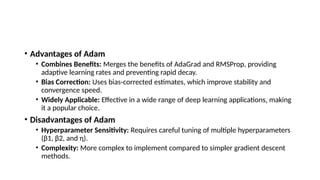
46. • Advantages of Adam
• Combines Benefits: Merges the benefits of AdaGrad and RMSProp, providing
adaptive learning rates and preventing rapid decay.
• Bias Correction: Uses bias-corrected estimates, which improve stability and
convergence speed.
• Widely Applicable: Effective in a wide range of deep learning applications, making
it a popular choice.
• Disadvantages of Adam
• Hyperparameter Sensitivity: Requires careful tuning of multiple hyperparameters
(β1​
, β2​
, and η).
• Complexity: More complex to implement compared to simpler gradient descent
methods.

47. Challenges and Improvements in Adam
• Problems with Adam
• Non-convergence Issues
• Adam sometimes struggles with generalization, leading to poor test performance.
• Sharp Minima Problem
• Adam may converge to sharp minima, which leads to poor generalization.
• Hyperparameter Sensitivity
• Adam is sensitive to the choice of β1,β2, requiring fine-tuning.
• Improved Variants of Adam
• AMSGrad
• Fixes the non-convergence issue by modifying the second moment update.
• Formula: vt=max⁡
(vt−1,vt)
• Ensures the learning rate does not increase unexpectedly.
• AdamW
• Introduces weight decay, improving generalization.
• Used in transformers and deep networks.

48. • Understanding Deep Learning Optimizers: Momentum, AdaGrad,
RMSProp & Adam | Towards Data Science

49. Choosing right optimizer

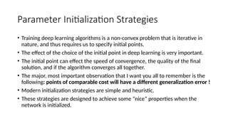
50. Parameter Initialization Strategies
• Training deep learning algorithms is a non-convex problem that is iterative in
nature, and thus requires us to specify initial points.
• The effect of the choice of the initial point in deep learning is very important.
• The initial point can effect the speed of convergence, the quality of the final
solution, and if the algorithm converges all together.
• The major, most important observation that I want you all to remember is the
following: points of comparable cost will have a different generalization error !
• Modern initialization strategies are simple and heuristic.
• These strategies are designed to achieve some ”nice” properties when the
network is initialized.

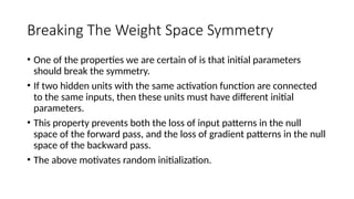
51. Breaking The Weight Space Symmetry
• One of the properties we are certain of is that initial parameters
should break the symmetry.
• If two hidden units with the same activation function are connected
to the same inputs, then these units must have different initial
parameters.
• This property prevents both the loss of input patterns in the null
space of the forward pass, and the loss of gradient patterns in the null
space of the backward pass.
• The above motivates random initialization.

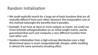
52. Random Initialization
• We could explicitly search for a large set of basis functions that are all
mutually different from each other. However, the computation cost of
this method outweighs the benefits that it provides.
• Example: If we have at most as many outputs as inputs, we could use
Gram-Schmidt orthogonalization on an initial weight matrix, and be
guaranteed that each unit computes a very different function from
each other unit.
• Random Initialization from a high entropy distribution over a high
dimensional space is much computationally cheaper, while resulting
in almost the same symmetry breaking effect

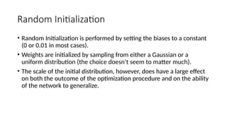
53. Random Initialization
• Random Initialization is performed by setting the biases to a constant
(0 or 0.01 in most cases).
• Weights are initialized by sampling from either a Gaussian or a
uniform distribution (the choice doesn’t seem to matter much).
• The scale of the initial distribution, however, does have a large effect
on both the outcome of the optimization procedure and on the ability
of the network to generalize.

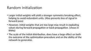
54. Random Initialization
• Larger initial weights will yield a stronger symmetry breaking effect,
helping to avoid redundant units. (Also prevents loss of signal in
forward pass)
• However, initial weights that are too large may result in exploding
values during forward propagation or back-propagation. (choas in
RNNs)
• The scale of the initial distribution, does have a large effect on both
the outcome of the optimization procedure and on the ability of the
network to generalize.

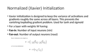
55. Normalized (Xavier) Initialization
• Xavier initialization is designed to keep the variance of activations and
gradients roughly the same across all layers. This prevents the
vanishing/exploding gradient problem. Used for tanh and sigmoid
• For a layer with weights W having:
• Fan-in: Number of input neurons (nin)
• Fan-out: Number of output neurons (nout)

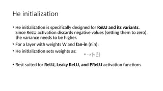
56. He initialization
• He initialization is specifically designed for ReLU and its variants.
Since ReLU activation discards negative values (setting them to zero),
the variance needs to be higher.
• For a layer with weights W and fan-in (nin​
):
• He initialization sets weights as:
• Best suited for ReLU, Leaky ReLU, and PReLU activation functions

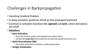
57. Challenges in Backpropagation
• Vanishing Gradient Problem
• In deep networks, gradients shrink as they propagate backward.
• Common in activation functions like sigmoid and tanh, where derivatives
are small.
• Solutions:
• ReLU Activation:
• ReLU f(x)=max⁡
(0,x) avoids small gradients for positive inputs.
• Variants like Leaky ReLU (f(x)=max⁡
(0.01x,x)) help when gradients become zero.
• Batch Normalization (BN):
• Normalizes activations to maintain a stable gradient flow.
• Weight Initialization

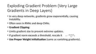
58. Exploding Gradient Problem (Very Large
Gradients in Deep Layers)
• In very deep networks, gradients grow exponentially, causing
instability.
• Often seen in RNNs and deep CNNs.
• Gradient Clipping:
• Limits gradient size to prevent extreme updates.
• If gradient norm exceeds a threshold, rescale it
• Use Proper Weight Initialization (same as vanishing gradients).

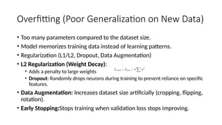
59. Overfitting (Poor Generalization on New Data)
• Too many parameters compared to the dataset size.
• Model memorizes training data instead of learning patterns.
• Regularization (L1/L2, Dropout, Data Augmentation)
• L2 Regularization (Weight Decay):
• Adds a penalty to large weights
• Dropout: Randomly drops neurons during training to prevent reliance on specific
features.
• Data Augmentation: Increases dataset size artificially (cropping, flipping,
rotation).
• Early Stopping:Stops training when validation loss stops improving.

60. Slow Convergence (Training Takes Too Long)
• Poor learning rate, bad weight initialization, lack of momentum.
• Use Momentum-Based Optimizers
• SGD with Momentum,ADAM

61. Saddle Points & Local Minima
• Gradient becomes zero in flat regions.
• The optimizer gets stuck.
• Use Adam Optimizer