Gradient Descent Batch Gradient Descent.pptx

Module 1 : : Overview of Machine Learning
1.1 The Motivation & Applications of Machine Learning
1.2 Learning Associations, Classification, Regression
1.3 Supervised Learning
1.5 Gradient Descent: Batch Gradient Descent, Stochastic Gradient
Descent
BEEE410L- MACHINE LEARNING
1.4 Unsupervised Learning; Reinforcement Learning;
1.6 Data Preprocessing
1.7 Under fitting and Overfitting issues.

1.5 Gradient Descent: Batch Gradient Descent, Stochastic
Gradient Descent
Gradient Descent
• .
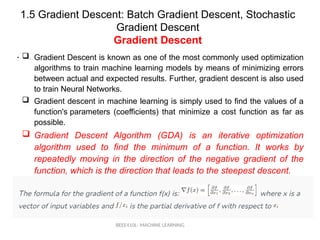
 Gradient Descent is known as one of the most commonly used optimization
algorithms to train machine learning models by means of minimizing errors
between actual and expected results. Further, gradient descent is also used
to train Neural Networks.
 Gradient descent in machine learning is simply used to find the values of a
function's parameters (coefficients) that minimize a cost function as far as
possible.
 Gradient Descent Algorithm (GDA) is an iterative optimization
algorithm used to find the minimum of a function. It works by
repeatedly moving in the direction of the negative gradient of the
function, which is the direction that leads to the steepest descent.

Gradient Descent
Gradient Descent
• .
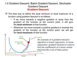
 The best way to define the local minimum or local maximum of a
function using gradient descent is as follows:
• If we move towards a negative gradient or away from the
gradient of the function at the current point, it will give
the local minimum of that function.
• Whenever we move towards a positive gradient or towards the
gradient of the function at the current point, we will get
the local maximum of that function
An example of a gradient descent
algorithm is linear regression. In linear
regression, gradient descent is used to
find the coefficients of a linear model
that best fits a set of data points.

Gradient Descent
Gradient Descent
• .
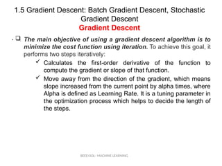
 The main objective of using a gradient descent algorithm is to
minimize the cost function using iteration. To achieve this goal, it
performs two steps iteratively:
 Calculates the first-order derivative of the function to
compute the gradient or slope of that function.
 Move away from the direction of the gradient, which means
slope increased from the current point by alpha times, where
Alpha is defined as Learning Rate. It is a tuning parameter in
the optimization process which helps to decide the length of
the steps.

Gradient Descent
cost function
• .
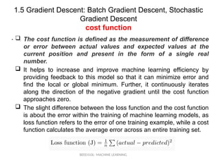
 The cost function is defined as the measurement of difference
or error between actual values and expected values at the
current position and present in the form of a single real
number.
 It helps to increase and improve machine learning efficiency by
providing feedback to this model so that it can minimize error and
find the local or global minimum. Further, it continuously iterates
along the direction of the negative gradient until the cost function
approaches zero.
 The slight difference between the loss function and the cost function
is about the error within the training of machine learning models, as
loss function refers to the error of one training example, while a cost
function calculates the average error across an entire training set.

Gradient Descent
Working of Gradient Descent
• .
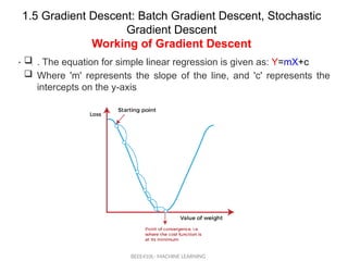
 . The equation for simple linear regression is given as: Y=mX+c
 Where 'm' represents the slope of the line, and 'c' represents the
intercepts on the y-axis

Gradient Descent
• .
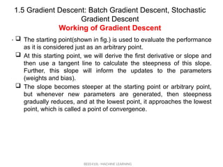
 The starting point(shown in fig.) is used to evaluate the performance
as it is considered just as an arbitrary point.
 At this starting point, we will derive the first derivative or slope and
then use a tangent line to calculate the steepness of this slope.
Further, this slope will inform the updates to the parameters
(weights and bias).
 The slope becomes steeper at the starting point or arbitrary point,
but whenever new parameters are generated, then steepness
gradually reduces, and at the lowest point, it approaches the lowest
point, which is called a point of convergence.

Gradient Descent
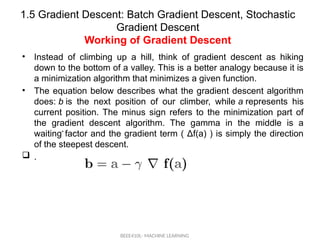
• Instead of climbing up a hill, think of gradient descent as hiking
down to the bottom of a valley. This is a better analogy because it is
a minimization algorithm that minimizes a given function.
• The equation below describes what the gradient descent algorithm
does: b is the next position of our climber, while a represents his
current position. The minus sign refers to the minimization part of
the gradient descent algorithm. The gamma in the middle is a
waiting factor and the gradient term ( Δf(a) ) is simply the direction
of the steepest descent.
 .
• .

1.5 Gradient Descent: Batch Gradient Descent,
Stochastic Gradient Descent
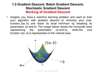
• Imagine you have a machine learning problem and want to train
your algorithm with gradient descent to minimize your cost-
function J(w, b) and reach its local minimum by tweaking its
parameters (w and b). The image below shows the horizontal axes
representing the parameters (w and b), while the cost
function J(w, b) is represented on the vertical axes.
• .

Learning Rate
• .
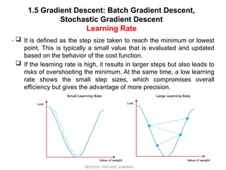
 It is defined as the step size taken to reach the minimum or lowest
point. This is typically a small value that is evaluated and updated
based on the behavior of the cost function.
 If the learning rate is high, it results in larger steps but also leads to
risks of overshooting the minimum. At the same time, a low learning
rate shows the small step sizes, which compromises overall
efficiency but gives the advantage of more precision.

How to Solve Gradient Descent Challenges
• .
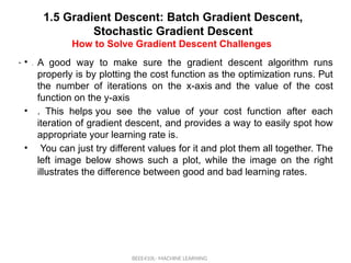
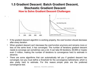
• A good way to make sure the gradient descent algorithm runs
properly is by plotting the cost function as the optimization runs. Put
the number of iterations on the x-axis and the value of the cost
function on the y-axis
• . This helps you see the value of your cost function after each
iteration of gradient descent, and provides a way to easily spot how
appropriate your learning rate is.
• You can just try different values for it and plot them all together. The
left image below shows such a plot, while the image on the right
illustrates the difference between good and bad learning rates.

How to Solve Gradient Descent Challenges
• .
• If the gradient descent algorithm is working properly, the cost function should decrease
after every iteration.
• When gradient descent can’t decrease the cost-function anymore and remains more or
less on the same level, it has converged. The number of iterations gradient descent
needs to converge can sometimes vary a lot. It can take 50 iterations, 60,000 or maybe
even 3 million, making the number of iterations to convergence hard to estimate in
advance.
• There are some algorithms that can automatically tell you if gradient descent has
converged, but you must define a threshold for the convergence beforehand, which is
also pretty hard to estimate. For this reason, simple plots are the preferred
convergence test.

Types of Gradient Descent
• .
 Based on the error in various training models, the Gradient Descent
learning algorithm can be divided into Batch gradient descent,
stochastic gradient descent, and mini-batch gradient descent.
1. Batch gradient descent
 Batch gradient descent (BGD) is used to find the error for each point
in the training set and update the model after evaluating all training
examples. This procedure is known as the training epoch.
 In simple words, it is a greedy approach where we have to sum over
all examples for each update.
Advantages of Batch gradient descent:
 It produces stable gradient descent convergence.
 It is Computationally efficient as all resources are used for all
training samples.

• .
2.stochastic descent
 Stochastic gradient descent (SGD) is a type of gradient descent that
runs one training example per iteration. Or in other words, it
processes a training epoch for each example within a dataset and
updates each training example's parameters one at a time. As it
requires only one training example at a time, hence it is easier to
store in allocated memory. However, it shows some computational
efficiency losses in comparison to batch gradient systems as it
shows frequent updates that require more detail and speed.
 Further, due to frequent updates, it is also treated as a noisy
gradient. However, sometimes it can be helpful in finding the global
minimum and also escaping the local minimum.

• .
stochastic descent Merits
• In Stochastic gradient descent (SGD), learning happens on every
example, and it consists of a few advantages over other gradient descent.
• It is easier to allocate in desired memory.
• It is relatively fast to compute than batch gradient descent.
• It is more efficient for large datasets.
3. MiniBatch Gradient Descent:
• Mini Batch gradient descent is the combination of both batch gradient
descent and stochastic gradient descent. It divides the training datasets
into small batch sizes then performs the updates on those batches
separately. Splitting training datasets into smaller batches make a
balance to maintain the computational efficiency of batch gradient
descent and speed of stochastic gradient descent. Hence, we can
achieve a special type of gradient descent with higher computational
efficiency and less noisy gradient descent.

Advantages of Mini Batch gradient descent:
• It is easier to fit in allocated memory.
• It is computationally efficient.
• It produces stable gradient descent convergence.

Gradient Descent Batch Gradient Descent.pptx

More Related Content

Similar to Gradient Descent Batch Gradient Descent.pptx

Recently uploaded

Gradient Descent Batch Gradient Descent.pptx