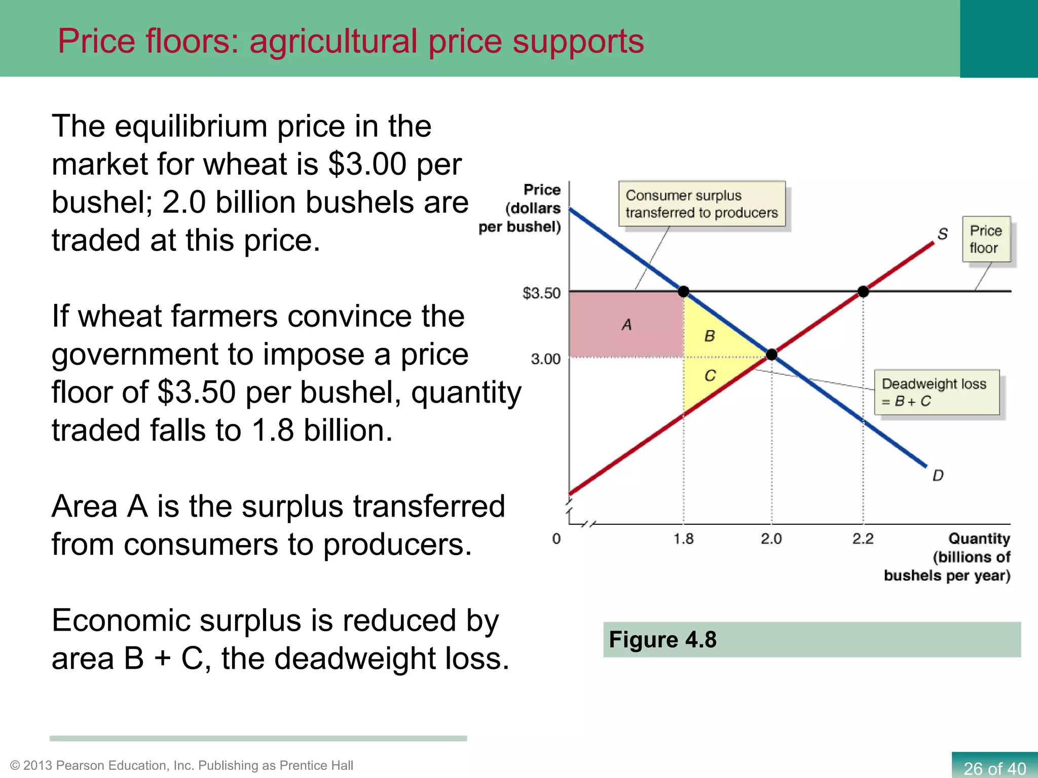
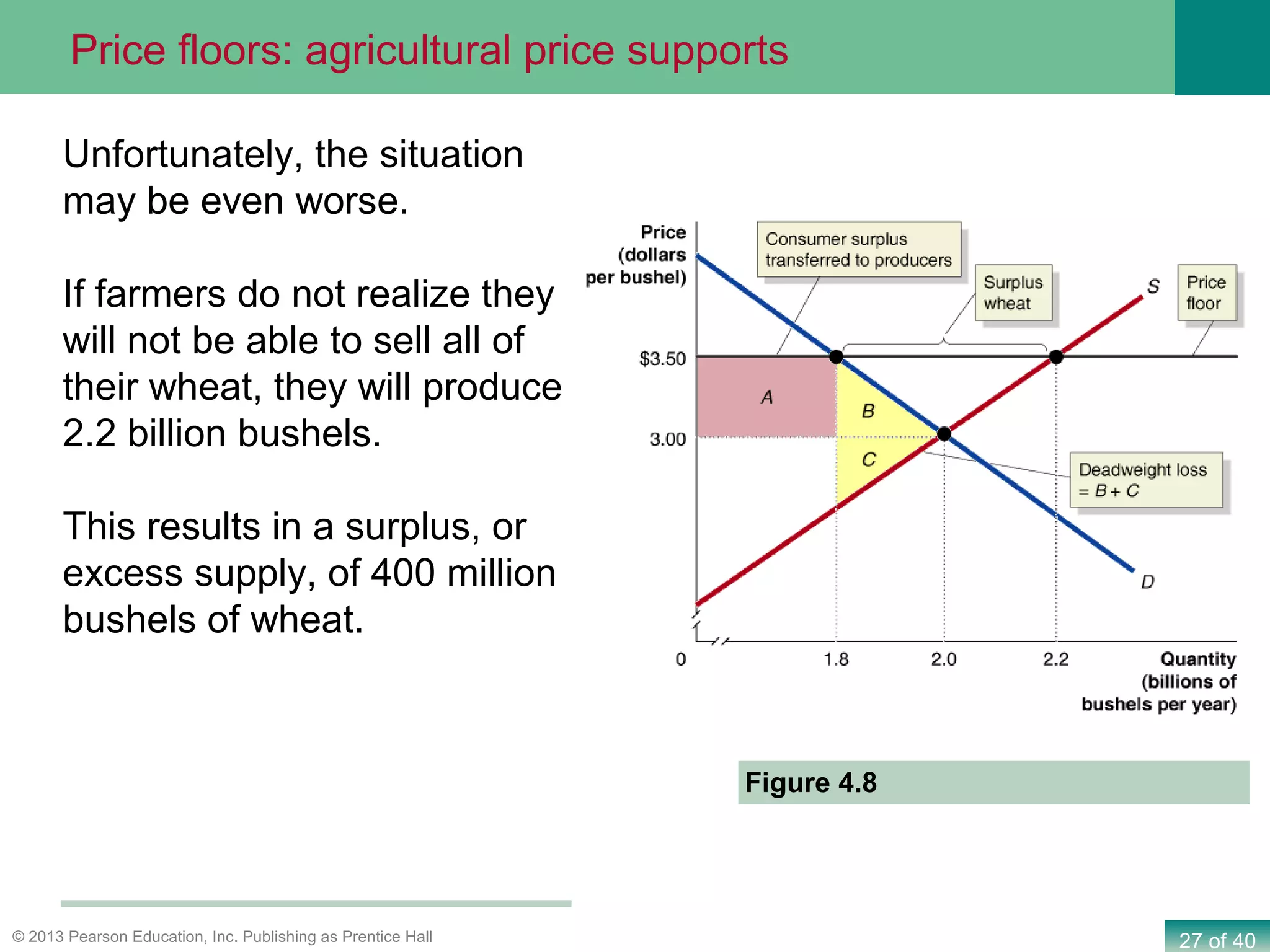
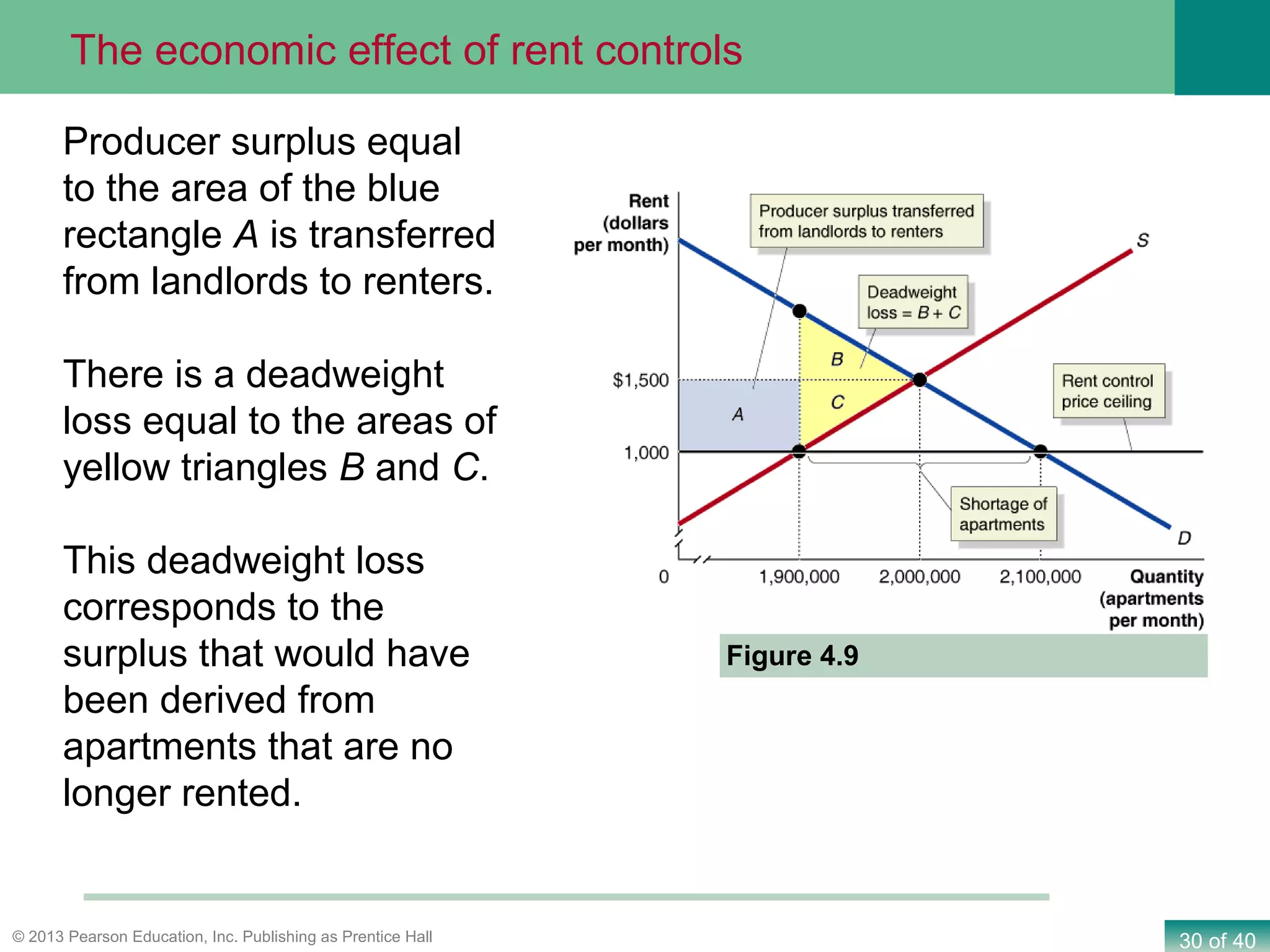
R. GLENN
HUBBAR
D
Economics
FOURTH EDITION
ANTHONY PATRICK
O’BRIE
N
2 of 40© 2013 Pearson Education, Inc. Publishing as Prentice Hall
Economic Efficiency, Government
Price Setting, and Taxes
CHAPTER
4
Chapter Outline and
Learning Objectives
4.1 Consumer Surplus and
Producer Surplus
4.2 The Efficiency of
Competitive Markets
4.3 Government Intervention
in the Market: Price Floors
and Price Ceilings
4.4 The Economic Impact of
Taxes
APPENDIX: Quantitative
Demand and Supply Analysis
3 of 40© 2013 Pearson Education, Inc. Publishing as Prentice Hall
Rent control puts a legal limit on the rent that landlords can
charge for an apartment.
Since rent-controlled rents are usually far below market rents, it
seems clear that this doesn’t make landlords better off.
Does it make tenants better off?
Should the Government Control Apartment Rents?
4 of 40© 2013 Pearson Education, Inc. Publishing as Prentice Hall
Distinguish between the concepts of consumer surplus and producer
surplus.
4.1 LEARNING OBJECTIVE
Consumer Surplus and Producer Surplus
5 of 40© 2013 Pearson Education, Inc. Publishing as Prentice Hall
Surplus (noun): Something that remains
above what is used or needed
Economists use the idea of “surplus” to refer to the benefit that
people derive from engaging in market transactions.
Consumer surplus refers to the dollar benefit consumers
receive from buying goods or services in a particular market.
Producer surplus refers to the dollar benefit firms receive from
buying goods or services in a particular market.
Consumer and producer surplus
6 of 40© 2013 Pearson Education, Inc. Publishing as Prentice Hall
Suppose four people
are each interested in
buying a cup of chai
tea.
We can characterize
them by the highest
price they are willing to
pay.
At prices above $6, no
chai tea will be sold.
At $6, one cup will be
sold, etc.
Figure 4.1
Deriving the demand curve for chai tea
7 of 40© 2013 Pearson Education, Inc. Publishing as Prentice Hall
How much benefit
do the potential tea
consumers derive
from this market?
That depends on
the price.
If the price is low,
many of the
consumers benefit.
If the price is high,
few (if any) of the
consumers benefit.
Figure 4.1
Thinking about the benefit derived by consumers
8 of 40© 2013 Pearson Education, Inc. Publishing as Prentice Hall
If the price of tea is $3.50 per
cup, Theresa, Tom, and Terri will
buy a cup.
Theresa was willing to pay $6.00;
a cup of chai tea is “worth” $6.00
to her. She got it for $3.50, so
she derives a net benefit of
$6.00 – $3.50 = $2.50.
Area A represents this net
benefit, and is known as
Theresa’s consumer surplus in
the chai tea market.
Figure 4.2
Consumer surplus at a price of $3.50
9 of 40© 2013 Pearson Education, Inc. Publishing as Prentice Hall
Tom and Terri also obtain
consumer surplus, equal to
$1.50 (area B) and $0.50 (area
C).
The sum of the areas of
rectangles A, B, and C is called
the consumer surplus in the
chai tea market.
This area can be described as
the area below the demand
curve, above the price that
consumers pay.
Figure 4.2
Consumer surplus at a price of $3.50
10 of 40© 2013 Pearson Education, Inc. Publishing as Prentice Hall
Figure 4.2
Consumer surplus at a price of $3.00
If the price falls to $3.00,
Theresa, Tom, and Terri each
gain an additional $0.50 of
consumer surplus.
Tim is indifferent between
buying the cup and not; his well-
being is the same either way.
The overall consumer surplus
remains the area below the
demand curve, above the (new)
price.
11 of 40© 2013 Pearson Education, Inc. Publishing as Prentice Hall
The market for chai tea
is larger than just our
four consumers.
With many consumers,
the market demand
curve looks like
“normal”: a straight line.
Consumer surplus in
this market is defined in
just the same way: the
area below the demand
curve, above price. The
graph shows consumer
surplus if price is $2.00.
Figure 4.3
Total consumer surplus in the market for chai tea
12 of 40© 2013 Pearson Education, Inc. Publishing as Prentice Hall
Having access to a broadband internet connection is beneficial
for consumers.
We can measure just how beneficial it is by estimating the
consumer surplus derived in the market.
What would we need to know in order to do this?
•The demand curve for broadband internet service
•The price of broadband internet service
The Consumer Surplus from
Broadband Internet Service
Making
the
Connection
13 of 40© 2013 Pearson Education, Inc. Publishing as Prentice Hall
In 2006, the average
price for broadband
internet service was $36
per month.
Economists Shane
Greenstein and Ryan
McDevitt estimated the
demand curve for
broadband internet
service, shown on the
right.
The Consumer Surplus from
Broadband Internet Service
Making
the
Connection
CS = Area of shaded triangle
= ½ (47 – 0) ($73.89 – $36)
= $890.4 million per month
14 of 40© 2013 Pearson Education, Inc. Publishing as Prentice Hall
Producer surplus in the chai tea latte market
Producer surplus can be thought of in much the same way as
consumer surplus.
It is the difference between the lowest price a firm would accept
for a good or service and the price it actually receives.
What is the lowest price a firm would accept for a good or
service?
The marginal cost of producing that good or service.
Marginal cost: the additional cost to a firm of producing one
more unit of a good or service.
15 of 40© 2013 Pearson Education, Inc. Publishing as Prentice Hall
Heavenly Tea is a
(very small) producer
of chai tea.
When the market price
of tea is $2.00,
Heavenly Tea receives
producer surplus of
$0.75 on the first cup
(the area of rectangle
A), $0.50 on the
second cup (rectangle
B), and $0.25 on the
third cup (rectangle C).
Figure 4.4a
Measuring producer surplus (single firm)
16 of 40© 2013 Pearson Education, Inc. Publishing as Prentice Hall
The total amount of
producer surplus tea
sellers receive from
selling chai tea can be
calculated by adding up
for the entire market the
producer surplus
received on each cup
sold.
Total producer surplus is
equal to the area above
the supply curve and
below the market price
of $2.00.
Figure 4.4b
Measuring producer surplus (entire market)
17 of 40© 2013 Pearson Education, Inc. Publishing as Prentice Hall
Consumer surplus measures the net benefit to consumers from
participating in a market rather than the total benefit.
Consumer surplus in a market is equal to the total benefit
received by consumers minus the total amount they must pay to
buy the good or service.
Similarly, producer surplus measures the net benefit received by
producers from participating in a market.
Producer surplus in a market is equal to the total amount firms
receive from consumers minus the cost of producing the good or
service.
What Consumer Surplus and Producer Surplus MeasureWhat do consumer and producer surplus measure?
18 of 40© 2013 Pearson Education, Inc. Publishing as Prentice Hall
Understand the concept of economic efficiency.
4.2 LEARNING OBJECTIVE
The Efficiency of Competitive Markets
19 of 40© 2013 Pearson Education, Inc. Publishing as Prentice Hall
We can think about efficiency in a market in two ways:
1.A market is efficient if all trades take place where the marginal
benefit exceeds the marginal cost, and no other trades take
place.
2.A market is efficient if it maximizes the sum of consumer and
producer surplus (i.e. the total net benefit to consumers and
firms), known as the economic surplus.
Marginal benefit: The additional benefit to a consumer from
consuming one more unit of a good or service.
Marginal cost: The additional cost to a firm of producing one
more unit of a good or service.
What Consumer Surplus and Producer Surplus MeasureHow much output is efficient?
20 of 40© 2013 Pearson Education, Inc. Publishing as Prentice Hall
• Every cup produced is sold at a price higher than its marginal cost.
• Every cup is bought at a price lower than its marginal benefit.
• There are no more additional cups that could be traded for which
the above two statements are true.
Only at a quantity of 15000 can all of these criteria be satisfied.
In the competitive
equilibrium, price
and quantity are
determined by
supply and demand.
The equilibrium
quantity is
economically
efficient:
Figure 4.5
The efficiency of competitive equilibrium
21 of 40© 2013 Pearson Education, Inc. Publishing as Prentice Hall
The figure shows the
economic surplus
(the sum of
consumer and
producer surplus) in
the market for chai
tea.
At the competitive
equilibrium quantity,
the economic surplus
is maximized. Figure 4.6
Our two concepts of economic efficiency are identical!
The efficiency of competitive equilibrium – surplus version
22 of 40© 2013 Pearson Education, Inc. Publishing as Prentice Hall
Figure 4.7
When the price of chai tea is $2.20 instead of $2.00, consumer
surplus declines from an amount equal to the sum of areas A, B,
and C to just area A.
Producer surplus increases from the sum of areas D and E to the
sum of areas B and D.
Economic surplus decreases by the sum of areas C and E.
Economic surplus, if the market is not in equilibrium
23 of 40© 2013 Pearson Education, Inc. Publishing as Prentice Hall
Figure 4.7
The reduction in economic surplus resulting from a market not
being in competitive equilibrium is known as deadweight loss.
Deadweight loss can be thought of as the amount of inefficiency
in a market. In competitive equilibrium, deadweight loss is zero.
Economic surplus, if the market is not in equilibrium
24 of 40© 2013 Pearson Education, Inc. Publishing as Prentice Hall
Explain the economic effect of government-imposed price floors and price
ceilings.
4.3 LEARNING OBJECTIVE
Government Intervention in the Market:
Price Floors and Price Ceilings
25 of 40© 2013 Pearson Education, Inc. Publishing as Prentice Hall
One option a government has for affecting a market is the
imposition of a price ceiling or a price floor.
Price ceiling: A legally determined maximum price that
sellers can charge.
Price floor: A legally determined minimum price that
sellers may receive.
Price ceilings and floors in the USA are uncommon, but include:
•Minimum wages
•Rent controls
•Agricultural price controls
What Consumer Surplus and Producer Surplus MeasurePrice ceilings and floors
26 of 40© 2013 Pearson Education, Inc. Publishing as Prentice Hall
Figure 4.8
The equilibrium price in the
market for wheat is $3.00 per
bushel; 2.0 billion bushels are
traded at this price.
If wheat farmers convince the
government to impose a price
floor of $3.50 per bushel, quantity
traded falls to 1.8 billion.
Area A is the surplus transferred
from consumers to producers.
Economic surplus is reduced by
area B + C, the deadweight loss.
Price floors: agricultural price supports
27 of 40© 2013 Pearson Education, Inc. Publishing as Prentice Hall
Figure 4.8
Unfortunately, the situation
may be even worse.
If farmers do not realize they
will not be able to sell all of
their wheat, they will produce
2.2 billion bushels.
This results in a surplus, or
excess supply, of 400 million
bushels of wheat.
Price floors: agricultural price supports
28 of 40© 2013 Pearson Education, Inc. Publishing as Prentice Hall
Price Floors in Labor Markets: The Debate
over Minimum Wage Policy
Making
the
Connection
Supporters of the
minimum wage see it
as a way of raising
the incomes of low-
skilled workers.
Opponents argue
that it results in fewer
jobs and imposes
large costs on small
businesses.
Assuming the minimum wage does decrease employment, it
must result in a deadweight loss for society.
29 of 40© 2013 Pearson Education, Inc. Publishing as Prentice Hall
Figure 4.9
Without rent control, the
equilibrium rent is $1,500 per
month.
At that price, 2,000,000
apartments would be rented.
If the government imposes a
rent ceiling of $1,000, the
quantity of apartments supplied
falls to 1,900,000,
and the quantity of apartments
demanded increases to
2,100,000,
resulting in a shortage of
200,000 apartments.
Price ceilings: rent control
30 of 40© 2013 Pearson Education, Inc. Publishing as Prentice Hall
Producer surplus equal
to the area of the blue
rectangle A is transferred
from landlords to renters.
There is a deadweight
loss equal to the areas of
yellow triangles B and C.
This deadweight loss
corresponds to the
surplus that would have
been derived from
apartments that are no
longer rented.
The economic effect of rent controls
Figure 4.9
31 of 40© 2013 Pearson Education, Inc. Publishing as Prentice Hall
The shortage of apartments may lead to a black market – a
market in which buying and selling take place at prices that
violate government price regulations.
The existence of a black market may alleviate some of the
deadweight loss by allowing additional apartments to be rented;
but buyers and sellers lose valuable legal protections.
Additionally, landlords may not have strong incentives to
maintain rent-controlled apartments, so the apartments may fall
into disrepair.
Over time, landlords may even abandon some apartment
buildings.
What Consumer Surplus and Producer Surplus MeasureUnintended effects of rent controls
32 of 40© 2013 Pearson Education, Inc. Publishing as Prentice Hall
It is clear that when a government imposes price controls,
• Some people are made better off
• Some people are made worse off
• The economy generally suffers, as deadweight loss will
generally occur
Economists seldom recommend price controls, with the possible
exception of minimum wage laws. Why minimum wage laws?
• Price controls might be justified if there are strong equity
effects to override the efficiency loss.
• The people benefitting from minimum wage laws are generally
poor.
The results of government price controls
33 of 40© 2013 Pearson Education, Inc. Publishing as Prentice Hall
Analyze the economic impact of taxes.
4.4 LEARNING OBJECTIVE
The Economic Impact of Taxes
34 of 40© 2013 Pearson Education, Inc. Publishing as Prentice Hall
Taxes are the most important method by which governments
fund their activities.
We will concentrate on per-unit taxes: taxes assessed as a
particular dollar amount on the sale of a good or service, as
opposed to a percentage tax.
Example: The US Federal government imposes a 18.4 cents per
gallon tax on gasoline sales, as of 2012.
source: http://www.gaspricewatch.com/web_gas_taxes.php
What Consumer Surplus and Producer Surplus MeasureTaxes
35 of 40© 2013 Pearson Education, Inc. Publishing as Prentice Hall
Without the tax, market
equilibrium occurs at
point A.
The equilibrium price of
cigarettes is $4.00 per
pack, and 4 billion
packs of cigarettes are
sold per year.
A $1.00-per-pack tax on
cigarettes will cause the
supply curve for
cigarettes to shift up by
$1.00, from S1 to S2.
The effect of a tax on cigarettes
The new equilibrium occurs at point B.
The price of cigarettes will increase by $0.90, to $4.90 per pack, and
the quantity sold will fall to 3.7 billion packs.
Figure 4.10
36 of 40© 2013 Pearson Education, Inc. Publishing as Prentice Hall
The supply curve shifted
up by $1.00, the amount
of the tax.
If firms were willing to
sell 4 billion packs at a
price of $4.00 before the
tax, the price needs to
be exactly $1.00 higher
in order to convince
them to still sell 4 billion
packs.
This is because firms’
costs effectively
increased by $1.00 per
unit.
What just happened with the supply curve?
Figure 4.10
37 of 40© 2013 Pearson Education, Inc. Publishing as Prentice Hall
Cigarette tax revenue and deadweight loss
Figure 4.10The tax increases the
price paid by consumers
to $4.90 per pack.
Producers receive a
price of $4.90 per pack
(point B), but after
paying the $1.00 tax,
they are left with $3.90
(point C).
The government will receive tax revenue equal to the green shaded
box.
Some consumer surplus and some producer surplus will become
tax revenue for the government, and some will become deadweight
loss, shown by the yellow-shaded area.
38 of 40© 2013 Pearson Education, Inc. Publishing as Prentice Hall
Figure 4.11
With no tax on gasoline,
the price would be $3.00
per gallon, and 144 billion
gallons of gasoline would
be sold each year.
A 10-cents-per-gallon
excise tax shifts up the
supply curve from S1 to S2.
The price consumers pay
rises from $3.00 to $3.08.
The price sellers receive
falls from $3.00 to $2.98.
Determining tax incidence on a demand and supply graph
Therefore, consumers pay 8 cents of the 10-cents-per-gallon tax
on gasoline, and sellers pay 2 cents.
39 of 40© 2013 Pearson Education, Inc. Publishing as Prentice Hall
In the market for gasoline, the buyers effectively paid 80% of the
10-cents-per-gallon tax, and sellers paid 20%.
This is referred to as the tax incidence: the actual division of the
burden of a tax between buyers and sellers in a market.
What determines this tax incidence? As we will see on the next
slide, the answer is not “whoever has the legal obligation to pay
the tax”…
What Consumer Surplus and Producer Surplus MeasureTax incidence: who actually pays a tax?
40 of 40© 2013 Pearson Education, Inc. Publishing as Prentice Hall
This is the same result we saw when producers were responsible
for paying the tax!
Figure 4.12
With no tax on
gasoline, the demand
curve is D1.
If a 10-cents-per-
gallon tax imposed on
consumers, the
demand curve shifts
down by the amount of
the tax, from D1 to D2.
In the new equilibrium,
consumers pay a price
of $3.08 per gallon,
including the tax.
Producers receive
$2.98 per gallon.
What if the buyers were legally obligated to pay the tax?
41 of 40© 2013 Pearson Education, Inc. Publishing as Prentice Hall
The incidence of the tax is determined by the relative slopes of
the demand and supply curves.
A steep demand curve means that buyers do not change how
much they buy when the price changes; this results in them
taking on much of the burden of the tax.
If the demand curve were shallower, buyers would change how
much they bought a lot in response to a price change. Then they
could not be forced to accept as much of the burden of the tax.
Similar analysis applies for sellers.
What Consumer Surplus and Producer Surplus MeasureWhat determines the tax incidence?
42 of 40© 2013 Pearson Education, Inc. Publishing as Prentice Hall
Is the Burden of the Social Security Tax Really
Shared Equally between Workers and Firms?
Making
the
Connection
The Federal Insurance Contributions Act (FICA) tax is 15.3% of
wages, and funds Social Security and Medicare. By law,
employers pay half (7.65%), as do workers.
Who really ends up with most of the burden of this tax?
The answer depends on who is less sensitive to changes in
wages: employers (buyers of labor) or workers (sellers of labor).
It turns out that workers are relatively insensitive to their wages;
that is, they don’t change their hours-of-work decision much
when their wages change.
So workers end up with most of the burden of this tax.
43 of 40© 2013 Pearson Education, Inc. Publishing as Prentice Hall
Is the Burden of the Social Security Tax Really
Shared Equally between Workers and Firms?
Making
the
Connection
The panels illustrate an imaginary $1.00 per hour Social Security tax.
Whether firms or workers have the legal obligation to pay the tax,
workers end up with most of the tax burden.
44 of 40© 2013 Pearson Education, Inc. Publishing as Prentice Hall
Scarcity and shortage both have technical meanings. There is no
shortage of most scarce goods.
Price ceilings are only effective if they are placed below the
equilibrium price. Similarly, price floors are effective only when
above the equilibrium price.
When showing a tax, if sellers are legally obligated to pay the
tax, move the supply curve up by the amount of the tax; if buyers
are obligated to pay the tax, move the demand curve down by
the amount of the tax.
The legal obligation to pay a tax is not the same as the tax
burden.
Common misconceptions to avoid
45 of 40© 2013 Pearson Education, Inc. Publishing as Prentice Hall
Quantitative Demand and Supply AnalysisAppendix
Use quantitative demand and supply analysis.
LEARNING OBJECTIVE
Demand and Supply Equations
Suppose that the demand for apartments in New York City is
QD
= 3,000,000 − 1,000P
and the supply of apartments is
QS
= −450,000 + 1,300P
In equilibrium, we know QD
= QS
(This is known as the equilibrium condition.)
We use this to find the equilibrium rent and quantity:
3,000,000 − 1,000P = −450,000 + 1,300P
3,450,000 = 2300P
P= 1500
46 of 40© 2013 Pearson Education, Inc. Publishing as Prentice Hall
In order to graph the demand and supply curves, calculate the y-
intercepts by setting QD
and QS
equal to zero and solving for
price:
QD
= 0= 3,000,000 – (1000)P
1000P= 3,000,000
P= 3000
and
QS
= 0 = –450,000 + (1300)P
–(1300)P = –450,000
P= 346.15
Find the equilibrium quantity of apartments rented:
QD
= 3,000,000 – (1000)(1500)
= 1,500,000
QS
= – 450,000 + (1300)(1500)
= 1,500,000
Quantitative Demand and Supply AnalysisAppendix
47 of 40© 2013 Pearson Education, Inc. Publishing as Prentice Hall
Figure 4A.1
Graphing Supply and Demand
EquationsAll of the items calculated
on the previous slides are
elements of the demand
and supply graph:
•y-intercept for supply
•y-intercept for demand
•Equilibrium price
•Equilibrium quantity
Quantitative Demand and Supply AnalysisAppendix
48 of 40© 2013 Pearson Education, Inc. Publishing as Prentice Hall
Now we can calculate
estimated consumer and
producer surplus, using the
triangle area formula:
Area = ½ (base)(height)
CS = ½(1.5)($3000-$1500)
= $1125 million
PS = ½(1.5)($1500-$346)
= $865.5 million
Quantitative Demand and Supply AnalysisAppendix
Figure 4A.1
Graphing Supply and Demand
Equations
49 of 40© 2013 Pearson Education, Inc. Publishing as Prentice Hall
Suppose the city imposes a rent ceiling of $1,000 per month.
Calculate the quantity of apartments that will actually be rented:
Qs
= –450,000 + 1300P
= –450,000 + (1300)(1000)
= 850,000
Find the price on the demand curve when the quantity of
apartments is 850,000:
850000 = 3,000,000 – 1000P
–2,150,000 = –1000P
P = (–2,150,000)/(–1000)
= $2150
Quantitative Demand and Supply AnalysisAppendix
50 of 40© 2013 Pearson Education, Inc. Publishing as Prentice Hall
Figure 4A.2
Calculating the Economic Effect of Rent
Controls
Once we have estimated
equations for the demand
and supply of rental housing,
a diagram can guide our
numeric estimates of the
economic effects of rent
control.
Our figures from the previous
slide can now be inserted.
Triangles B+C represent
deadweight loss:
$373.75 million
Quantitative Demand and Supply AnalysisAppendix
51 of 40© 2013 Pearson Education, Inc. Publishing as Prentice Hall
Figure 4A.2
Calculating the Economic Effect of Rent
Controls
Consumer surplus falls by the
area of the yellow triangle B
and increases by the area of
the blue rectangle A.
The difference between the
values of these two areas is
$213.75 million.
Producer surplus falls by the
area of the blue rectangle A
plus the area of the yellow
triangle C.
The value of these two areas
is $587.5 million.
Quantitative Demand and Supply AnalysisAppendix
The remaining producer surplus is equal to the area of triangle
D, or $278 million.
52 of 40© 2013 Pearson Education, Inc. Publishing as Prentice Hall
Consumer Surplus Producer Surplus Deadweight Loss
Competitive
Equilibrium
Rent
Control
Competitive
Equilibrium
Rent
Control
Competitive
Equilibrium
Rent
Control
$1,125 $1,338.75 $865.50 $278 $0 $373.75
The following table summarizes the results of the analysis (the
values are in millions of dollars):
Quantitative Demand and Supply AnalysisAppendix

Ge273.u3.pp2

  • 1.
  • 2.
    2 of 40©2013 Pearson Education, Inc. Publishing as Prentice Hall Economic Efficiency, Government Price Setting, and Taxes CHAPTER 4 Chapter Outline and Learning Objectives 4.1 Consumer Surplus and Producer Surplus 4.2 The Efficiency of Competitive Markets 4.3 Government Intervention in the Market: Price Floors and Price Ceilings 4.4 The Economic Impact of Taxes APPENDIX: Quantitative Demand and Supply Analysis
  • 3.
    3 of 40©2013 Pearson Education, Inc. Publishing as Prentice Hall Rent control puts a legal limit on the rent that landlords can charge for an apartment. Since rent-controlled rents are usually far below market rents, it seems clear that this doesn’t make landlords better off. Does it make tenants better off? Should the Government Control Apartment Rents?
  • 4.
    4 of 40©2013 Pearson Education, Inc. Publishing as Prentice Hall Distinguish between the concepts of consumer surplus and producer surplus. 4.1 LEARNING OBJECTIVE Consumer Surplus and Producer Surplus
  • 5.
    5 of 40©2013 Pearson Education, Inc. Publishing as Prentice Hall Surplus (noun): Something that remains above what is used or needed Economists use the idea of “surplus” to refer to the benefit that people derive from engaging in market transactions. Consumer surplus refers to the dollar benefit consumers receive from buying goods or services in a particular market. Producer surplus refers to the dollar benefit firms receive from buying goods or services in a particular market. Consumer and producer surplus
  • 6.
    6 of 40©2013 Pearson Education, Inc. Publishing as Prentice Hall Suppose four people are each interested in buying a cup of chai tea. We can characterize them by the highest price they are willing to pay. At prices above $6, no chai tea will be sold. At $6, one cup will be sold, etc. Figure 4.1 Deriving the demand curve for chai tea
  • 7.
    7 of 40©2013 Pearson Education, Inc. Publishing as Prentice Hall How much benefit do the potential tea consumers derive from this market? That depends on the price. If the price is low, many of the consumers benefit. If the price is high, few (if any) of the consumers benefit. Figure 4.1 Thinking about the benefit derived by consumers
  • 8.
    8 of 40©2013 Pearson Education, Inc. Publishing as Prentice Hall If the price of tea is $3.50 per cup, Theresa, Tom, and Terri will buy a cup. Theresa was willing to pay $6.00; a cup of chai tea is “worth” $6.00 to her. She got it for $3.50, so she derives a net benefit of $6.00 – $3.50 = $2.50. Area A represents this net benefit, and is known as Theresa’s consumer surplus in the chai tea market. Figure 4.2 Consumer surplus at a price of $3.50
  • 9.
    9 of 40©2013 Pearson Education, Inc. Publishing as Prentice Hall Tom and Terri also obtain consumer surplus, equal to $1.50 (area B) and $0.50 (area C). The sum of the areas of rectangles A, B, and C is called the consumer surplus in the chai tea market. This area can be described as the area below the demand curve, above the price that consumers pay. Figure 4.2 Consumer surplus at a price of $3.50
  • 10.
    10 of 40©2013 Pearson Education, Inc. Publishing as Prentice Hall Figure 4.2 Consumer surplus at a price of $3.00 If the price falls to $3.00, Theresa, Tom, and Terri each gain an additional $0.50 of consumer surplus. Tim is indifferent between buying the cup and not; his well- being is the same either way. The overall consumer surplus remains the area below the demand curve, above the (new) price.
  • 11.
    11 of 40©2013 Pearson Education, Inc. Publishing as Prentice Hall The market for chai tea is larger than just our four consumers. With many consumers, the market demand curve looks like “normal”: a straight line. Consumer surplus in this market is defined in just the same way: the area below the demand curve, above price. The graph shows consumer surplus if price is $2.00. Figure 4.3 Total consumer surplus in the market for chai tea
  • 12.
    12 of 40©2013 Pearson Education, Inc. Publishing as Prentice Hall Having access to a broadband internet connection is beneficial for consumers. We can measure just how beneficial it is by estimating the consumer surplus derived in the market. What would we need to know in order to do this? •The demand curve for broadband internet service •The price of broadband internet service The Consumer Surplus from Broadband Internet Service Making the Connection
  • 13.
    13 of 40©2013 Pearson Education, Inc. Publishing as Prentice Hall In 2006, the average price for broadband internet service was $36 per month. Economists Shane Greenstein and Ryan McDevitt estimated the demand curve for broadband internet service, shown on the right. The Consumer Surplus from Broadband Internet Service Making the Connection CS = Area of shaded triangle = ½ (47 – 0) ($73.89 – $36) = $890.4 million per month
  • 14.
    14 of 40©2013 Pearson Education, Inc. Publishing as Prentice Hall Producer surplus in the chai tea latte market Producer surplus can be thought of in much the same way as consumer surplus. It is the difference between the lowest price a firm would accept for a good or service and the price it actually receives. What is the lowest price a firm would accept for a good or service? The marginal cost of producing that good or service. Marginal cost: the additional cost to a firm of producing one more unit of a good or service.
  • 15.
    15 of 40©2013 Pearson Education, Inc. Publishing as Prentice Hall Heavenly Tea is a (very small) producer of chai tea. When the market price of tea is $2.00, Heavenly Tea receives producer surplus of $0.75 on the first cup (the area of rectangle A), $0.50 on the second cup (rectangle B), and $0.25 on the third cup (rectangle C). Figure 4.4a Measuring producer surplus (single firm)
  • 16.
    16 of 40©2013 Pearson Education, Inc. Publishing as Prentice Hall The total amount of producer surplus tea sellers receive from selling chai tea can be calculated by adding up for the entire market the producer surplus received on each cup sold. Total producer surplus is equal to the area above the supply curve and below the market price of $2.00. Figure 4.4b Measuring producer surplus (entire market)
  • 17.
    17 of 40©2013 Pearson Education, Inc. Publishing as Prentice Hall Consumer surplus measures the net benefit to consumers from participating in a market rather than the total benefit. Consumer surplus in a market is equal to the total benefit received by consumers minus the total amount they must pay to buy the good or service. Similarly, producer surplus measures the net benefit received by producers from participating in a market. Producer surplus in a market is equal to the total amount firms receive from consumers minus the cost of producing the good or service. What Consumer Surplus and Producer Surplus MeasureWhat do consumer and producer surplus measure?
  • 18.
    18 of 40©2013 Pearson Education, Inc. Publishing as Prentice Hall Understand the concept of economic efficiency. 4.2 LEARNING OBJECTIVE The Efficiency of Competitive Markets
  • 19.
    19 of 40©2013 Pearson Education, Inc. Publishing as Prentice Hall We can think about efficiency in a market in two ways: 1.A market is efficient if all trades take place where the marginal benefit exceeds the marginal cost, and no other trades take place. 2.A market is efficient if it maximizes the sum of consumer and producer surplus (i.e. the total net benefit to consumers and firms), known as the economic surplus. Marginal benefit: The additional benefit to a consumer from consuming one more unit of a good or service. Marginal cost: The additional cost to a firm of producing one more unit of a good or service. What Consumer Surplus and Producer Surplus MeasureHow much output is efficient?
  • 20.
    20 of 40©2013 Pearson Education, Inc. Publishing as Prentice Hall • Every cup produced is sold at a price higher than its marginal cost. • Every cup is bought at a price lower than its marginal benefit. • There are no more additional cups that could be traded for which the above two statements are true. Only at a quantity of 15000 can all of these criteria be satisfied. In the competitive equilibrium, price and quantity are determined by supply and demand. The equilibrium quantity is economically efficient: Figure 4.5 The efficiency of competitive equilibrium
  • 21.
    21 of 40©2013 Pearson Education, Inc. Publishing as Prentice Hall The figure shows the economic surplus (the sum of consumer and producer surplus) in the market for chai tea. At the competitive equilibrium quantity, the economic surplus is maximized. Figure 4.6 Our two concepts of economic efficiency are identical! The efficiency of competitive equilibrium – surplus version
  • 22.
    22 of 40©2013 Pearson Education, Inc. Publishing as Prentice Hall Figure 4.7 When the price of chai tea is $2.20 instead of $2.00, consumer surplus declines from an amount equal to the sum of areas A, B, and C to just area A. Producer surplus increases from the sum of areas D and E to the sum of areas B and D. Economic surplus decreases by the sum of areas C and E. Economic surplus, if the market is not in equilibrium
  • 23.
    23 of 40©2013 Pearson Education, Inc. Publishing as Prentice Hall Figure 4.7 The reduction in economic surplus resulting from a market not being in competitive equilibrium is known as deadweight loss. Deadweight loss can be thought of as the amount of inefficiency in a market. In competitive equilibrium, deadweight loss is zero. Economic surplus, if the market is not in equilibrium
  • 24.
    24 of 40©2013 Pearson Education, Inc. Publishing as Prentice Hall Explain the economic effect of government-imposed price floors and price ceilings. 4.3 LEARNING OBJECTIVE Government Intervention in the Market: Price Floors and Price Ceilings
  • 25.
    25 of 40©2013 Pearson Education, Inc. Publishing as Prentice Hall One option a government has for affecting a market is the imposition of a price ceiling or a price floor. Price ceiling: A legally determined maximum price that sellers can charge. Price floor: A legally determined minimum price that sellers may receive. Price ceilings and floors in the USA are uncommon, but include: •Minimum wages •Rent controls •Agricultural price controls What Consumer Surplus and Producer Surplus MeasurePrice ceilings and floors
  • 26.
    26 of 40©2013 Pearson Education, Inc. Publishing as Prentice Hall Figure 4.8 The equilibrium price in the market for wheat is $3.00 per bushel; 2.0 billion bushels are traded at this price. If wheat farmers convince the government to impose a price floor of $3.50 per bushel, quantity traded falls to 1.8 billion. Area A is the surplus transferred from consumers to producers. Economic surplus is reduced by area B + C, the deadweight loss. Price floors: agricultural price supports
  • 27.
    27 of 40©2013 Pearson Education, Inc. Publishing as Prentice Hall Figure 4.8 Unfortunately, the situation may be even worse. If farmers do not realize they will not be able to sell all of their wheat, they will produce 2.2 billion bushels. This results in a surplus, or excess supply, of 400 million bushels of wheat. Price floors: agricultural price supports
  • 28.
    28 of 40©2013 Pearson Education, Inc. Publishing as Prentice Hall Price Floors in Labor Markets: The Debate over Minimum Wage Policy Making the Connection Supporters of the minimum wage see it as a way of raising the incomes of low- skilled workers. Opponents argue that it results in fewer jobs and imposes large costs on small businesses. Assuming the minimum wage does decrease employment, it must result in a deadweight loss for society.
  • 29.
    29 of 40©2013 Pearson Education, Inc. Publishing as Prentice Hall Figure 4.9 Without rent control, the equilibrium rent is $1,500 per month. At that price, 2,000,000 apartments would be rented. If the government imposes a rent ceiling of $1,000, the quantity of apartments supplied falls to 1,900,000, and the quantity of apartments demanded increases to 2,100,000, resulting in a shortage of 200,000 apartments. Price ceilings: rent control
  • 30.
    30 of 40©2013 Pearson Education, Inc. Publishing as Prentice Hall Producer surplus equal to the area of the blue rectangle A is transferred from landlords to renters. There is a deadweight loss equal to the areas of yellow triangles B and C. This deadweight loss corresponds to the surplus that would have been derived from apartments that are no longer rented. The economic effect of rent controls Figure 4.9
  • 31.
    31 of 40©2013 Pearson Education, Inc. Publishing as Prentice Hall The shortage of apartments may lead to a black market – a market in which buying and selling take place at prices that violate government price regulations. The existence of a black market may alleviate some of the deadweight loss by allowing additional apartments to be rented; but buyers and sellers lose valuable legal protections. Additionally, landlords may not have strong incentives to maintain rent-controlled apartments, so the apartments may fall into disrepair. Over time, landlords may even abandon some apartment buildings. What Consumer Surplus and Producer Surplus MeasureUnintended effects of rent controls
  • 32.
    32 of 40©2013 Pearson Education, Inc. Publishing as Prentice Hall It is clear that when a government imposes price controls, • Some people are made better off • Some people are made worse off • The economy generally suffers, as deadweight loss will generally occur Economists seldom recommend price controls, with the possible exception of minimum wage laws. Why minimum wage laws? • Price controls might be justified if there are strong equity effects to override the efficiency loss. • The people benefitting from minimum wage laws are generally poor. The results of government price controls
  • 33.
    33 of 40©2013 Pearson Education, Inc. Publishing as Prentice Hall Analyze the economic impact of taxes. 4.4 LEARNING OBJECTIVE The Economic Impact of Taxes
  • 34.
    34 of 40©2013 Pearson Education, Inc. Publishing as Prentice Hall Taxes are the most important method by which governments fund their activities. We will concentrate on per-unit taxes: taxes assessed as a particular dollar amount on the sale of a good or service, as opposed to a percentage tax. Example: The US Federal government imposes a 18.4 cents per gallon tax on gasoline sales, as of 2012. source: http://www.gaspricewatch.com/web_gas_taxes.php What Consumer Surplus and Producer Surplus MeasureTaxes
  • 35.
    35 of 40©2013 Pearson Education, Inc. Publishing as Prentice Hall Without the tax, market equilibrium occurs at point A. The equilibrium price of cigarettes is $4.00 per pack, and 4 billion packs of cigarettes are sold per year. A $1.00-per-pack tax on cigarettes will cause the supply curve for cigarettes to shift up by $1.00, from S1 to S2. The effect of a tax on cigarettes The new equilibrium occurs at point B. The price of cigarettes will increase by $0.90, to $4.90 per pack, and the quantity sold will fall to 3.7 billion packs. Figure 4.10
  • 36.
    36 of 40©2013 Pearson Education, Inc. Publishing as Prentice Hall The supply curve shifted up by $1.00, the amount of the tax. If firms were willing to sell 4 billion packs at a price of $4.00 before the tax, the price needs to be exactly $1.00 higher in order to convince them to still sell 4 billion packs. This is because firms’ costs effectively increased by $1.00 per unit. What just happened with the supply curve? Figure 4.10
  • 37.
    37 of 40©2013 Pearson Education, Inc. Publishing as Prentice Hall Cigarette tax revenue and deadweight loss Figure 4.10The tax increases the price paid by consumers to $4.90 per pack. Producers receive a price of $4.90 per pack (point B), but after paying the $1.00 tax, they are left with $3.90 (point C). The government will receive tax revenue equal to the green shaded box. Some consumer surplus and some producer surplus will become tax revenue for the government, and some will become deadweight loss, shown by the yellow-shaded area.
  • 38.
    38 of 40©2013 Pearson Education, Inc. Publishing as Prentice Hall Figure 4.11 With no tax on gasoline, the price would be $3.00 per gallon, and 144 billion gallons of gasoline would be sold each year. A 10-cents-per-gallon excise tax shifts up the supply curve from S1 to S2. The price consumers pay rises from $3.00 to $3.08. The price sellers receive falls from $3.00 to $2.98. Determining tax incidence on a demand and supply graph Therefore, consumers pay 8 cents of the 10-cents-per-gallon tax on gasoline, and sellers pay 2 cents.
  • 39.
    39 of 40©2013 Pearson Education, Inc. Publishing as Prentice Hall In the market for gasoline, the buyers effectively paid 80% of the 10-cents-per-gallon tax, and sellers paid 20%. This is referred to as the tax incidence: the actual division of the burden of a tax between buyers and sellers in a market. What determines this tax incidence? As we will see on the next slide, the answer is not “whoever has the legal obligation to pay the tax”… What Consumer Surplus and Producer Surplus MeasureTax incidence: who actually pays a tax?
  • 40.
    40 of 40©2013 Pearson Education, Inc. Publishing as Prentice Hall This is the same result we saw when producers were responsible for paying the tax! Figure 4.12 With no tax on gasoline, the demand curve is D1. If a 10-cents-per- gallon tax imposed on consumers, the demand curve shifts down by the amount of the tax, from D1 to D2. In the new equilibrium, consumers pay a price of $3.08 per gallon, including the tax. Producers receive $2.98 per gallon. What if the buyers were legally obligated to pay the tax?
  • 41.
    41 of 40©2013 Pearson Education, Inc. Publishing as Prentice Hall The incidence of the tax is determined by the relative slopes of the demand and supply curves. A steep demand curve means that buyers do not change how much they buy when the price changes; this results in them taking on much of the burden of the tax. If the demand curve were shallower, buyers would change how much they bought a lot in response to a price change. Then they could not be forced to accept as much of the burden of the tax. Similar analysis applies for sellers. What Consumer Surplus and Producer Surplus MeasureWhat determines the tax incidence?
  • 42.
    42 of 40©2013 Pearson Education, Inc. Publishing as Prentice Hall Is the Burden of the Social Security Tax Really Shared Equally between Workers and Firms? Making the Connection The Federal Insurance Contributions Act (FICA) tax is 15.3% of wages, and funds Social Security and Medicare. By law, employers pay half (7.65%), as do workers. Who really ends up with most of the burden of this tax? The answer depends on who is less sensitive to changes in wages: employers (buyers of labor) or workers (sellers of labor). It turns out that workers are relatively insensitive to their wages; that is, they don’t change their hours-of-work decision much when their wages change. So workers end up with most of the burden of this tax.
  • 43.
    43 of 40©2013 Pearson Education, Inc. Publishing as Prentice Hall Is the Burden of the Social Security Tax Really Shared Equally between Workers and Firms? Making the Connection The panels illustrate an imaginary $1.00 per hour Social Security tax. Whether firms or workers have the legal obligation to pay the tax, workers end up with most of the tax burden.
  • 44.
    44 of 40©2013 Pearson Education, Inc. Publishing as Prentice Hall Scarcity and shortage both have technical meanings. There is no shortage of most scarce goods. Price ceilings are only effective if they are placed below the equilibrium price. Similarly, price floors are effective only when above the equilibrium price. When showing a tax, if sellers are legally obligated to pay the tax, move the supply curve up by the amount of the tax; if buyers are obligated to pay the tax, move the demand curve down by the amount of the tax. The legal obligation to pay a tax is not the same as the tax burden. Common misconceptions to avoid
  • 45.
    45 of 40©2013 Pearson Education, Inc. Publishing as Prentice Hall Quantitative Demand and Supply AnalysisAppendix Use quantitative demand and supply analysis. LEARNING OBJECTIVE Demand and Supply Equations Suppose that the demand for apartments in New York City is QD = 3,000,000 − 1,000P and the supply of apartments is QS = −450,000 + 1,300P In equilibrium, we know QD = QS (This is known as the equilibrium condition.) We use this to find the equilibrium rent and quantity: 3,000,000 − 1,000P = −450,000 + 1,300P 3,450,000 = 2300P P= 1500
  • 46.
    46 of 40©2013 Pearson Education, Inc. Publishing as Prentice Hall In order to graph the demand and supply curves, calculate the y- intercepts by setting QD and QS equal to zero and solving for price: QD = 0= 3,000,000 – (1000)P 1000P= 3,000,000 P= 3000 and QS = 0 = –450,000 + (1300)P –(1300)P = –450,000 P= 346.15 Find the equilibrium quantity of apartments rented: QD = 3,000,000 – (1000)(1500) = 1,500,000 QS = – 450,000 + (1300)(1500) = 1,500,000 Quantitative Demand and Supply AnalysisAppendix
  • 47.
    47 of 40©2013 Pearson Education, Inc. Publishing as Prentice Hall Figure 4A.1 Graphing Supply and Demand EquationsAll of the items calculated on the previous slides are elements of the demand and supply graph: •y-intercept for supply •y-intercept for demand •Equilibrium price •Equilibrium quantity Quantitative Demand and Supply AnalysisAppendix
  • 48.
    48 of 40©2013 Pearson Education, Inc. Publishing as Prentice Hall Now we can calculate estimated consumer and producer surplus, using the triangle area formula: Area = ½ (base)(height) CS = ½(1.5)($3000-$1500) = $1125 million PS = ½(1.5)($1500-$346) = $865.5 million Quantitative Demand and Supply AnalysisAppendix Figure 4A.1 Graphing Supply and Demand Equations
  • 49.
    49 of 40©2013 Pearson Education, Inc. Publishing as Prentice Hall Suppose the city imposes a rent ceiling of $1,000 per month. Calculate the quantity of apartments that will actually be rented: Qs = –450,000 + 1300P = –450,000 + (1300)(1000) = 850,000 Find the price on the demand curve when the quantity of apartments is 850,000: 850000 = 3,000,000 – 1000P –2,150,000 = –1000P P = (–2,150,000)/(–1000) = $2150 Quantitative Demand and Supply AnalysisAppendix
  • 50.
    50 of 40©2013 Pearson Education, Inc. Publishing as Prentice Hall Figure 4A.2 Calculating the Economic Effect of Rent Controls Once we have estimated equations for the demand and supply of rental housing, a diagram can guide our numeric estimates of the economic effects of rent control. Our figures from the previous slide can now be inserted. Triangles B+C represent deadweight loss: $373.75 million Quantitative Demand and Supply AnalysisAppendix
  • 51.
    51 of 40©2013 Pearson Education, Inc. Publishing as Prentice Hall Figure 4A.2 Calculating the Economic Effect of Rent Controls Consumer surplus falls by the area of the yellow triangle B and increases by the area of the blue rectangle A. The difference between the values of these two areas is $213.75 million. Producer surplus falls by the area of the blue rectangle A plus the area of the yellow triangle C. The value of these two areas is $587.5 million. Quantitative Demand and Supply AnalysisAppendix The remaining producer surplus is equal to the area of triangle D, or $278 million.
  • 52.
    52 of 40©2013 Pearson Education, Inc. Publishing as Prentice Hall Consumer Surplus Producer Surplus Deadweight Loss Competitive Equilibrium Rent Control Competitive Equilibrium Rent Control Competitive Equilibrium Rent Control $1,125 $1,338.75 $865.50 $278 $0 $373.75 The following table summarizes the results of the analysis (the values are in millions of dollars): Quantitative Demand and Supply AnalysisAppendix

Editor's Notes

  • #24 Of course, this last statement is false if the supply and demand curves do not represent the true marginal cost and benefit to society deriving from transactions in the market.
  • #26 Not an exhaustive list. Other examples include price ceilings on gasoline during the 1970s, and price ceilings in insurance markets.
  • #28 This was a common result of US farm programs. The US federal government would either buy the surplus food, or pay farmers to restrict supply (i.e. not farm the land). The government started to phases out these programs, replacing them with temporary subsidies; however these subsidies have proved politically difficult to remove.
  • #35 Per-unit taxes are easier to work with; but students should be aware that all of the derivations apply to percentage taxes also.