This document summarizes Michael Kreisel's dissertation on the connection between Gabor frames for quasicrystals, the topology of the hull of a quasicrystal, and K-theory of an associated twisted groupoid algebra. The author constructs a finitely generated projective module over this algebra, where any multiwindow Gabor frame for the quasicrystal can be used to construct a projection representing this module in K-theory. As an application, results are obtained on the twisted version of Bellissard's gap labeling conjecture for quasicrystals.
![ABSTRACT
Title of dissertation: GABOR FRAMES FOR QUASICRYSTALS
AND K-THEORY
Michael Kreisel, Doctor of Philosophy, 2015
Dissertation directed by: Professor Jonathan Rosenberg
Department of Mathematics
We study the connection between Gabor frames for quasicrystals, the topology
of the hull ΩΛ of a quasicrystal Λ and the K-theory of an associated twisted groupoid
algebra. In particular, we construct a finitely generated projective module over
this algebra, and any multiwindow Gabor frame for Λ can be used to construct a
projection representing this module in K-theory. For the case of lattices, modules
of this kind were first constructed over noncommutative tori in [31]. Luef developed
connections with Gabor analysis and showed that the operator algebraic framework
tied together many unique aspects of lattice Gabor frames [25], [26]. Our work
adapts their results to the setting of quasicrystals.
Along the way, we prove a variety of compatibility conditions between the
topology of ΩΛ and the associated Gabor frame operators. We give a version of
Janssen’s representation for the Gabor frame operator when Λ is a model set. We
also prove that certain quasicrystals can never be the support of a tight multiwindow
Gabor frame when the window functions are in the modulation space M1
(Rd
).
As an application to noncommutative topology, we are able to deduce results](https://image.slidesharecdn.com/05183434-a961-4b18-8b90-61b9aa5d0770-150313140236-conversion-gate01/85/Gabor-Frames-for-Quasicrystals-and-K-theory-1-320.jpg)
![ABSTRACT
Title of dissertation: GABOR FRAMES FOR QUASICRYSTALS
AND K-THEORY
Michael Kreisel, Doctor of Philosophy, 2015
Dissertation directed by: Professor Jonathan Rosenberg
Department of Mathematics
We study the connection between Gabor frames for quasicrystals, the topology
of the hull ΩΛ of a quasicrystal Λ and the K-theory of an associated twisted groupoid
algebra. In particular, we construct a finitely generated projective module over
this algebra, and any multiwindow Gabor frame for Λ can be used to construct a
projection representing this module in K-theory. For the case of lattices, modules
of this kind were first constructed over noncommutative tori in [31]. Luef developed
connections with Gabor analysis and showed that the operator algebraic framework
tied together many unique aspects of lattice Gabor frames [25], [26]. Our work
adapts their results to the setting of quasicrystals.
Along the way, we prove a variety of compatibility conditions between the
topology of ΩΛ and the associated Gabor frame operators. We give a version of
Janssen’s representation for the Gabor frame operator when Λ is a model set. We
also prove that certain quasicrystals can never be the support of a tight multiwindow
Gabor frame when the window functions are in the modulation space M1
(Rd
).
As an application to noncommutative topology, we are able to deduce results](https://image.slidesharecdn.com/05183434-a961-4b18-8b90-61b9aa5d0770-150313140236-conversion-gate01/75/Gabor-Frames-for-Quasicrystals-and-K-theory-1-2048.jpg)

![Chapter 1
Introduction
The first examples of mathematical quasicrystals were studied by Meyer in [28].
Meyer thought of quasicrystals as generalizations of lattices which retained enough
lattice-like structure to be useful for studying sampling problems in harmonic analy-
sis. In another direction, the mathematical theory of quasicrystals began developing
rapidly after real, physical quasicrystals were discovered by Shechtman et. al. [35].
This led to the study of the topological dynamics of the hull ΩΛ of a quasicrystal
Λ, which are directly related to a variety of questions and constructions in symbolic
dynamics (see [1] and [32] for an introduction). Bellissard’s gap labeling conjec-
ture provides a clear connection between the mathematics and physics [6]. While
Bellissard’s work demonstrates the value of topology and dynamics in studying the
physics of quasicrystals, little has been done to integrate Meyer’s original vision into
this picture. The goal of the present paper is to show one avenue by which these
strands of research can be connected. Namely, we will show how Gabor frames for
a quasicrystal can be made compatible with its topological dynamics, and we use
this connection to prove a twisted version of Bellissard’s gap labeling conjecture for
two-dimensional quasicrystals.
To elaborate, we will begin by describing Bellissard’s gap labeling conjecture
in detail. Given a quasicrystal Λ, we can imagine a material with an electron at each
1](https://image.slidesharecdn.com/05183434-a961-4b18-8b90-61b9aa5d0770-150313140236-conversion-gate01/85/Gabor-Frames-for-Quasicrystals-and-K-theory-7-320.jpg)
![point in Λ. In order to analyze electron interactions in Λ, one studies a Schrodinger
operator of the form
HΛ =
1
2m i
− eA
2
+
y∈Λ
v(· − y)
acting on L2
(Rd
), where v is a suitable potential( [4] Section 2.7). The vector po-
tential A models the effect of a constant, uniform magnetic field. With appropriate
boundary conditions, it is possible to restrict HΛ to an operator HΛ,R on L2
(CR(0))
where CR(0) is the closed cube of side length R. Then we can define the integrated
density of states (IDOS)
N(E) = lim
R→∞
1
|CR(0)|
|{E ∈ Sp(HΛ,R) | E ≤ E}|
which is used to express thermodynamical properties such as the heat capacity.
The IDOS can also be expressed using the language of operator algebras. There
are natural C∗
and Von Neumann (VN) algebras related to HΛ which are generated
by the resolvent of HΛ. Essentially, the C∗
-algebra the same as the twisted groupoid
algebra Aθ = C∗
(RΛ, θ) described in Section 2.4, where the cocycle θ is determined
by the magnetic field and is the restriction of a cocycle on R2d
(see [4] and [6] for
details). The algebra Aθ is simple and has a unique normalized trace. The associated
VN algebra (its weak closure) will be denoted by Aθ. The spectral projection of HΛ
onto (−∞, E] is denoted by χE(HΛ), and lies in Aθ. This allows us to describe the
IDOS using the trace on Aθ as
N(E) = Tr(χE(HΛ))
which is known as Shubin’s formula ( [4] Section 2.7). When E lies in a spectral gap,
2](https://image.slidesharecdn.com/05183434-a961-4b18-8b90-61b9aa5d0770-150313140236-conversion-gate01/85/Gabor-Frames-for-Quasicrystals-and-K-theory-8-320.jpg)
![χE(HΛ) lies in the C∗
-algebra Aθ. In this case, the value of the IDOS is constant
over the gap and can be described using the trace on Aθ.
Thus there is physical interest in computing the image of the trace map
Tr∗ : K0(Aθ) → R
which we will call the gap labeling group. Moreover, from physical considerations
we would expect that the gap labels can be computed from only the structure of
Λ and θ. A large part of the gap labeling group can be computed by looking at
the structure of Aθ as a groupoid algebra. Since the unit space of RΛ is a Cantor
set, any clopen set of the unit space gives a projection in Aθ. The trace of the
corresponding projection is simply the measure of the clopen set, which is given by
a patch frequency as described in Section 2.1. This leads to Bellissard’s gap labeling
conjecture:
Conjecture 1.1 ( [6] Problem 1.15). When the magnetic field θ = 0, the set of gap
labels is given by
Tr∗(K0(Aθ=0)) =
Ωtrans
C(Ωtrans, Z),
which is precisely the group generated by the normalized patch frequencies of Λ.
There are many proofs of Conjecture 1.1 in low dimensions and other special cases,
and there are at least three proofs of the conjecture in full generality [5], [7], [17].
However, all three of these papers depend upon the results of [11], which have been
shown to be incorrect [12]. Thus the conjecture appears to remain open in its full
generality, although all cases of physical interest have been settled.
3](https://image.slidesharecdn.com/05183434-a961-4b18-8b90-61b9aa5d0770-150313140236-conversion-gate01/85/Gabor-Frames-for-Quasicrystals-and-K-theory-9-320.jpg)
![Despite the success of Bellissard’s gap labeling program when θ = 0, nothing
seems to be known when a magnetic field is present. Part of the difficulty lies in
the simplicity of Conjecture 1.1. When θ = 0, we can ignore all classes in K0(Aθ=0)
which do not come from projections on the unit space, at least for the purpose of gap
labeling. However, once we twist by θ the other summands in K0(Aθ) may contribute
to the gap labeling group. Additionally, the methods of [5], [7], and [17] all apply
some version of transverse index theory. This allows them to prove Conjecture 1.1
without knowing how to construct all the classes in K0(Aθ). Thus one might ask:
Question 1.1. How can we construct the classes in K0(Aθ) which do not come from
projections on the unit space of RΛ?
If we could construct these elements directly then we would immediately be able to
compute the gap labeling group.
Motivated by Question 1.1, we look at the simpler case when Λ is a lattice.
In this case, the algebra Aθ is a noncommutative torus. In [31], Rieffel describes
a general procedure for constructing all modules over noncommutative tori. In
[25] and [26] Luef shows how Rieffel’s construction is related to Gabor analysis.
In particular, he shows how Gabor frames for lattices can be used to construct
projections in noncommutative tori which represent Rieffel’s modules. In order to
prove that his modules are finitely generated and projective, Rieffel uses arguments
that rely heavily on the group structure of a lattice. The construction of Luef’s
projections is more flexible since Gabor frames can be defined not only for lattices,
but for any point set. One roadblock to generalizing Luef’s results to the setting
4](https://image.slidesharecdn.com/05183434-a961-4b18-8b90-61b9aa5d0770-150313140236-conversion-gate01/85/Gabor-Frames-for-Quasicrystals-and-K-theory-10-320.jpg)
![of quasicrystals is that lattice Gabor frames are understood much better than non-
uniform frames. The recent results of Gr¨ochenig, Ortega-Cerda, and Romero in [15]
have greatly increased our understanding of non-uniform frames and they comprise
the main technical results that we need.
The main goal of this thesis is to adapt Rieffel’s construction to the setting of
quasicrystals. In Chapter 2 and we review the background on quasicrystals needed
to understand our main results. In Chapter 3 we review the work of Gr¨ochenig,
Ortega-Cerda, and Romero in [15], which allows us to prove the following result:
Theorem 1.1. Let Λ ⊂ R2d
be a quasicrystal. Then there exist functions g1, . . . , gN
in M1
(Rd
) so that for any T ∈ ΩΛ, G(g1, . . . , gN , T) is a frame for L2
(Rd
) and an
Mp
-frame for all 1 ≤ p ≤ ∞.
We also show various ways in which the topology of the hull ΩΛ is compatible with
the frame operators for point sets contained in ΩΛ.
In Chapter 4 we give a review of Rieffel’s and Luef’s work on noncommutative
tori to motivate our constructions, then we construct an Aθ module HΛ which
is a representation of Aθ by time-frequency shifts. We then use the results from
Chapter 3 to show that HΛ is finitely generated and projective. In order to compute
the dimension of HΛ, we apply a deep result from [3] on the frame measure for
non-uniform Gabor frames. This yields the following theorem:
Theorem 1.2. The module HΛ is finitely generated and projective as an Aθ-module,
and thus defines a class [HΛ] ∈ K0(Aθ). The dimension of HΛ is given by
Tr([HΛ]) =
1
Dens(Λ)
,
5](https://image.slidesharecdn.com/05183434-a961-4b18-8b90-61b9aa5d0770-150313140236-conversion-gate01/85/Gabor-Frames-for-Quasicrystals-and-K-theory-11-320.jpg)
![so that 1
Dens(Λ)
lies in the gap labeling group of Aθ.
We also construct a projection in MN (Aθ) representing [HΛ] in K0(Aθ) and
use this to give HΛ the structure of a Hilbert C∗
-module. We describe some fea-
tures of EndAθ
(HΛ) which indicate that a Janssen representation should exist for
Gabor frames when Λ has pure discrete spectrum. We then prove a Janssen rep-
resentation for model sets rigorously using a Poisson summation formula. This
representation suggests that when Λ is a quasicrystal and g1, . . . , gN ∈ M1
(Rd
)
then G(g1, . . . , gN , Λ) can never be a tight frame. We are able to prove this under
certain assumptions on the eigenvalues of ΩΛ, and we indicate how some of these
assumptions may be able to be relaxed.
Theorem 1.2 indicates that when the cocycle σ is nontrivial, the gap labeling
group may be generated by more than just the patch frequencies. Note that while
the density of Λ is intrinsic to the space ΩΛ, it is not an isomorphism invariant of the
groupoid RΛ. For example, we can apply a linear map A with det(A) = 1 to Λ. The
groupoids RΛ and RAΛ are isomorphic, however Dens(AΛ) = Dens(Λ)
|det(A)|
. If the cocycle
σ is preserved by the isomorphism then HΛ and HAΛ are both modules over Aσ,
but represent different elements in K0(Aσ). Thus by deforming Λ in a way which
does not alter the groupoid RΛ or the cocycle σ, we can construct many modules
over Aσ using our methods.
In Chapter 5, we illustrate this point by computing the gap labeling group for
any standard cocycle θ when Λ ⊂ R2
is contained in a lattice. This involves showing
exactly how the modules HAΛ fit into K0(Aθ), which can be computed easily using
6](https://image.slidesharecdn.com/05183434-a961-4b18-8b90-61b9aa5d0770-150313140236-conversion-gate01/85/Gabor-Frames-for-Quasicrystals-and-K-theory-12-320.jpg)
![the Pimsner-Voiculescu exact sequence. Thus we have:
Theorem 1.3. When Λ ⊂ Z2
is a quasicrystal and θ is a standard cocycle, the gap
labeling group of Aθ is
Tr∗(K0(Aθ)) = µ(C(Ωtrans, Z)) +
θ
Dens(Λ)
Z .
Here the cocycle θ is determined by a single real number, also denoted θ.
In higher dimensions K0(Aθ) is larger and the modules HAΛ are not enough
to generate the rest of K0(Aθ), although they do give us some information about
the gap labeling group. We are able to prove the following theorem which is a
partial generalization of our results to higher dimensions. Let Λ ⊂ Rd
be a marked
lattice with an aperiodic coloring satisfying the definition of a quasicrystal. Then
ΩΛ naturally has the structure of a fiber bundle
p : ΩΛ → Td
over the torus Td
with the Cantor set as its fibers. The fiber bundle structure comes
from viewing ΩΛ as the suspension of the Cantor set Ωtrans by an action of Zd
.
Theorem 1.4. The induced map p∗
: K0
(Td
) → K0
(ΩΛ) is injective. Furthermore,
we can compare the image of p∗
with the image of r∗,
r∗ : K0(C(Ωtrans)) → K0(C(Ωtrans) Zd
) ∼= K0(C(ΩΛ) Rd
) ∼= K0
(ΩΛ)
where r∗ is induced by the inclusion r : C(Ωtrans) → C(Ωtrans) Zd
. The intersection
of the images of p∗
and r∗ is generated by [1], the class of the trivial bundle.
7](https://image.slidesharecdn.com/05183434-a961-4b18-8b90-61b9aa5d0770-150313140236-conversion-gate01/85/Gabor-Frames-for-Quasicrystals-and-K-theory-13-320.jpg)
![By results of Sadun and Williams [33], given any quasicrystal Λ we can find a marked
lattice L so that ΩΛ is homeomorphic to ΩL, and thus Theorem 1.4 holds in much
greater generality than at first it may appear. The proof of Theorem 1.4 shows that
it can be useful to study the twisted algebras Aσ even if one’s primary goal is to
understand the topology of ΩΛ.
Appendices A and B collect various basic facts about C∗
-algebras, K-theory,
and Morita equivalence which will be used implicitly throughout the text.
8](https://image.slidesharecdn.com/05183434-a961-4b18-8b90-61b9aa5d0770-150313140236-conversion-gate01/85/Gabor-Frames-for-Quasicrystals-and-K-theory-14-320.jpg)
![3. Λ is called uniformly discrete if there is an open ball Br(0) s.t. (Λ − Λ) ∩
Br(0) = {0}.
If Λ is both relatively dense and uniformly discrete then it is called a Delone set.
A Delone set Λ is called aperiodic if Λ − z = Λ for any z ∈ R2d
.
In Gabor analysis, the goal is to recover a function from samples of its Short Time
Fourier Transform on a discrete set (see Chapter 3). Often the sampling set is
assumed to be a lattice; however there are now a variety of results available which
treat sampling on non-uniform sets as well ([3], [15]). While these results are able
to deal with sampling on arbitrary Delone sets, we will restrict our attention to
quasicrystals, which are Delone sets with additional regularity properties.
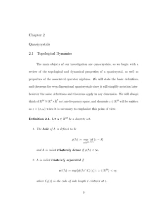
Definition 2.2. Let Λ be a Delone set. The sets Br(z) ∩ Λ where z ∈ Λ are called
the r-patches of Λ.
1. If for any fixed r there are only finitely many r-patches up to translation, then
Λ is said to be of finite local complexity (FLC).
2. For an r-patch P and a set A ⊂ R2d
we define
LP (A) = #{z ∈ R2d
| P − z ⊂ A ∩ Λ}.
Thus LP (A) counts the number of times P appears in A. For a sequence of
balls Brk
(z) in R2d
such that rk goes to ∞, we define the patch frequency of
P to be
freq(P, Λ) = lim
k→∞
LP (Brk
− z)
vol(Brk
)
10](https://image.slidesharecdn.com/05183434-a961-4b18-8b90-61b9aa5d0770-150313140236-conversion-gate01/85/Gabor-Frames-for-Quasicrystals-and-K-theory-16-320.jpg)
![if this limit exists uniformly in z and independent of the choice of balls Brk
.
If the patch frequencies exist for all patches P ⊂ Λ then Λ is said to have
uniform cluster frequencies (UCF).
A Delone set is called a quasicrystal if it is FLC and has UCF.
The study of quasicrystals has to a large extent been driven by the study of
electron interactions in aperiodic solids. Given an electron in an aperiodic solid, we
might assume that it will only interact with nearby electrons since the forces drop
off rapidly as distances increase. Thus for the study of electron interactions, it is
natural to treat two quasicrystals Λ and Λ as the same if they contain precisely the
same local patterns. One could formalize this by saying that any r-patch appearing
in Λ also appears as an r-patch in Λ and vice versa, and in this case we say Λ
and Λ are locally isomorphic. For example, any translate Λ − z is clearly locally
isomorphic to Λ. The collection of all quasicrystals which are locally isomorphic to
Λ will be called the hull of Λ (denoted ΩΛ), and this object is useful in studying
the physics of aperiodic solids (see [6]).
Now we present another construction of the hull which demonstrates how ΩΛ
can be given the structure of a topological dynamical system. Given two Delone
sets Λ, Λ , define
R(Λ, Λ ) = sup{r | ∃z ∈ R2d
with ||z|| <
1
r
, Br ∩ (Λ − z) = Λ ∩ Br}.
We can define the distance between Λ and Λ as
d(Λ, Λ ) = min 1,
1
R(Λ, Λ )
.
11](https://image.slidesharecdn.com/05183434-a961-4b18-8b90-61b9aa5d0770-150313140236-conversion-gate01/85/Gabor-Frames-for-Quasicrystals-and-K-theory-17-320.jpg)
![Intuitively, two Delone sets are close if they agree in a large ball around the origin
after a small translation. This defines a metric d on the space of all Delone subsets
of R2d
, and the resulting topology on point sets is known as the local topology.
Definition 2.3. Given a Delone set Λ, the orbit of Λ is OΛ = {Λ − z | z ∈ R2d
}.
The hull ΩΛ is the closure of OΛ in the metric d.
The hull ΩΛ comes with a natural action of R2d
by translation. The following
proposition shows how regularity properties of Λ can be translated into properties
of the dynamical system (ΩΛ, R2d
) :
Proposition 2.1 ([6], [23]). Let Λ be an aperiodic Delone set.
1. Λ is FLC iff ΩΛ is compact.
2. Λ has UCF iff the dynamical system (ΩΛ, R2d
) is minimal and uniquely ergodic.
Thus we see that for any quasicrystal Λ we have an associated dynamical
system (ΩΛ, R2d
) which is compact, minimal, and uniquely ergodic. In fact, we have
an explicit description of the ergodic measure µ using patch frequencies. Given a
patch P in Λ, and V ⊂ R2d
a precompact open set, define the cylinder set
ΩP,V = {Λ ∈ ΩΛ | P − z ⊂ Λ for some z ∈ V }.
The cylinder sets form a basis for the topology on ΩΛ, so it suffices to describe the
ergodic measure for cylinder sets. Fix η(Λ) so that any ball of radius η(Λ) contains
at most one point of Λ. If diam(V ) < η(Λ), then the measure of ΩP,V is given by
µ(ΩP,V ) = V ol(V )freq(P, Γ)
12](https://image.slidesharecdn.com/05183434-a961-4b18-8b90-61b9aa5d0770-150313140236-conversion-gate01/85/Gabor-Frames-for-Quasicrystals-and-K-theory-18-320.jpg)
![where Γ is an element of ΩΛ. Since we can also describe the hull using local isomor-
phism classes, for any Λ ∈ ΩΛ the quantities rel(Λ ) and ρ(Λ ) are equal to rel(Λ)
and ρ(Λ) respectively. Thus we may think of these quantities as associated to the
hull itself, and not just to a particular point set contained in it. Furthermore, the
patch frequencies are also independent of the choice of point set Λ ∈ ΩΛ so that
the patch frequencies and density can be associated to the tiling space as a whole
as well.
While the hull ΩΛ appears naturally from physical considerations, we will con-
sider now a different space which appears more naturally in the context of harmonic
analysis. We would like to think of a quasicrystal Λ as a collection of shifts we can
apply to a function. The shifts might simply be translations (see [27]), but in the
case of Gabor analysis they will be time-frequency shifts. In this vein, we consider
OΛ
trans := {Λ − z | z ∈ Λ},
the collection of Delone sets which are translates of Λ by points in Λ.
Definition 2.4. We define the canonical transversal Ωtrans as the closure of
OΛ
trans in the metric d.
Note that the canonical transversal can also be defined as
Ωtrans = {Λ ∈ ΩΛ | 0 ∈ Λ },
and is a transversal to the action of R2d
on the hull.
Topologically Ωtrans is a Cantor set, and it comes with a measure which, by
13](https://image.slidesharecdn.com/05183434-a961-4b18-8b90-61b9aa5d0770-150313140236-conversion-gate01/85/Gabor-Frames-for-Quasicrystals-and-K-theory-19-320.jpg)
![abuse of notation, we shall also call µ. Given a patch P ⊂ Λ, we can define
ΩP := {Λ ∈ Ωtrans | P − z = Br(0) ∩ Λ for some r ∈ R, z ∈ R2d
}.
The set ΩP contains exactly the point sets in Ωtrans which have the pattern P
centered at the origin. The sets ΩP form a clopen basis for the topology on Ωtrans,
and µ(ΩP ) = freq(P, Λ). The hull ΩΛ is locally the product of Ωtrans and R2d
as
both a topological space and a measure space. By results of Sadun and Williams
we can always realize ΩΛ as a fiber bundle over a torus with Cantor set fibers [33],
however it is not always the case that Ωtrans carries an action of Z2d
so that ΩΛ is
the suspension of Ωtrans. This will be an important point to keep in mind during
Chapter 5.
2.2 Examples
Now we will present two classes of quasicrystals which comprise the most
commonly studied examples: model sets and substitutions. To construct model
sets in Rd
, we first embed Rd
into a higher dimensional Rn
= Rd
× Rn−d
, or more
generally as part of a product Rd
×G where G is a locally compact abelian group.
Denote by p1 and p2 the projections onto the factors Rd
and G respectively. Then
we choose a lattice D ⊂ Rd
×G so that p1 is injective on D and p2(D) is dense in G.
Instead of projecting all of D onto Rd
, we will project only a piece of D, ensuring
that the resulting collection of points in Rd
is a quasicrystal. This is summarized in
the definition below:
Definition 2.5 (Model sets). Consider the space Rd
×G, where G is a locally com-
14](https://image.slidesharecdn.com/05183434-a961-4b18-8b90-61b9aa5d0770-150313140236-conversion-gate01/85/Gabor-Frames-for-Quasicrystals-and-K-theory-20-320.jpg)
![pact abelian group. Fix D ⊂ Rd
×G a discrete cocompact subgroup and W ⊂ G a
relatively compact subset whose boundary has Haar measure 0. Also assume that π1
is injective on D and π2(D) is dense in W. The triple (Rd
, G, D) is known as the
cut and project scheme. We define the model set or cut and project set ΛW
by
ΛW = {π1(d) | d ∈ D, π2(d) ∈ W}.
When x ∈ ΛW , we define x := p2(p−1
1 (x)). The group G is known as the internal
space and Rd
is known as the physical space.
Any model set (except for a lattice) is aperiodic, FLC, and has UCF ( [6], [23]).
In fact, we can calculate the patch frequencies of patterns in ΛW using the cut and
project scheme:
Proposition 2.2 (Corollary 7.3 in [1]). Let Λ be a model set for the cut and project
scheme (Rd
, G, D) and suppose the window W is compact. If P ⊂ ΛW is a finite
subset, we can determine the relative frequency of P as
rel freq(P, ΛW ) =
vol x∈P (W − x )
vol(W)
and we have the equality
freq(P, ΛW ) = Dens(ΛW )rel freq(P, ΛW ).
We can also compute the density of ΛW as Dens(ΛW ) = vol(W)
vol(D)
.
Many interesting examples of model sets can be constructed using objects from
number theory. Consider the number ring Z[ζ8] ⊂ C where ζ8 is a primitive eighth
root of unity. We have an automorphism x → x of Z[ζ8] given by extending the
15](https://image.slidesharecdn.com/05183434-a961-4b18-8b90-61b9aa5d0770-150313140236-conversion-gate01/85/Gabor-Frames-for-Quasicrystals-and-K-theory-21-320.jpg)
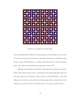
![Figure 2.1: A patch of the Ammann-Beenker tiling.
map ζ8 → ζ3
8 . The map x → (x, x ) gives an embedding of Z[ζ8] as a lattice L8 in
C2 ∼= R4
. We can write L8 =
√
2R8 Z4
where R8 is the rotation matrix
R8 =
1
2
√
2 1 0 −1
0 1
√
2 1
√
2 −1 0 1
0 1 −
√
2 1
.
The projections p1 and p2 are given by projecting onto the first and second copies
of C ∼= R2
respectively. Collectively, we have described a cut and project scheme
(R2
, R2
, L8). The window W will be a regular octagon in R2
centered at the origin
with side length one, and oriented so that all edges are perpendicular to some eighth
root of unity. The resulting model set ΛW is known as the Ammann-Beenker
16](https://image.slidesharecdn.com/05183434-a961-4b18-8b90-61b9aa5d0770-150313140236-conversion-gate01/85/Gabor-Frames-for-Quasicrystals-and-K-theory-22-320.jpg)
![2.3 Poisson Summation Formulas
In studying Gabor analysis on model sets we shall sometimes need to make
use of a generalized Poisson summation formula. Recall that for f ∈ S(Rd
) and a
lattice L ⊂ Rd
the classical Poisson summation states
z∈L
f(z) =
l∈L∗
ˆf(l)
where L∗
denotes the dual lattice
L∗
:= {l ∈ Rd
| l · z ∈ Z for all z ∈ L}.
We can consider the translation bounded measure δL := z∈L δz where δz is the
Dirac delta function at z. Then we can rephrase the Poisson summation formula as
an equality of measures
δL = δL∗ .
Thus if we want an analogous formula for a quasicrystal Λ, we can begin by consid-
ering the measure
δΛ :=
z∈Λ
δz
and try to compute δΛ. Unfortunately, this computation is complicated by the fact
that although δΛ is a measure, δΛ will not be a measure in general. In fact there are
rather stringent restrictions on when this can occur.
Theorem 2.1 ([21] Theorem 3.7). Suppose that Λ and Λ are discrete sets in Rd
,
that {c(l) | l ∈ Λ } are positive numbers, and that the two distributions
f1 =
z∈Λ
δz, f2 =
l∈Λ
c(l)δl
19](https://image.slidesharecdn.com/05183434-a961-4b18-8b90-61b9aa5d0770-150313140236-conversion-gate01/85/Gabor-Frames-for-Quasicrystals-and-K-theory-25-320.jpg)
![are tempered distributions. If f2 = ˆf1, then Λ is a full rank lattice in Rd
, Λ is the
dual lattice, and all c(l) = 1
vol(Λ)
.
Thus we must be very careful while computing δΛ.
For the remainder of the section we will assume that Λ ⊂ Rd
is a model set
with cut and project scheme (Rd
, Rn
, D). We have assumed that the internal space
is Rn
largely for convenience, and all results carry over to the more general case
([34]). We define the dual cut and project scheme to be (Rd
, Rn
, D∗
) and for
convenience we denote p1 and p2 as the projections for both the original cut and
project scheme and its dual. We fix a relatively compact window W and consider
the model set ΛW . For a point k ∈ Rd
, we define the Fourier-Bohr coefficient at
k to be
ck := lim
R→∞
Dens(ΛW )
|ΛW ∩ BR| z∈ΛW ∩BR
e−2πikz
.
For model sets this limit exists independently of the center of the ball BR ([1] Prop
9.9). When k /∈ p1(D∗
) we have ck = 0. It is possible to have ck = 0 even though
k ∈ p1(D∗
), however for model sets such k form a discrete subset of p1(D∗
). One
can see this by computing the Fourier-Bohr coefficients using the Fourier transform
of the characteristic function of the window, as in [1].
A cursory computation of δΛW
shows that ([16] Section 5)
δΛW
=
k∈p1(D∗)
ckδk.
However, since the RHS of this expression is not locally absolutely summable, we
need a more precise way to interpret this sum. To do this, we consider a sequence
of smooth functions ϕ on W such that lim →0 ϕ = χW , the characteristic function
20](https://image.slidesharecdn.com/05183434-a961-4b18-8b90-61b9aa5d0770-150313140236-conversion-gate01/85/Gabor-Frames-for-Quasicrystals-and-K-theory-26-320.jpg)
![of W. We define a corresponding collection of measures
δΛW , :=
z∈ΛW
ϕ (z )δz.
It can be shown that
δΛW , =
k∈p1(D∗)
ckδk
where the RHS is locally absolutely summable. Additionally, we have lim →0 ck = ck.
We summarize this by the following theorem, whose proof can be found in [8] Section
2:
Theorem 2.2. We have
lim
→0
δΛW , = δΛW
in the sense of tempered distributions. Interpreted in this sense, for any f ∈ S(Rd
)
we have
z∈ΛW
ˆf(z) =
k∈p1(D∗)
ckf(k)
where
ck = lim
R→∞
Dens(ΛW )
|ΛW ∩ BR| z∈ΛW ∩BR
e−2πikz
.
To better motivate the definition of the Fourier-Bohr coefficients, we can give
them a dynamical interpretation. For any point k ∈ Rd
we say that k is an eigen-
value of the dynamical system (ΩΛ, Rd
) with eigenfunction ϕk if ϕk is a measurable
complex valued function on ΩΛ satisfying
ϕk(T − z) = e2πikz
ϕk(T)
21](https://image.slidesharecdn.com/05183434-a961-4b18-8b90-61b9aa5d0770-150313140236-conversion-gate01/85/Gabor-Frames-for-Quasicrystals-and-K-theory-27-320.jpg)
![for all T ∈ ΩΛ and z ∈ Rd
. If an eigenfunction exists for an eigenvalue k then
it is unique up to scaling by a unit complex number. If the eigenfunction is con-
tinuous, we call k a continuous eigenvalue. The continuous eigenvalues make
up the discrete part of the dynamical spectrum. By this, we mean that we can
decompose the joint spectrum of the translation operators on ΩΛ, and that the con-
tinuous eigenfunctions make up the discrete part in this decomposition. When the
continuous eigenfunctions make up the entire spectrum, we say that ΩΛ has pure
discrete spectrum. This is equivalent to saying that the linear span of the con-
tinuous eigenfunctions is dense in L2
(ΩΛ). For the classes of quasicrystals we have
described (namely model sets and substitutions) all eigenfunctions are continuous,
and thus we do not have to draw the distinction between measurable and continu-
ous eigenfunctions. However there are other classes where this distinction becomes
important [20].
Now we can describe the connection between Fourier-Bohr coefficients and
eigenvalues. For a model set Λ, ΩΛ always has pure discrete spectrum and the
collection of eigenvalues is exactly p1(D∗
). In this case, we see that the Fourier-Bohr
coefficient ck is simply the integral of the eigenfunction ϕk over Ωtrans after applying
Birkhoff’s ergodic theorem. We will see the eigenfunctions appear again, along with
the Fourier-Bohr coefficients, when we investigate Hilbert C∗
-module structures and
the Janssen representation in Section 4.4.
22](https://image.slidesharecdn.com/05183434-a961-4b18-8b90-61b9aa5d0770-150313140236-conversion-gate01/85/Gabor-Frames-for-Quasicrystals-and-K-theory-28-320.jpg)
![2.4 The Groupoid C∗
-algebra Aσ
We are now ready to describe our main object of study: the groupoid C∗
-
algebra Aσ associated to Ωtrans. We consider the equivalence relation
RΛ = {(T, T ) ∈ Ωtrans × Ωtrans | T is a translate of T }
and an element of RΛ will be written as (T, T − z) where z ∈ R2d
. We give RΛ a
topology by declaring that a sequence (Tk, Tk −zk) → (T, T −z) iff Tk → T in Ωtrans
and |zk − z| → 0. With this topology, RΛ has the structure of a locally compact,
principal, r-discrete groupoid (see [30]). The unit space of RΛ is given by elements
of the form (T, T). We can compose two elements (T, T − z), (T , T − w) only if
T = T − z, and in this case
(T, T − z) ∗ (T − z, T − z − w) = (T, T − z − w).
This groupoid captures the idea of shifting by exactly the points in Λ. To
see this, note that (Λ, Λ − z) ∈ RΛ iff z ∈ Λ. Thus the orbit of Λ in RΛ is in
correspondence with the points of Λ, and the element (Λ, Λ − z) can be thought
of as a shift by z. This will be made more explicit in Section 4.3, where we will
construct a projective representation of RΛ using time-frequency shifts. Anticipating
this, we will describe the cocycle on RΛ which will be involved in this projective
representation. First, let θ be a 2-cocycle on R2d
. We can use θ to construct a
2-cocycle on RΛ, denoted θΛ, using the formula
θΛ ((T, T − z), (T , T − w)) = θ(z, w).
23](https://image.slidesharecdn.com/05183434-a961-4b18-8b90-61b9aa5d0770-150313140236-conversion-gate01/85/Gabor-Frames-for-Quasicrystals-and-K-theory-29-320.jpg)
![Cocycles of this form will be called standard cocycles, and when it is clear we will
drop the subscript from θΛ and refer to both cocycles as θ. We will be particularly
concerned with the symplectic cocycle σ on R2d
given by
σ(z, w) = e−2πixω
where z = (x, ω) and w = (x , ω ).
Following [30] and [6], we construct a C∗
-algebra from RΛ and a 2-cocycle
θ. To construct the C∗
-algebra Aθ = C∗
(RΛ, θ), we begin with Cc(RΛ), with the
product
f ∗ g(T, T − z) :=
w∈T
f(T, T − w)g(T − w, T − z)θ ((T, T − w), (T − w, T − z))
and involution defined by
f∗
(T, T − z) := f(T − z, T)θ ((T, T − z), (T − z, T))
where z = (x, ω). For the symplectic cocycle σ, the multiplication and involution
can be written as
f ∗ g(T, T − z) :=
w=(x ,ω )∈T
f(T, T − w)g(T − w, T − z)e2πix (ω −ω)
and
f∗
(T, T − z) := f(T − z, T)e2πixω
respectively. We can define a norm on Cc(RΛ) by taking the sup over all the norms
coming from the bounded representations of Cc(RΛ) (see [30] Chapter 2 for details,
or [6] Section 4.1 for a description specific to quasicrystals). After completing Cc(RΛ)
in this norm, we obtain the C∗
-algebra Aθ.
24](https://image.slidesharecdn.com/05183434-a961-4b18-8b90-61b9aa5d0770-150313140236-conversion-gate01/85/Gabor-Frames-for-Quasicrystals-and-K-theory-30-320.jpg)
![For a standard cocycle θ, we can also construct a cocycle on the action groupoid
C(ΩΛ) R2d
, and in this case Aθ is Morita equivalent to the twisted crossed product
C∗
(C(ΩΛ) R2d
, θ) [29]. Since the action of R2d
on ΩΛ is minimal and uniquely
ergodic, both algebras are simple and have a unique normalized trace given by
integrating over the unit space of their respective groupoids. For a function f ∈
Cc(RΛ), the trace is given by
Tr(f) =
Ωtrans
f(T, T)dT,
and after applying Birkhoff’s ergodic theorem we can write
Tr(f) = lim
k→∞
1
|Λ ∩ Ck|
z∈(Λ∩Ck)
f(T − z, T − z)
so that the trace is expressed as an average over the values of f on the orbit of Λ.
For a standard cocycle θ we can compute the K-theory of Aθ by appealing to
the following theorem of Gillaspy [13]:
Theorem 2.3 ([13] Thm. 5.1). Let G be a second countable locally compact Haus-
dorff group acting on a second countable locally compact Hausdorff space X such that
G satisfies the Baum-Connes conjecture with coefficients, and let ωt be a homotopy
of continuous 2-cocycles on the transformation group X G. For any t ∈ [0, 1], the
∗-homomorphism
qt : C∗
r (G X × [0, 1], ω) → C∗
r (G X, ωt),
given on Cc(G X × [0, 1]) by evaluation at t ∈ [0, 1], induces an isomorphism
K∗(C∗
r (G X × [0, 1], ω)) ∼= K∗(C∗
r (G X, ωt)).
25](https://image.slidesharecdn.com/05183434-a961-4b18-8b90-61b9aa5d0770-150313140236-conversion-gate01/85/Gabor-Frames-for-Quasicrystals-and-K-theory-31-320.jpg)
![Theorem 2.3, combined with the Connes-Thom isomorphism and the Morita equiv-
alence between Aθ and C∗
(C(ΩΛ) R2d
, θ), gives
K∗(Aθ) ∼= K∗(C∗
(C(ΩΛ) R2d
, θ)) ∼= K∗(C(ΩΛ) R2d
) ∼= K∗(C(ΩΛ)) ∼= K∗
(ΩΛ).
Theorem 2.3 applies since any cocycle on R2d
is homotopic to the trivial cocycle,
essentially by the straight line homotopy. Unfortunately, the K-theory of ΩΛ can be
quite complicated. In many cases K0
(ΩΛ) will not be finitely generated, and there
are examples where it has torsion [12]. Because of these complexities, it is in general
difficult to see how our module HΛ fits into K0(Aσ). In Section 5, we will show that
when Λ ⊂ R2
is a subset of a lattice these difficulties can be overcome, and an
understanding of how HΛ fits into K0(Aσ) is enough to compute Tr∗(K0(Aσ)).
26](https://image.slidesharecdn.com/05183434-a961-4b18-8b90-61b9aa5d0770-150313140236-conversion-gate01/85/Gabor-Frames-for-Quasicrystals-and-K-theory-32-320.jpg)
![f. Similar to the Fourier transform, the STFT has the following continuous recon-
struction formula:
Proposition 3.1 ([14]). Fix g, γ ∈ L2
(Rd
) s.t. g, γ = 0. Then for all f ∈ L2
(Rd
),
f =
1
g, γ R2d
Vgf(x, ω)MωTxγ dωdx.
A central goal in Gabor analysis is to look for discrete versions of this reconstruction
formula. This idea is expressed through the language of frames.
Definition 3.1. A sequence (ej)j∈J in a separable Hilbert space W is called a frame
if there exist constants A, B > 0 s.t. for all f ∈ W
A||f||2
≤
j∈J
| f, ej |2
≤ B||f||2
.
If A = B then (ej) is called a tight frame, and if A = B = 1 then (ej) is called a
Parseval tight frame.
Any frame (ej) has an associated frame operator S given by
Sf =
j∈J
f, ej ej,
which is the composition of the analysis and synthesis operators
(Cf)j = f, ej
D({aj}j∈J ) =
j∈J
ajej.
We have a (non-unique, non-orthogonal) expansion of f given by
f =
j∈J
f, S−1
ej ej
28](https://image.slidesharecdn.com/05183434-a961-4b18-8b90-61b9aa5d0770-150313140236-conversion-gate01/85/Gabor-Frames-for-Quasicrystals-and-K-theory-34-320.jpg)
![where the elements S−1
ej are known as the dual frame. We also have an associated
Parseval tight frame given by (S−1/2
ej)j∈J .
If we wish to discretize the STFT, we can choose a subset Λ ⊂ R2d
and a
window g and ask whether the set
G(g, Λ) =: {π(z)g | z ∈ Λ}
forms a frame for L2
(Rd
). Such frames are called Gabor frames for Λ. More gen-
erally, we can choose finitely many functions g1, . . . , gN and look for multiwindow
Gabor frames of the form
G(g1, . . . , gN , Λ) := {π(z)gi | i = 1 . . . , N, z ∈ Λ}.
In this case elements of the dual frame will be denoted by ˜giz = S−1
(π(z)gi). When
Λ is a lattice, the dual frame will also have the structure of a Gabor frame given by
G( ˜g1, . . . , ˜gN , Λ) where ˜gi = S−1
gi.
With this background in place, it is natural to ask:
Question 3.1. Given a quasicrystal Λ, can we find functions g1, . . . , gN so that
G(g1, . . . , gN , Λ) is a Gabor frame for Λ?
Much of the work in Gabor analysis has focused on the case where Λ is a lattice.
However, recent results in [15] took a large step towards answering this question not
just for quasicrystals, but for any discrete set Λ. In order to explain their results, it
will be necessary to introduce the modulation spaces Mp
(Rd
).
Definition 3.2. Fix a non-zero g ∈ S(Rd
). For 1 ≤ p ≤ ∞ we define the modula-
29](https://image.slidesharecdn.com/05183434-a961-4b18-8b90-61b9aa5d0770-150313140236-conversion-gate01/85/Gabor-Frames-for-Quasicrystals-and-K-theory-35-320.jpg)
![tion spaces
Mp
(Rd
) := {f ∈ S (Rd
) | Vgf ∈ Lp
(R2d
)}
with the norm ||f||Mp = ||Vgf||p.
Different choices for g give rise to equivalent norms on Mp
(Rd
). The modula-
tion space M1
(Rd
) consists of good windows for Gabor analysis. When g ∈ M1
(Rd
)
the analysis and synthesis operators for a Gabor system G(g, Λ) are bounded be-
tween Mp
(Rd
) and lp
(Λ) :
||CΛ
g f||lp ≤ rel(Λ)||g||M1 ||f||Mp
||DΛ
g c||Mp ≤ rel(Λ)||g||M1 ||c||lp .
A Gabor system G(g, Λ) with g ∈ M1
(Rd
) will be called an Mp
-frame if CΛ
g is
bounded below on Mp
(Rd
). This is equivalent to having constants A, B so that for
all f ∈ Mp
(Rd
)
√
A||f||Mp ≤ ||SΛ
g f||Mp ≤
√
B||f||Mp .
In this case the frame operator SΛ
g is invertible on Mp
(Rd
).
Now we are ready to state the result from [15] which gives sufficient conditions
for answering Question 3.1. For g ∈ M1
(Rd
) and δ > 0, we can define the M1
modulus of continuity of g as
ωδ(g) = sup
|z−w|≤δ
||π(z)g − π(w)g||M1
It is clear that ωδ → 0 as δ → 0 since the representation π is strongly continuous in
B(M1
(Rd
)).
30](https://image.slidesharecdn.com/05183434-a961-4b18-8b90-61b9aa5d0770-150313140236-conversion-gate01/85/Gabor-Frames-for-Quasicrystals-and-K-theory-36-320.jpg)
![Theorem 3.1 ( [15]). For g ∈ M1
(Rd
) with ||g||2 = 1 choose δ > 0 so that ωδ(g) < 1.
If Λ ⊂ R2d
is relatively separated and ρ(Λ) < δ, then G(g, Λ) is a Gabor frame for
L2
(Rd
).
From this result, we can see that when ρ(Λ) is small enough there will be many
windows g for which G(g, Λ) is a Gabor frame. Furthermore, when g is one of these
admissible windows, G(g, Λ ) will also form a Gabor frame for any Λ ∈ ΩΛ since
ρ(Λ ) = ρ(Λ). However, when ρ(Λ) is large we cannot expect G(g, Λ) to form a
Gabor frame for any g. In fact, the Balian-Low theorem for non-uniform frames
proven in [15] shows that if G(g, Λ) is a frame then Dens(Λ) > 1. In this case, we
can only expect a multiwindow Gabor frame to exist.
Finally, we will need to introduce one more function space needed for the
proofs in Section 3.2. The Wiener amalgam space W(L∞
, L1
)(Rd
) consists of all
functions f ∈ L∞
(Rd
) such that
||f||W(L∞,L1) :=
k∈Zd
||f||L∞([0,1]d+k) < ∞.
It is a standard result (see [14] Proposition 12.1.11) that when g ∈ M1
(Rd
) then
for any f ∈ M1
(Rd
), Vgf ∈ W(L∞
, L1
)(R2d
) and ||Vgf||W(L∞,L1) ≤ C||f||M1 ||g||M1 .
Also note that if f ∈ W(L∞
, L1
)(Rd
) and T ⊂ Rd
is a Delone set then we have the
inequality
t∈T
|f(t)| ≤ rel(T)||f||W(L∞,L1). (3.1)
If T ∈ ΩΛ then the bound in this inequality is independent of T since rel(T) = rel(Λ).
31](https://image.slidesharecdn.com/05183434-a961-4b18-8b90-61b9aa5d0770-150313140236-conversion-gate01/85/Gabor-Frames-for-Quasicrystals-and-K-theory-37-320.jpg)
![since the vector z −c may lie in Λ−Λ. To fix this, note that we do not need to place
a point exactly in the center of the hole, but only very close to the center, in order
to reduce the hole by a significant amount. Thus if z −c ∈ Λ−Λ, we instead choose
a point c close enough to c so that z − c /∈ Λ − Λ and the hole in P is reduced by
a factor of 2 − η for some small η. We can find such a point c since Λ FLC implies
that Λ − Λ is discrete.
Proposition 3.2. Given a Delone set Λ ⊂ R2d
with FLC and g ∈ M1
(Rd
), we can
find a multiwindow Gabor frame for Λ where the windows consist of time frequency
translates of g. Furthermore, this multiwindow Gabor frame will be an Mp
-frame for
all p.
Proof. Choose δ > 0 so that ωδ(g) < 1. Applying Lemma 3.1, we can find Λ =
N
i=1(Λ + zi) so that ρ(Λ ) < δ. Then by Theorem 1.1,
G(g, Λ ) =
N
i=1
{π(z + zi)g | z ∈ Λ}
is a Gabor frame and by Theorem 5.1 of [15] it is an Mp
-frame for all p. This is
almost equal to the multiwindow Gabor system given by
N
i=1
G(π(zi)g, Λ) =
N
i=1
{π(z)π(zi)g | z ∈ Λ} =
N
i=1
{e−2πixωi
π(z + zi)g | z ∈ Λ}
where z = (x, ω) and zi = (xi, ωi). The functions in the two Gabor systems differ
only by phase factors, so N
i=1 G(π(zi)g, Λ) will satisfy the same frame inequalities
as G(g, Λ ) and thus N
i=1 G(π(zi)g, Λ) is a multiwindow Gabor frame with the same
frame bounds (and Mp
-frame bounds) as G(g, Λ ).
33](https://image.slidesharecdn.com/05183434-a961-4b18-8b90-61b9aa5d0770-150313140236-conversion-gate01/85/Gabor-Frames-for-Quasicrystals-and-K-theory-39-320.jpg)
![Proof. Fix f ∈ L2
(Rd
). On the one hand we have
ST
π(w)f =
N
i=1 z∈T
π(w)f, π(z)gi π(z)gi =
N
i=1 z∈T
e2πix ω
f, π(z − w)gi π(z)gi.
where z = (x, ω) and w = (x , ω ). On the other hand we have
π(w)ST−w
f =
N
i=1 z∈T
f, π(z − w)gi π(w)π(z − w)gi
=
N
i=1 z∈T
e2πix ω
f, π(z − w)gi π(z)gi
and so the two expressions are equal.
We would also like to know something about the continuity of the frame oper-
ators over ΩΛ. If Tk → T in ΩΛ, we cannot expect STk → ST
in the operator norm.
However, we do have that STk → ST
in the strong operator topology.
Proposition 3.4. Suppose Tk → T in ΩΛ and the window functions g1, . . . , gN lie
in M1
(Rd
). Then STk → ST
in the strong operator topology on B(M1
(Rd
)).
Proof. Fix f ∈ M1
(Rd
). Let A = max{||gi||M1 }. Fix > 0 and choose a large cube
C so that for all i
a∈Zn
C
||Vgi
f||L∞([0,1]n+a) <
4ANrel(Λ)
where N is the number of windows in the multiwindow frame. Since Tk → T, we
can choose K so that for all k ≥ K, Tk agrees with T on the cube C up to a small
translation, so that
N
i=1 z∈T∩C
f, π(z)gi π(z)gi −
N
i=1 z∈Tk∩C
f, π(z)gi π(z)gi
M1
<
2
.
35](https://image.slidesharecdn.com/05183434-a961-4b18-8b90-61b9aa5d0770-150313140236-conversion-gate01/85/Gabor-Frames-for-Quasicrystals-and-K-theory-41-320.jpg)
![Then for all k ≥ K we have
||ST
f − STk
f||M1 ≤
N
i=1 z∈TC
f, π(z)gi π(z)gi −
N
i=1 z∈TkC
f, π(z)gi π(z)gi
M1
+
2
≤ A
N
i=1 z∈TC
| f, π(z)gi | +
N
i=1 z∈TkC
| f, π(z)gi |
+
2
= A
N
i=1 z∈TC
|Vgi
f(z)| +
N
i=1 z∈TkC
|Vgi
f(z)|
+
2
≤ 2Arel(Λ)
N
i=1 a∈Zn
C
||Vgi
f||L∞([0,1]n+a)
+
2
< 2ANrel(Λ)
4ANrel(Λ)
+
2
= .
In the fourth inequality it is important to note that the inequality (3.1) holds not
only for the norms, but also for the partial sums. The main reason this proof works
is that rel(T) is constant on ΩΛ. By applying inequality (3.1), this implies that we
can find a cube C so that the sum ST
f is arbitrarily small outside of C independent
of T ∈ ΩΛ.
Even though the mapping T → ST
will not be continuous when B(M1
(Rd
)) is
given the norm topology, we can still show that all the frames G(g1, . . . , gN , T) have
the same optimal frame bounds.
Proposition 3.5. Suppose G(g1, . . . , gN , T) is a frame for each T ∈ ΩΛ and each
gi ∈ M1
(Rd
). For any T ∈ ΩΛ the optimal upper and lower frame bounds for
G(g1, . . . , gN , T) are the same as those for G(g1, . . . , gN , Λ). As a result, ||ST
||M1 =
||SΛ
||M1 and ||(ST
)−1
||M1 = ||(SΛ
)−1
||M1 where || · ||M1 denotes the operator norm
on B(M1
(Rd
)).
36](https://image.slidesharecdn.com/05183434-a961-4b18-8b90-61b9aa5d0770-150313140236-conversion-gate01/85/Gabor-Frames-for-Quasicrystals-and-K-theory-42-320.jpg)
![Note the difference between Corollary 3.1 and Corollary 3.2. Corollary 3.1 says that
there exist windows {gi}N
i=1 ⊂ M1
(Rd
) so that G(g1, . . . , gN , T) is a Gabor frame for
any T ∈ ΩΛ. Corollary 3.2 says that when G(g1, . . . , gN , Λ) is a multiwindow Gabor
frame and each gi ∈ M1
(Rd
), then G(g1, . . . , gN , T) is automatically also a Gabor
frame for any T ∈ ΩΛ. The similarity between the Delone sets in ΩΛ is the key to
Proposition 3.4 which drives all of our results.
3.3 Comparison of Convergence Properties
It is interesting to compare our Proposition 3.4 to the results in [15]. They
define a notion of convergence for point sets which is seemingly much stronger than
the local topology defined in Section 2.1. For Λ ⊂ R2d
a Delone set, they consider
a sequence of Delone sets {Λn | n ≥ 1} produced as follows. For each n ≥ 1 let
τn : Λ → R2d
be a map and define Λn := τn(Λ) = {τn(λ) | λ ∈ Λ}. We assume
τn(λ) → λ as n → ∞. The sequence of sets Λn together with the maps τn is called
a deformation of Λ. We will say that a sequence of sets Λn is a deformation of Λ
with the understanding that the maps τn are also given.
Definition 3.3. A deformation of Λ is called Lipschitz, denoted by Λn
Lip
→ Λ, if:
1. Given R > 0,
sup
λ,λ ∈Λ
|λ−λ |≤R
|(τn(λ) − τn(λ )) − (λ − λ )| → 0 as n → ∞.
2. Given R > 0 there exists R > 0 and n0 ∈ N such that if |τn(λ) − τn(λ) | ≤ R
for some n ≥ n0 and some λ, λ ∈ Λ then |λ − λ | ≤ R .
38](https://image.slidesharecdn.com/05183434-a961-4b18-8b90-61b9aa5d0770-150313140236-conversion-gate01/85/Gabor-Frames-for-Quasicrystals-and-K-theory-44-320.jpg)
![Conjecture 3.2. Suppose Λn ∈ Ωtrans and Λn
Lip
→ Λ. Then the sequence Λn is
eventually constant and equal to Λ.
These conjectures seem reasonable in light of the fact that a local isomorphism
between two quasicrystals need not imply global similarity. However, there is one
class of point sets where local similarity does imply a kind of global similarity. In [2]
the authors show that model sets which are close in the local topology are statisti-
cally similar in the following sense. Let Λ be a model set and suppose Λ ∈ ΩΛ and
Λ agrees with Λ on a large ball around the origin so that d(Λ, Λ ) < . Then there is
a constant C independent of Λ, Λ so that dens(Λ ∆ Λ ) < C . Here dens(Λ) denotes
the upper density of a point set Λ and ∆ denotes the symmetric difference. Further-
more, they show that this property characterizes model sets among quasicrystals.
It is unclear whether this statistical similarity is enough to construct a counterex-
ample to either conjecture. It would be interesting to see whether these conjectures
have different answers depending on the class of quasicrystals (e.g. model set or
substitution) under consideration.
40](https://image.slidesharecdn.com/05183434-a961-4b18-8b90-61b9aa5d0770-150313140236-conversion-gate01/85/Gabor-Frames-for-Quasicrystals-and-K-theory-46-320.jpg)
![Chapter 4
Constructing Aσ-modules
4.1 Lattice Gabor Frames and Modules over Noncommutative Tori
To motivate our construction of modules over Aσ, we will review Rieffel’s
results in [31] on constructing modules over noncommutative tori and relate them
to Gabor analysis as in [25], [26].
Definition 4.1. Let L ⊂ R2d
be a lattice. The C∗
-algebra AL generated by the
time-frequency shifts {π(z) | z ∈ L} is called a noncommutative torus.
We can also define noncommutative tori as twisted convolution algebras. We take
l1
(L) with twisted convolution
a ∗ b(l) :=
µ∈L
a(µ)b(l − µ)σ(µ, l − µ)
where σ is the symplectic cocycle on R2d
. This is equivalent to taking the twisted
group algebra Aθ = C∗
r (Z2d
, θ) where θ = σ|L. The group algebra is generated
by unitaries Un which correspond to the Dirac δ-functions at the elements of Z2d
.
Any cocycle on Z2d
is given by a skew symmetric matrix Θ which describes the
commutation relations between the Un :
UnUm = e2πintΘm
UmUn.
When the off diagonal entries of this matrix are all irrational and rationally inde-
pendent, we call the cocycle totally irrational. The standard trace on Aθ is given
41](https://image.slidesharecdn.com/05183434-a961-4b18-8b90-61b9aa5d0770-150313140236-conversion-gate01/85/Gabor-Frames-for-Quasicrystals-and-K-theory-47-320.jpg)
![by
TrAθ
n∈Z2d
anUn
= a0.
When θ is totally irrational the map TrAθ∗ : K0(Aθ) → R is injective, although in
general it will not be [9].
Each of these definitions of the noncommutative torus comes with its own
advantages. By viewing a noncommutative torus as a twisted group algebra Aθ we
can easily compute its K-theory. Any skew symmetric matrix Θ is homotopic to
the zero matrix by the straight line homotopy, so Theorem 2.3 applies1
and shows
K∗(Aθ) ∼= K∗
(T2d
). On the other hand, when we have a lattice L such that σ|L = θ,
the algebra AL
∼= Aθ and describes Aθ in a specific representation. Rieffel’s insight
was that different lattices can produce different representations of Aθ, and that these
representations exhaust the classes in K0(Aθ).
More precisely, we define the smooth noncommutative torus
A∞
L :=
z∈L
azπ(z) ∈ AL | az decays faster than any polynomial ,
and the analogous smooth subalgebra of Aθ is defined similarly. The algebra A∞
L is
a spectrally invariant subalgebra of AL. There is a canonical action of A∞
L on S(Rd
)
by time-frequency shifts, and we denote this A∞
L -module by VL. We have
TrAL∗([VL]) = vol(L) =
1
Dens(L)
,
and this last equality already suggests how the dimension of this module will gen-
eralize to quasicrystals. We identify a lattice L with a linear map A such that
1
There are many ways to compute the K-theory of noncommutative tori, but we use Theorem
2.3 since we will need this specific isomorphism later.
42](https://image.slidesharecdn.com/05183434-a961-4b18-8b90-61b9aa5d0770-150313140236-conversion-gate01/85/Gabor-Frames-for-Quasicrystals-and-K-theory-48-320.jpg)
![A Z2d
= L. If we fix a cocycle θ then σ|L = θ exactly when A∗
σ = θ.
Theorem 4.1 (Rieffel [31]). Fix a cocycle θ on Z2d
. Any invertible linear map A
such that A∗
σ = θ gives rise to an A∞
θ -module VA Z2d . These modules are finitely
generated and projective, and any class in K0(A∞
θ ) can be represented as [VA Z2d ] for
some A.
In order to promote VL from an A∞
L -module to an AL-module we first endow
it with the structure of a Hilbert C∗
-module. For f, g ∈ S(Rd
), we define an A∞
L
valued inner product by
L f, g :=
z∈L
f, π(z)g π(z).
To prove that this inner product makes VL into a Hilbert A∞
L -module, we must
show (among other, easier identities) that the inner product L f, f always yields a
positive element of A∞
L . It suffices to show that for any g ∈ S(Rd
) we have
L f, f g, g ≥ 0.
Simplifying the right hand side, we have
L f, f g, g =
z∈L
f, π(z)f π(z)g, g =
1
vol(L) l∈L◦
f, π(l)g π(l)g, f ≥ 0
where
L◦
:=
0 −I
I 0
L∗
is the adjoint lattice. Here the second equality follows from an application of the
Poisson summation formula.
43](https://image.slidesharecdn.com/05183434-a961-4b18-8b90-61b9aa5d0770-150313140236-conversion-gate01/85/Gabor-Frames-for-Quasicrystals-and-K-theory-49-320.jpg)
![After doing this, we can consider the canonical Hilbert module structure on A∞
L · Pg
which is given by
a, b = aPgb∗
.
We can use the analysis and synthesis operators to translate this inner product into
an inner product on VL, and this defines a new C∗
-inner product given by
g
L f, h =
z∈L
f, S−1
g π(z)h π(z).
Using this inner product, we have again that Pg = g
L g, g . We can see that this
inner product is equivalent to our original one since
g
L f, h =
z∈L
f, S−1
g π(z)h π(z) =
z∈L
S
−1
2
g f, S
−1
2
g π(z)h π(z) =L S
−1
2
g f, S
−1
2
g h .
Thus we see that g
L g, g is a projection iff L S
−1
2
g g, S
−1
2
g g is a projection iff S
−1
2
g g
generates a Parseval tight frame. Here the last equivalence comes from Theorem 3.3
in [26].
We can see from the previous discussion that when f and g generate Gabor
frames for L, the inner products f
L · , · and g
L · , · are equal iff Sf = Sg, though
they are always isomorphic as Hilbert module structures. We can define an equiva-
lence relation on functions f, g ∈ S(Rd
) by saying f ∼ g iff SL
f = SL
g . We call such
functions L frame equivalent.
Question 4.1. Can we classify functions up to L frame equivalence?
This question is posed as an attempt to understand what types of frame oper-
ators are possible for a lattice L. Note that if f and g generate Parseval tight Gabor
47](https://image.slidesharecdn.com/05183434-a961-4b18-8b90-61b9aa5d0770-150313140236-conversion-gate01/85/Gabor-Frames-for-Quasicrystals-and-K-theory-53-320.jpg)
![frames for L then they are L frame equivalent. We have a characterization of such
functions called the Wexler-Raz orthogonality relations which say that G(g, L)
is a Parseval tight frame iff g, π(l)g = 1
vol(L)
δL◦,0. Thus we can already see the level
of complexity inherent in Question 4.1 by examining Parseval tight frames. Given
the connection between frame equivalence and equality of the Hilbert inner prod-
ucts f
L · , · and g
L · , · , it would be interesting to see whether operator algebraic
techniques could be used to tackle Question 4.1.
In the previous discussion we have used Gabor frames to construct projec-
tions, and then projections to construct Hilbert module structures. However, it
can be advantageous to work in the opposite direction as well. For example, when
vol(L) ≥ 1, we can never construct a single window Gabor frame for L. Regardless,
we will always have a Hilbert bimodule structure on VL. As in the proof of Propo-
sition 3.3 in [31], we can always find a finite collection {gi}N
i=1 ⊂ M1
(Rd
) so that
N
i=1{gi, gi}L◦ = 1A◦
L
. After unpacking the definitions, we see that this is precisely
the condition that G(g1, . . . , gN , L) is a Parseval tight multiwindow Gabor frame.
Thus we have proven the existence of Parseval tight multiwindow Gabor frames for
L using purely operator algebraic machinery! This result was first proven in [25]
using these methods, but now has purely analytic proofs. Nonetheless, it still shows
the benefits of using operator algebras to study Gabor systems.
48](https://image.slidesharecdn.com/05183434-a961-4b18-8b90-61b9aa5d0770-150313140236-conversion-gate01/85/Gabor-Frames-for-Quasicrystals-and-K-theory-54-320.jpg)
![To see that Gi ∈ AL1
σ , we compute
RΛ
|Gi| =
Ωtrans z∈T
f(T), ˜gi
T
z dT
=
Ωtrans z∈T
(ST
)−1
f(T), π(z)gi dT
which holds since ST
is self-adjoint. For convenience we denote by FT the function
(ST
)−1
f(T). Since ST
is invertible in B(M1
(Rd
)) we have FT ∈ M1
(Rd
). Now we
have
Ωtrans z∈T
| FT , π(z)gi | dT =
Ωtrans z∈T
|Vgi
FT (z)|dT
≤ rel(Λ)
Ωtrans
||Vgi
FT ||W(L∞,L1)dT
≤ C rel(Λ)||gi||M1
Ωtrans
||FT ||M1 dT
≤ C rel(Λ) ||gi||M1
Ωtrans
||(ST
)−1
||M1 ||f(T)||M1 dT < ∞
The inequality in the third line comes from Proposition 12.1.11 in [14], and the
constant C is independent of T. We see the integral is finite because the continuity
of f implies ||f(T)||M1 is bounded on Ωtrans, and because Proposition 3.5 shows that
||(ST
)−1
|| = ||(SΛ
)−1
|| for all T.
Proposition 4.1. The map C is a map of AL1
σ -modules.
Proof. First note that the transversally constant functions CΛ are cyclic in HΛ under
the action of AL1
σ . For example, we can get all transversally locally constant functions
by applying characteristic functions of the unit space of RΛ, and locally constant
functions are dense in C(Ωtrans, M1
(Rd
)). Thus it will suffice to prove that C is an
AL1
σ -module map when AL1
σ acts on CΛ.
51](https://image.slidesharecdn.com/05183434-a961-4b18-8b90-61b9aa5d0770-150313140236-conversion-gate01/85/Gabor-Frames-for-Quasicrystals-and-K-theory-57-320.jpg)
![use Proposition 3.3 to rewrite ˜gi
Λ−z
(0,0) as
˜gi
Λ−z
(0,0) = (SΛ−z
)−1
gi = (SΛ−z
)−1
T−xM−ωMωTxgi = T−xM−ω(SΛ
)−1
π(z)gi.
Now we can rewrite the sum as
Tr(P) = lim
k→∞
1
N|Λ ∩ Ck|
N
i=1 z∈(Λ∩Ck)
gi, T−xM−ω(SΛ
)−1
π(z)gi
= lim
k→∞
1
N|Λ ∩ Ck|
N
i=1 z∈(Λ∩Ck)
π(z)gi, ˜gi
Λ
z
which involves only the Gabor frame G(g1, . . . , gN , Λ) and its dual. These averages
coincide precisely with the frame measure introduced in [3]. In Theorem 4.2 (b)
they show that for a single window frame, the averages above are equal to 1
Dens(Λ)
.
Their results are easily generalized to show that this also holds for multiwindow
frames, so we get the following result:
Corollary 4.1. The dimension of HΛ is equal to 1
Dens(Λ)
.
Thus we have completed the proof of Theorem 1.2. Note that the realization of the
frame measure as the dimension of a projective module gives a structural reason
why it should be independent of the choice of windows for the frame.
4.4 Hilbert C∗
-module Structure
In Section 4.1 we saw that it was advantageous to give VL the structure of a
Morita equivalence bimodule. Understanding the structure of End0
A∞
L
VL was partic-
ularly useful as it could be used to derive the Janssen representation of the frame
operator. Motivated by this example, we would like to give HΛ the structure of
54](https://image.slidesharecdn.com/05183434-a961-4b18-8b90-61b9aa5d0770-150313140236-conversion-gate01/85/Gabor-Frames-for-Quasicrystals-and-K-theory-60-320.jpg)
![a Hilbert C∗
-module and study the endomorphism algebra End0
AL1
σ
HΛ, which for
brevity we will denote by BL1
σ . We denote its completion to a C∗
-algebra by Bσ.
In the previous section we showed that HΛ is a finitely generated projective
module. When G(g1, . . . , gN , Λ) is a multiwindow Gabor frame, we constructed an
associated projection2
P ∈ MN (AL1
σ ) which represents [HΛ] in K0(Aσ). In principal,
the projection P can be used to give HΛ an AL1
σ -valued inner product. We can also
use P to describe BL1
σ , though this description does not immediately identify BL1
σ
as a familiar algebra (e.g. it is unclear whether BL1
σ is a twisted groupoid algebra
associated to a quasicrystal Λ ).
We now outline our strategy in greater detail. We can identify the module
HΛ with (AL1
σ )N
P where AL1
σ acts by multiplication on the left. The isomorphism
between HΛ and (AL1
σ )N
P is given by the noncommutative analysis and synthesis
maps. For elements a, b ∈ (AL1
σ )N
P the natural Hilbert C∗
-inner product is given
by
AL1
σ
a, b = aPb∗
.
Using the noncommutative analysis and synthesis operators we can translate this
inner product structure to HΛ. After doing this, we can identify the endomorphism
algebra BL1
σ with P(AL1
σ )N
P acting on (AL1
σ )N
P by multiplication on the right. By
utilizing the noncommutative analysis and synthesis maps we can take an element
of the form PaP where a ∈ (AL1
σ )N
and get an explicit formula for how it acts on
an element in HΛ.
2
Note that the projection P does depend on the choice of window functions g1, . . . , gN , but the
class of P in K0(Aσ) is independent of this choice.
55](https://image.slidesharecdn.com/05183434-a961-4b18-8b90-61b9aa5d0770-150313140236-conversion-gate01/85/Gabor-Frames-for-Quasicrystals-and-K-theory-61-320.jpg)
![a(T, T − z) ∈ AL1
σ , the element PgaPg acts on Ψ ∈ HΛ by
Ψ(PgaPg)(T) =
z∈T
Ψ(T), ˜gT
z
w∈T
e2πix(ω−ω )
a(T − z, T − w)π(w)g
where z = (z, ω), w = (x , ω ). When a(T) is a function on the unit space of RΛ, this
formula simplifies to
z∈T
Ψ(T), ˜gT
z a(T − z)π(z)g.
We can interpret these operators as altering the reconstruction procedure of the
frame G(g, T). If we define
˜τk(T − z, T − w) = e−2πix(ω−ω )
ϕk(T) π(ˇk)π(z)g, ˜gT
w
then we see that the function ˜τk acts on HΛ in exactly the same way as the operator
τk. This demonstrates that τk lies in BL1
σ . To compare with our earlier remarks, note
that ˜τk is a continuous function iff ϕk is a continuous eigenfunction.
Remark 4.1. For a model set with internal space equal to Rn
, the operators τk
generate a noncommutative torus inside Bσ. Because HΛ is finitely generated and
projective, we can complete it to get a type II1 representation of the von Neumann
algebra generated by Aσ. This implies that the representation of the rotation algebra
generated by the τk (which lies in the VN completion of Bσ) completes to a von
Neumann algebra with a faithful, finite trace. This is curious, considering that the
τk act something like time-frequency shifts from a dense subgroup of R2d
. The stan-
dard representation of these time frequency shifts on L2
(Rd
) completes to B(L2
(Rd
))
which has no such trace. This complication was one large obstruction to generalizing
Linnell’s results in [24]. By considering the noncommutative torus generated by the
τk, it may be possible to sidestep this issue and generalize his results.
60](https://image.slidesharecdn.com/05183434-a961-4b18-8b90-61b9aa5d0770-150313140236-conversion-gate01/85/Gabor-Frames-for-Quasicrystals-and-K-theory-66-320.jpg)
![would need to show that TrBσ (τk) = δk,0. This amounts to computing
TrBσ (τk) =
Ωtrans
ϕk(T) π(ˇk)(ST
g )−1
2 g, (ST
g )−1
2 g dT
= lim
R→∞
1
|Λ ∩ Br| z∈Λ∩BR
e2πikz
π(ˇk)(SΛ−z
g )−1
2 g, (SΛ−z
g )−1
2 g
= lim
R→∞
1
|Λ ∩ Br| z∈Λ∩BR
e2πikz
π(z)π(ˇk)(SΛ−z
g )−1
2 g, π(z)(SΛ−z
g )−1
2 g
= lim
R→∞
1
|Λ ∩ Br| z∈Λ∩BR
π(ˇk)(SΛ
g )−1
2 π(z)g, (SΛ
g )−1
2 π(z)g
?
=
1
Dens(Λ)
δk,0
whenever g ∈ M1
(Rd
) generates a Gabor frame for Λ. If Dens(Λ) < 1 then no such
frame will exist, but a similar computation for multiwindow frames would suffice.
To put this in context, when G(g, L) is a Gabor frame for a lattice L, (SL
g )−1
2 g
generates a Parseval tight multiwindow frame. Consequently, when z ∈ L, the
functions (SL
g )−1
2 π(z)g = π(z)(SL
g )−1
2 g all also generate Parseval tight frames. Thus
we have
π(l)(SL
g )−1
2 π(z)g, (SL
g )−1
2 π(z)g = vol(L)δl,0
whenever z ∈ L and l ∈ L◦
by the Wexler-Raz orthogonality relations. So for
lattices, the computation above clearly holds. We also know that the computation
holds for ˇk = 0; this was precisely the computation of the frame measure from [3].
It is possible that an extension of their methods could complete the computation in
full, allowing as to remove the irrationality assumption in Theorem 4.4.
Remark 4.2. To get the equality
TrBσ (τk) =
Ωtrans
ϕk(T) π(ˇk)(ST
)−1
2 g, (ST
)−1
2 g dT
67](https://image.slidesharecdn.com/05183434-a961-4b18-8b90-61b9aa5d0770-150313140236-conversion-gate01/85/Gabor-Frames-for-Quasicrystals-and-K-theory-73-320.jpg)
![K0(C∗
r (Zd
))
i∗
−−−→ K0(A)
∼=
∼=
K0(C∗
r (Zd
×[0, 1], θ))
k∗
−−−→ K0(C∗
r (Zd
Ωtrans × [0, 1], θ))
∼=
∼=
K0(Aθ1 ) −−−→
j∗
K0(Aθ1 )
where the vertical arrows come from the isomorphisms in Theorem 2.3 and the second
horizontal map is induced by the map k : C∗
r (Zd
×[0, 1], θ) → C∗
r (Zd
Ωtrans ×
[0, 1], θ) given by i on the fiber at 0 and the map jt : Aθ(t) → Aθ(t) on the fiber at
0 < t ≤ 1.
Proof. We will prove only the commutativity of the upper square; commutativ-
ity of the lower square follows by a similar argument. Choose a projection P ∈
MN (C∗
r (Zd
)). We can lift this to a path of projections Pt, yielding an element of
K0(C∗
r (Zd
×[0, 1], θ)). When we map this via k∗, we simply extend the projection
on each fiber by making it constant in the Ωtrans direction. Following the maps
the other way around, we can take P and extend it to be constant in the Ωtrans
direction, then lift it to a path of projections. It is clear that k∗(Pt) is one such
possible lift, so we are done.
Theorem 5.1. Let Λ = Zd
be a marked lattice and fix any cocycle θ on Zd
. Then
the maps i∗ and j∗ are injective. We can compare their images with the image of
the canonical map r∗ : K0(C(Ωtrans)) → K0(Aθ) and we find that the intersection is
generated by [1], the class of the rank 1 trivial module.
Remark 5.1. Note that this immediately implies Theorem 1.4, since the map i∗ is
just the noncommutative version of the map p∗
. By a result of Sadun and Williams
71](https://image.slidesharecdn.com/05183434-a961-4b18-8b90-61b9aa5d0770-150313140236-conversion-gate01/85/Gabor-Frames-for-Quasicrystals-and-K-theory-77-320.jpg)
![[33], given any quasicrystal Λ we can find a marked lattice Λ so that ΩΛ and ΩΛ
are homeomorphic. Thus for an arbitrary quasicrystal we can view ΩΛ as a fiber
bundle over a torus, and Theorem 1.4 holds in this case as well.
Proof. First note that when θ is totally irrational, the map Tr∗ ◦j∗ is injective, so j∗
is injective as well. Thus by Proposition 5.1, we see that i∗ must also be injective.
Now let θ be any cocycle. Since i∗ is injective, by Proposition 5.1 we see that j∗
must be as well.
Now we compare the images of i∗ and j∗ with the image of r∗. First suppose θ
is a totally irrational cocycle, and that the intersection of the groups TrAθ∗(K0(Aθ))
and Tr∗(K0(A)) is equal to Z ⊂ R . This is possible since Tr∗(K0(A)) is countable,
so we can simply choose the entries in the matrix for θ to be rationally independent
from Tr∗(K0(A)). Now it is clear that the image of j∗ is disjoint from the projections
in C(Ωtrans) (except for multiples of the identity) since this is true after applying
the trace. Now note that projections in C(Ωtrans) are preserved by the vertical
isomorphisms on the RHS of the diagram in Proposition 5.1, so the same must be
true for i∗. Finally, using the diagram from Proposition 5.1, the theorem holds when
θ is an arbitrary cocycle.
We can interpret the results above in terms of the modules HΛ. When Λ is
a marked lattice, a Gabor frame for Λ is simply a lattice Gabor frame and does
not depend at all on the colorings of the points in Λ. Furthermore, when Λ = Z2d
as a point set then the standard symplectic cocycle σ|Λ is the trivial cocycle. In
this case, we can use the construction of VΛ in Section 4.1 to get a module over
72](https://image.slidesharecdn.com/05183434-a961-4b18-8b90-61b9aa5d0770-150313140236-conversion-gate01/85/Gabor-Frames-for-Quasicrystals-and-K-theory-78-320.jpg)
![C∗
r (Z2d
), and i∗([VΛ]) = [HΛ]. To construct modules over Aθ for general θ, we follow
Rieffel’s construction and apply a linear map A to Λ with A∗
σ = θ. Then we get
a module VΛ over the noncommutative torus AAΛ and j∗([VAΛ]) = [HAΛ]. Thus
our modules precisely describe the images of i∗ and j∗ for even dimensional Λ, and
we can conclude that the twisted gap labeling group for a marked lattice always
contains the image of the trace map on an associated noncommutative torus. With
a little more work, it seems likely that Rieffel’s more general method can be adapted
to construct modules when Λ is odd dimensional as well.
Now we will describe these results in dimension two, where they allow us to
determine the entire gap labeling group. Note that any cocycle θ on Z2
is determined
by a single real number (also denoted θ), which is the only non-zero entry in the
associated skew symmetric matrix. When Λ = Z2
is a marked lattice, we can
compute its K-theory by applying the Pimsner-Voiculescu exact sequence twice, or
by applying the associated Kasparov spectral sequence [18], [36]. In this case we
have
K0(C(Ωtrans) Z2
) = C(Ωtrans, Z)Z2 ⊕ Z
where C(Ωtrans, Z)Z2 denotes the group of coinvariants of the action of Z2
on Ωtrans.
Here the extra copy of Z comes from the inclusion
K0
(T2
) ∼= K0(C∗
r (Z2
)) → K0(C(Ωtrans) Z2
)
of the group algebra of Z2
into C(Ωtrans) Z2
, and the summand C(Ωtrans, Z)Z2
comes from the inclusion
K0(C(Ωtrans)) → K0(C(Ωtrans) Z2
).
73](https://image.slidesharecdn.com/05183434-a961-4b18-8b90-61b9aa5d0770-150313140236-conversion-gate01/85/Gabor-Frames-for-Quasicrystals-and-K-theory-79-320.jpg)
![twisted by standard cocycles. Bellissard’s original (untwisted) gap labeling conjec-
ture could be reduced to the case of marked lattices, essentially by the results of
Sadun and Williams [33]. They show that a quasicrystal Λ can be deformed so that
it is a marked lattice Λ , and that this deformation gives rise to a homeomorphism
between ΩΛ and ΩΛ . Thus we might be tempted to say that we can reduce the
twisted gap labeling conjecture so that it falls within the scope of our results. Un-
fortunately, our results hold only for standard cocycles (i.e. restrictions of cocycles
on R2d
) and in the process of deforming from Λ to Λ we are likely to take a standard
cocycle on Λ to a nonstandard cocycle on Λ . Thus a general computation of the
gap labeling group in dimension two still seems out of reach.
In another direction, our results do not give a full computation of the gap
labeling group in higher dimensions, even for marked lattices with standard cocycles.
We were able to apply linear maps to a marked lattice, and this allowed us to realize
any standard cocycle as the restriction of the symplectic cocycle on R2d
in a number
of different ways. For each linear map with A∗
σ = θ, we got a class in K0(Aθ).
However, linear maps alone are not enough to fill out all the classes in K-theory. A
linear deformation of a marked lattice ignores the colorings of points in the lattice,
essentially avoiding the complexities that make it a quasicrystal.
To summarize, there are two difficulties preventing a more complete compu-
tation of twisted gap labels. First, there is the problem of passing from a general
quasicrystal to a marked lattice, which really has to with extending our results from
standard cocycles to all cocycles. The second problem has to do with finding more
sophisticated deformations of a quasicrystal so that we can represent all classes in
75](https://image.slidesharecdn.com/05183434-a961-4b18-8b90-61b9aa5d0770-150313140236-conversion-gate01/85/Gabor-Frames-for-Quasicrystals-and-K-theory-81-320.jpg)
![K0(Aθ) when the dimension of Λ is greater than two. Actually, it seems reasonable
to hope that a solution to the second problem will also resolve the first. Namely,
we might expect that even given a nonstandard cocycle c we can find a deformation
ϕ so that σ|ϕ(Λ) = c. In fact this was already evident when we were describing the
difficulties in dimension two.
Thus we present the following strategy for improving our results on the twisted
gap labeling. First, we must get a sense of the types of cocycles by which we can
twist. This involves computing the second cohomology group H2
(RΛ, S1
). Ideally
H2
(RΛ, S1
) should be computable in terms of the cohomology of ΩΛ. Next, we fix a
cocycle c and give sufficient conditions for a deformation ϕ to yield the cocycle c on
ϕ(Λ). To expand upon this, we first assume that ϕ(Λ) is a quasicrystal with RΛ
∼=
Rϕ(Λ). Kellendonk has given sufficient conditions on a map ϕ : R2d
→ R2d
which will
ensure this isomorphism of groupoids [19]. Furthermore, we need σ|ϕ(Λ) = c. Once
we have this, Hϕ(Λ) gives a class in K0(Ac) with trace equal to 1
Dens(ϕ(Λ))
. Ideally,
constructing enough maps of this form should exhaust the classes in K0(Ac) and
give us a full computation of the gap labeling group.
76](https://image.slidesharecdn.com/05183434-a961-4b18-8b90-61b9aa5d0770-150313140236-conversion-gate01/85/Gabor-Frames-for-Quasicrystals-and-K-theory-82-320.jpg)
![Appendix A
K-theory for C∗
-algebras
The discussion in these appendices is modeled largely on the explanations of
K-theory in [10], [22]. We begin with some basic facts about C∗
-algebras.
Definition A.1. A C∗
-algebra A is a C-algebra equipped with a norm || · || and
an involution a → a∗
such that A is complete with respect to the norm, ||ab|| ≤
||a|| · ||b||, and ||a∗
a|| = ||a||2
for all a, b ∈ A. Although a C∗
-algebra need not
have a multiplicative identity, all of our examples will. A homomorphism between
C∗
-algebras is a simply a homomorphism of C-algebras which is continuous and
preserves the involution.
C∗
-algebras and Banach algebras differ only by the final condition in the above
definition. Small though it may seem, this additional axiom makes C∗
-algebras
especially amenable to topological techniques.
Example A.1. C itself is a C∗
-algebra, as is any matrix algebra MN (C). Here the
norm is given by the operator norm, and the involution is by conjugate transpose.
Similarly, for any C∗
-algebra A, MN (A) is also a C∗
-algebra. Finally, B(H), the
bounded linear operators on a Hilbert space, is a C∗
-algebra. In fact it can be shown
that any C∗
-algebra embeds as a subalgebra of B(H).
Example A.2. Let L ⊂ R2
be a lattice and consider the family of time-frequency
78](https://image.slidesharecdn.com/05183434-a961-4b18-8b90-61b9aa5d0770-150313140236-conversion-gate01/85/Gabor-Frames-for-Quasicrystals-and-K-theory-84-320.jpg)
![Definition B.2. Let E and F be Hilbert A-modules. A map T : E → F is ad-
jointable if there exists a map T∗
: F → E, called the adjoint of T, such that
F
A r, Ts = E
A T∗
r, s
whenever r ∈ F, s ∈ E.
We shall be primarily concerned with EndA(E), the space of adjointable operators
from E to itself. An important class of adjointable operators is given by the A-finite
rank operators, which are operators of the form A · , r s where r, s ∈ E. The A-
finite rank operators form a vector space denoted by End00
A (E), and the closure of
End00
A (E) will be known as the collection of A-compact operators, denoted by
End0
A.
Example B.3. If P ∈ Pn then An
P is a Hilbert A-module and End0
A(An
P) =
PMn(A)P. See [10] Lemma 2.18 for details.
We can think of A acting on E on the left while B = End0
A acts on E on the
right. Additionally, we can give E the structure of a right Hilbert B-module by
defining the inner product
{r, s}B := A · , r s.
This leads to the definition of a Hilbert A-B bimodule.
Definition B.3. A pre-C∗
A-B-bimodule is a complex vector space E which is
both a left Hilbert A-module and a right Hilbert B-module where the inner products
satisfy the following compatibility condition:
A r, s t = r{s, t}B for all r, s, t ∈ E.
85](https://image.slidesharecdn.com/05183434-a961-4b18-8b90-61b9aa5d0770-150313140236-conversion-gate01/85/Gabor-Frames-for-Quasicrystals-and-K-theory-91-320.jpg)
![Bibliography
[1] M. Baake and U. Grimm. Aperiodic Order Volume 1: A Mathematical Invita-
tion. Encyclopedia of Mathematics and its Applications. Cambridge, 2013.
[2] M. Baake, D. Lenz, and R. Moody. Characterization of model sets by dynamical
systems. Ergodic Theory and Dynamical Systems, 27:341–382, 2007.
[3] R. Balan, P. Casazza, C. Heil, and Z. Landau. Density, Overcompleteness, and
Localization of Frames. II. Gabor Systems. Journal of Fourier Analysis and
Applications, 12:307–344, 2006.
[4] J. Bellissard. The Noncommutative Geometry of Aperiodic Solids. In Geometric
and Topological Methods for Quantum Field Theory, pages 86–156. World Sci.
Publishing, 2003.
[5] J. Bellissard, R. Benedetti, and J.-M. Gambaudo. Spaces of tilings, finite
telescopic approximation and gap labelings. Communications in Mathemati-
cal Physics, 261:1–41, 2006.
[6] J. Bellissard, D.J.L. Herrmann, and M. Zarrouati. Hulls of Aperiodic Solids and
Gap Labelling Theorems. In M. Baake and R. Moody, editors, Directions in
Mathematical Quasicrystals, volume 13 of CRM Monogr. Ser., pages 177–206.
Amer. Math. Soc., 2000.
[7] M. Benameur and H. Oyono-Oyono. Index theory for quasi-crystals I. Compu-
tation of the gap-label group. Journal of Functional Analysis, pages 137–170,
2007.
[8] G. Bernuau and M. Duneau. Fourier Analysis of Deformed Model Sets. In
M. Baake and R. Moody, editors, Directions in Mathematical Quasicrystals,
volume 13 of CRM Monogr. Ser., pages 43–60. Amer. Math. Soc., 2000.
[9] G. Elliott. On the K-theory of the C∗
-algebra generated by a projective rep-
resentation of a torsion-free discrete Abelian group. In Gr. Arsene, S. Str˘atil˘a,
A. Verona, and D. Voiculescu, editors, Operator Algebras and Group Represen-
tations Volume 1. Pitman Advanced Publishing Program, 1980.
[10] H. Figueroa, J. M. Gracia-Bondia, and J. Varilly. Elements of Noncommutative
Geometry. Birkh¨auser, 2001.
[11] A. Forrest and J. Hunton. The cohomology and K-theory of commuting home-
morphisms of the Cantor set. Ergodic Theory and Dynamical Systems, 19:611–
625, 1999.
[12] F. Gahler, J. Hunton, and J. Kellendonk. Integral cohomology of rational
projection method patterns. Algebraic and Geometric Topology, 13:1661–1708,
2013.
87](https://image.slidesharecdn.com/05183434-a961-4b18-8b90-61b9aa5d0770-150313140236-conversion-gate01/85/Gabor-Frames-for-Quasicrystals-and-K-theory-93-320.jpg)
![[13] E. Gillaspy. K-theory and homotopies of 2-cocycles on transformation groups.
2014. Pre-print, arXiv:1402.3280 [math.OA].
[14] K. Gr¨ochenig. Foundations of Time-Frequency Analysis. Birkh¨auser, 2001.
[15] K. Gr¨ochenig, J. Ortega-Cerda, and J. L. Romero. Deformations of Gabor
Systems. 2013. Pre-print, arXiv:1311.3861 [math.FA].
[16] A. Hof. On Diffraction by Aperiodic Structures. Communications in Mathe-
matical Physics, 169:25–43, 1995.
[17] J. Kaminker and I. Putnam. A proof of the gap labeling conjecture. Michigan
Math Journal, 51:537–546, 2003.
[18] G. G. Kasparov. Equivariant KK-theory and the Novikov conjecture. Invent.
math., 91:147–201, 1988.
[19] J. Kellendonk. Pattern equivariant functions, deformations and equivalence of
tiling spaces. Ergodic Theory and Dynamical Systems, 28:1153–1176, 2008.
[20] J. Kellendonk and L. Sadun. Meyer sets, topological eigenvalues, and Cantor
fiber bundles. Preprint arXiv:1211.2250 [math.DS].
[21] J. Lagarias. Mathematical Quasicrystals and the Problem of Diffraction. In
M. Baake and R. Moody, editors, Directions in Mathematical Quasicrystals,
volume 13 of CRM Monogr. Ser., pages 61–93. Amer. Math. Soc., 2000.
[22] F. Larsen, N. Laustsen, and M. Rordam. An Introduction to K-theory for
C∗
-algebras.
[23] J.Y. Lee, R. Moody, and B. Solomyak. Pure Point Dynamical and Diffraction
Spectra. Annales Henri Poincare, 3:1003–1018, 2002.
[24] P. A. Linnell. Von Neumann Algebras and Linear Independence of Translates.
Proceedings of the American Mathematical Society, 127(11):3269–3277, 1999.
[25] F. Luef. Projective modules over noncommutative tori are multi-window Gabor
frames for modulation spaces. Journal of Functional Analysis, 257:1921–1946,
2009.
[26] F. Luef. Projections in noncommutative tori and Gabor frames. Proceedings of
the AMS, 139:571–582, 2011.
[27] B. Matei and Y. Meyer. Simple quasicrystals are sets of stable sampling. Com-
plex Variables and Elliptic Equations, 55:947–964, 2010.
[28] Y. Meyer. Algebraic Numbers and Harmonic Analysis. North-Holland, 1972.
[29] P. Muhly, J. Renault, and D. Williams. Equivalence and Isomorphism for
Groupoid C∗
-Algebras. Journal of Operator Theory, 17, 1987.
88](https://image.slidesharecdn.com/05183434-a961-4b18-8b90-61b9aa5d0770-150313140236-conversion-gate01/85/Gabor-Frames-for-Quasicrystals-and-K-theory-94-320.jpg)
![[30] J. Renault. A Groupoid Approach to C∗
-Algebras, volume 793 of Lecture Notes
in Mathematics. Springer, 1980.
[31] M. Rieffel. Projective modules over higher-dimensional noncommutative tori.
Canadian Journal of Mathematics, 40:257–338, 1988.
[32] L. Sadun. Topology of Tiling Spaces, volume 46 of University Lecture Series.
American Mathematical Society, 2008.
[33] L. Sadun and R. F. Williams. Tiling spaces are Cantor set fiber bundles. Ergodic
Theory and Dynamical Systems, 23:307–316, 2003.
[34] M. Schlottmann. Generalized Model Sets and Dynamical Systems. In M. Baake
and R. Moody, editors, Directions in Mathematical Quasicrystals, volume 13 of
CRM Monogr. Ser., pages 143–159. Amer. Math. Soc., 2000.
[35] D. Shechtman, I. Blech, D. Gratias, and J. Cahn. Metallic Phase with Long-
Range Orientational Order and No Translational Symmetry. Physical Review
Letters, 53:1951–1953, 1984.
[36] A. van Elst. Gap labelling for Schr¨odinger operators on the square and cubic
lattices. Rev. Math. Phys, 6, 1994.
89](https://image.slidesharecdn.com/05183434-a961-4b18-8b90-61b9aa5d0770-150313140236-conversion-gate01/85/Gabor-Frames-for-Quasicrystals-and-K-theory-95-320.jpg)


![[SEMINAR at my uni] Tuesday, 14th May, 2019](https://cdn.slidesharecdn.com/ss_thumbnails/may07seminar19051303-190513213519-240815072320-c3e1932b-thumbnail.jpg?width=640&height=640&fit=bounds)


