Download to read offline
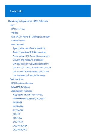


![DAX overview
11/30/2021 • 31 minutes to read
Calculations
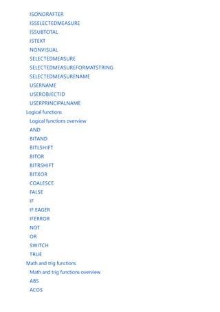
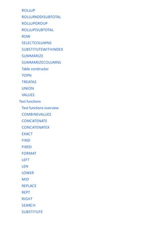
Measures
Total Sales = SUM([Sales Amount])
Data Analysis Expressions (DAX) is a formula expression language used in Analysis Services, Power BI, and
Power Pivot in Excel. DAX formulas include functions, operators, and values to perform advanced calculations
and queries on data in related tables and columns in tabular data models.
This article provides only a basic introduction to the most important concepts in DAX. It describes DAX as it
applies to all the products that use it. Some functionality may not apply to certain products or use cases. Refer to
your product's documentation describing its particular implementation of DAX.
DAX formulas are used in measures, calculated columns, calculated tables, and row-level security.
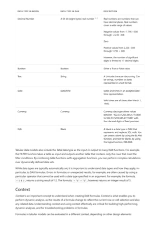
Measures are dynamic calculation formulas where the results change depending on context. Measures are used
in reporting that support combining and filtering model data by using multiple attributes such as a Power BI
report or Excel PivotTable or PivotChart. Measures are created by using the DAX formula bar in the model
designer.
A formula in a measure can use standard aggregation functions automatically created by using the Autosum
feature, such as COUNT or SUM, or you can define your own formula by using the DAX formula bar. Named
measures can be passed as an argument to other measures.
When you define a formula for a measure in the formula bar, a Tooltip feature shows a preview of what the
results would be for the total in the current context, but otherwise the results are not immediately output
anywhere. The reason you cannot see the (filtered) results of the calculation immediately is because the result of
a measure cannot be determined without context. To evaluate a measure requires a reporting client application
that can provide the context needed to retrieve the data relevant to each cell and then evaluate the expression
for each cell. That client might be an Excel PivotTable or PivotChart, a Power BI report, or a table expression in a
DAX query in SQL Server Management Studio (SSMS).
Regardless of the client, a separate query is run for each cell in the results. That is to say, each combination of
row and column headers in a PivotTable, or each selection of slicers and filters in a Power BI report, generates a
different subset of data over which the measure is calculated. For example, using this very simple measure
formula:
When a user places the TotalSales measure in a report, and then places the Product Category column from a
Product table into Filters, the sum of Sales Amount is calculated and displayed for each product category.
Unlike calculated columns, the syntax for a measure includes the measure's name preceding the formula. In the
example just provided, the name Total Sales appears preceding the formula. After you've created a measure,
the name and its definition appear in the reporting client application Fields list, and depending on perspectives
and roles is available to all users of the model.
To learn more, see:
Measures in Power BI Desktop
Measures in Analysis Services](https://image.slidesharecdn.com/funcoesdax-220812141017-bb6cd4dc/85/Funcoes-DAX-pdf-14-320.jpg)
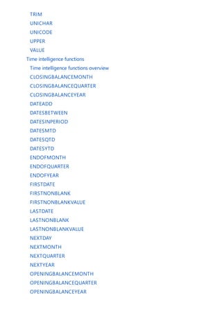
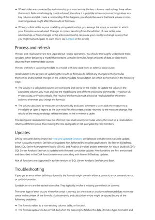
![Calculated columns
= [Calendar Year] & " Q" & [Calendar Quarter]
Calculated tables
Row-level security
= Customers[Country] = "USA"
Measures in Power Pivot
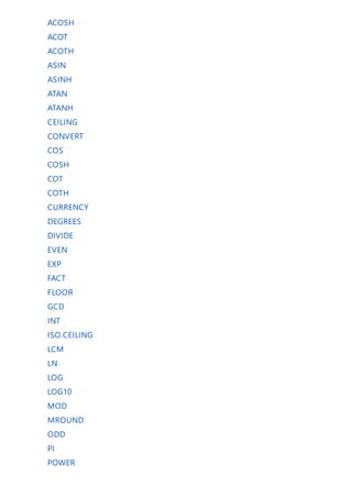
A calculated column is a column that you add to an existing table (in the model designer) and then create a DAX
formula that defines the column's values. When a calculated column contains a valid DAX formula, values are
calculated for each row as soon as the formula is entered. Values are then stored in the in-memory data model.
For example, in a Date table, when the formula is entered into the formula bar:
A value for each row in the table is calculated by taking values from the Calendar Year column (in the same Date
table), adding a space and the capital letter Q, and then adding the values from the Calendar Quarter column (in
the same Date table). The result for each row in the calculated column is calculated immediately and appears, for
example, as 2017 Q1. Column values are only recalculated if the table or any related table is processed
(refresh) or the model is unloaded from memory and then reloaded, like when closing and reopening a Power BI
Desktop file.
To learn more, see:
Calculated columns in Power BI Desktop
Calculated columns in Analysis Services
Calculated Columns in Power Pivot.
A calculated table is a computed object, based on a formula expression, derived from all or part of other tables
in the same model. Instead of querying and loading values into your new table's columns from a data source, a
DAX formula defines the table's values.
Calculated tables can be helpful in a role-playing dimension. An example is the Date table, as OrderDate,
ShipDate, or DueDate, depending on the foreign key relationship. By creating a calculated table for ShipDate
explicitly, you get a standalone table that is available for queries, as fully operable as any other table. Calculated
tables are also useful when configuring a filtered rowset, or a subset or superset of columns from other existing
tables. This allows you to keep the original table intact while creating variations of that table to support specific
scenarios.
Calculated tables support relationships with other tables. The columns in your calculated table have data types,
formatting, and can belong to a data category. Calculated tables can be named, and surfaced or hidden just like
any other table. Calculated tables are re-calculated if any of the tables it pulls data from are refreshed or
updated.
To learn more, see:
Calculated tables in Power BI Desktop
Calculated tables in Analysis Services.
With row-level security, a DAX formula must evaluate to a Boolean TRUE/FALSE condition, defining which rows
can be returned by the results of a query by members of a particular role. For example, for members of the
Sales role, the Customers table with the following DAX formula:
Members of the Sales role will only be able to view data for customers in the USA, and aggregates, such as SUM
are returned only for customers in the USA. Row-level security is not available in Power Pivot in Excel.
When defining row-level secuirty by using DAX formula, you are creating an allowed row set. This does not](https://image.slidesharecdn.com/funcoesdax-220812141017-bb6cd4dc/85/Funcoes-DAX-pdf-15-320.jpg)
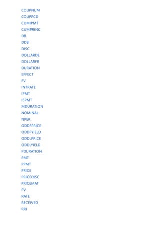
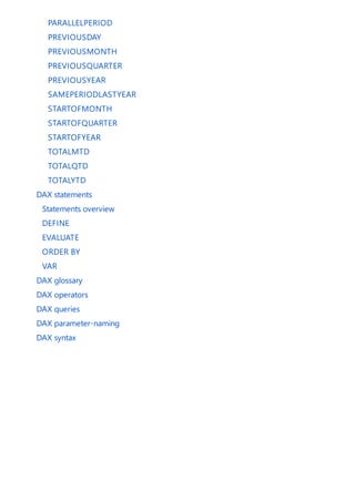
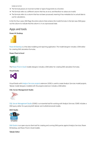
![Queries
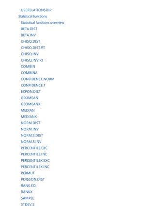
EVALUATE
( FILTER ( 'DimProduct', [SafetyStockLevel] < 200 ) )
ORDER BY [EnglishProductName] ASC
Formulas
Formula basics
FORMULA DEFINITION
= TODAY() Inserts today's date in every row of a calculated column.
= 3 Inserts the value 3 in every row of a calculated column.
= [Column1] + [Column2] Adds the values in the same row of [Column1] and
[Column2] and puts the results in the calculated column of
the same row.
deny access to other rows; rather, they are simply not returned as part of the allowed row set. Other roles can
allow access to the rows excluded by the DAX formula. If a user is a member of another role, and that role's row-
level security allows access to that particular row set, the user can view data for that row.
Row-level security formulas apply to the specified rows as well as related rows. When a table has multiple
relationships, filters apply security for the relationship that is active. Row-level security formulas will be
intersected with other formulas defined for related tables.
To learn more, see:
Row-level security (RLS) with Power BI
Roles in Analysis Services
DAX queries can be created and run in SQL Server Management Studio (SSMS) and open-source tools like DAX
Studio (daxstudio.org). Unlike DAX calculation formulas, which can only be created in tabular data models, DAX
queries can also be run against Analysis Services Multidimensional models. DAX queries are often easier to
write and more efficient than Multidimensional Data Expressions (MDX) queries.
A DAX query is a statement, similar to a SELECT statement in T-SQL. The most basic type of DAX query is an
evaluate statement. For example,
Returns in Results a table listing only those products with a SafetyStockLevel less than 200, in ascending order
by EnglishProductName.
You can create measures as part of the query. Measures exist only for the duration of the query. To learn more,
see DAX queries.
DAX formulas are essential for creating calculations in calculated columns and measures, and securing your data
by using row-level security. To create formulas for calculated columns and measures, use the formula bar along
the top of the model designer window or the DAX Editor. To create formulas for row-level security, use the Role
Manager or Manage roles dialog box. Information in this section is meant to get you started with understanding
the basics of DAX formulas.
DAX formulas can be very simple or quite complex. The following table shows some examples of simple
formulas that could be used in a calculated column.
Whether the formula you create is simple or complex, you can use the following steps when building a formula:](https://image.slidesharecdn.com/funcoesdax-220812141017-bb6cd4dc/85/Funcoes-DAX-pdf-16-320.jpg)
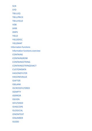
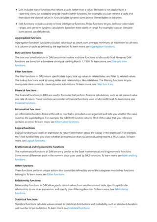
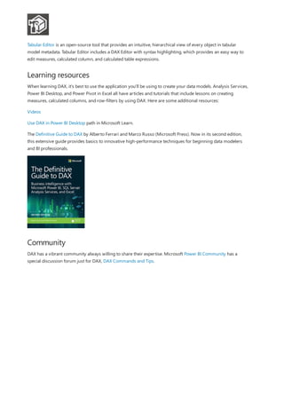
![NOTE
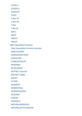
Days in Current Quarter = COUNTROWS( DATESBETWEEN( 'Date'[Date], STARTOFQUARTER( LASTDATE('Date'[Date])),
ENDOFQUARTER('Date'[Date])))
FORMULA ELEMENT DESCRIPTION
Days in Current Quarter The name of the measure.
= The equals sign (=) begins the formula.
COUNTROWS COUNTROWS counts the number of rows in the Date table
() Open and closing parenthesis specifies arguments.
DATESBETWEEN The DATESBETWEEN function returns the dates between the
last date for each value in the Date column in the Date table.
'Date' Specifies the Date table. Tables are in single quotes.
[Date] Specifies the Date column in the Date table. Columns are in
brackets.
1. Each formula must begin with an equal sign (=).
2. You can either type or select a function name, or type an expression.
3. Begin to type the first few letters of the function or name you want, and AutoComplete displays a list of
available functions, tables, and columns. Press TAB to add an item from the AutoComplete list to the
formula.
You can also click the Fx button to display a list of available functions. To select a function from the
dropdown list, use the arrow keys to highlight the item, and click OK to add the function to the formula.
4. Supply the arguments to the function by selecting them from a dropdown list of possible tables and
columns, or by typing in values.
5. Check for syntax errors: ensure that all parentheses are closed and columns, tables and values are
referenced correctly.
6. Press ENTER to accept the formula.
In a calculated column, as soon as you enter the formula and the formula is validated, the column is populated with
values. In a measure, pressing ENTER saves the measure definition with the table. If a formula is invalid, an error is
displayed.
In this example, let's look at a formula in a measure named Days in Current Quarter:
This measure is used to create a comparison ratio between an incomplete period and the previous period. The
formula must take into account the proportion of the period that has elapsed, and compare it to the same
proportion in the previous period. In this case, [Days Current Quarter to Date]/[Days in Current Quarter] gives
the proportion elapsed in the current period.
This formula contains the following elements:](https://image.slidesharecdn.com/funcoesdax-220812141017-bb6cd4dc/85/Funcoes-DAX-pdf-17-320.jpg)
![,
STARTOFQUARTER The STARTOFQUARTER function returns the date of the start
of the quarter.
LASTDATE The LASTDATE function returns the last date of the quarter.
'Date' Specifies the Date table.
[Date] Specifies the Date column in the Date table.
,
ENDOFQUARTER The ENDOFQUARTER function
'Date' Specifies the Date table.
[Date] Specifies the Date column in the Date table.
FORMULA ELEMENT DESCRIPTION
Using formula AutoComplete
Using multiple functions in a formula
Functions
AutoComplete helps you enter a valid formula syntax by providing you with options for each element in the
formula.
You can use formula AutoComplete in the middle of an existing formula with nested functions. The text
immediately before the insertion point is used to display values in the drop-down list, and all of the text
after the insertion point remains unchanged.
AutoComplete does not add the closing parenthesis of functions or automatically match parentheses. You
must make sure that each function is syntactically correct or you cannot save or use the formula.
You can nest functions, meaning that you use the results from one function as an argument of another function.
You can nest up to 64 levels of functions in calculated columns. However, nesting can make it difficult to create
or troubleshoot formulas. Many functions are designed to be used solely as nested functions. These functions
return a table, which cannot be directly saved as a result; it must be provided as input to a table function. For
example, the functions SUMX, AVERAGEX, and MINX all require a table as the first argument.
A function is a named formula within an expression. Most functions have required and optional arguments, also
known as parameters, as input. When the function is executed, a value is returned. DAX includes functions you
can use to perform calculations using dates and times, create conditional values, work with strings, perform
lookups based on relationships, and the ability to iterate over a table to perform recursive calculations. If you are
familiar with Excel formulas, many of these functions will appear very similar; however, DAX formulas are
different in the following important ways:
A DAX function always references a complete column or a table. If you want to use only particular values
from a table or column, you can add filters to the formula.
If you need to customize calculations on a row-by-row basis, DAX provides functions that let you use the
current row value or a related value as a kind of parameter, to perform calculations that vary by context.
To understand how these functions work, see Context in this article.](https://image.slidesharecdn.com/funcoesdax-220812141017-bb6cd4dc/85/Funcoes-DAX-pdf-18-320.jpg)
![Text functions
Time intelligence functions
Table manipulation functions
Variables
VAR
TotalQty = SUM ( Sales[Quantity] )
Return
IF (
TotalQty > 1000,
TotalQty * 0.95,
TotalQty * 1.25
)
Data types
DATA TYPE IN MODEL DATA TYPE IN DAX DESCRIPTION
Whole Number A 64 bit (eight-bytes) integer value Numbers that have no decimal places.
Integers can be positive or negative
numbers, but must be whole numbers
between -9,223,372,036,854,775,808
(-2^63) and
9,223,372,036,854,775,807 (2^63-1).
Text functions in DAX are very similar to their counterparts in Excel. You can return part of a string, search for
text within a string, or concatenate string values. DAX also provides functions for controlling the formats for
dates, times, and numbers. To learn more, see Text functions.
The time intelligence functions provided in DAX let you create calculations that use built-in knowledge about
calendars and dates. By using time and date ranges in combination with aggregations or calculations, you can
build meaningful comparisons across comparable time periods for sales, inventory, and so on. To learn more,
see Time intelligence functions (DAX).
These functions return a table or manipulate existing tables. For example, by using ADDCOLUMNS you can add
calculated columns to a specified table, or you can return a summary table over a set of groups with the
SUMMARIZECOLUMNS function. To learn more, see Table manipulation functions.
You can create variables within an expression by using VAR. VAR is technically not a function, it's a keyword to
store the result of an expression as a named variable. That variable can then be passed as an argument to other
measure expressions. For example:
In this example, TotalQty can be passed as a named variable to other expressions. Variables can be of any scalar
data type, including tables. Using variables in your DAX formulas can be incredibly powerful.
You can import data into a model from many different data sources that might support different data types.
When you import data into a model, the data is converted to one of the tabular model data types. When the
model data is used in a calculation, the data is then converted to a DAX data type for the duration and output of
the calculation. When you create a DAX formula, the terms used in the formula will automatically determine the
value data type returned.
DAX supports the following data types:
1, 2](https://image.slidesharecdn.com/funcoesdax-220812141017-bb6cd4dc/85/Funcoes-DAX-pdf-20-320.jpg)
![Row context
= [Freight] + RELATED('Region'[TaxRate])
Multiple row context
= MAXX(FILTER(Sales,[ProdKey] = EARLIER([ProdKey])),Sales[OrderQty])
Query context
Filters applied in a PivotTable or report
Filters defined within a formula
Relationships specified by using special functions within a formula
There are different types of context: row context, query context, and filter context.
Row context can be thought of as "the current row". If you create a formula in a calculated column, the row
context for that formula includes the values from all columns in the current row. If the table is related to another
table, the content also includes all the values from the other table that are related to the current row.
For example, suppose you create a calculated column, = [Freight] + [Tax] , that adds together values from two
columns, Freight and Tax, from the same table. This formula automatically gets only the values from the current
row in the specified columns.
Row context also follows any relationships that have been defined between tables, including relationships
defined within a calculated column by using DAX formulas, to determine which rows in related tables are
associated with the current row.
For example, the following formula uses the RELATED function to fetch a tax value from a related table, based on
the region that the order was shipped to. The tax value is determined by using the value for region in the current
table, looking up the region in the related table, and then getting the tax rate for that region from the related
table.
This formula gets the tax rate for the current region from the Region table and adds it to the value of the Freight
column. In DAX formulas, you do not need to know or specify the specific relationship that connects the tables.
DAX includes functions that iterate calculations over a table. These functions can have multiple current rows,
each with its own row context. In essence, these functions let you create formulas that perform operations
recursively over an inner and outer loop.
For example, suppose your model contains a Products table and a Sales table. Users might want to go through
the entire sales table, which is full of transactions involving multiple products, and find the largest quantity
ordered for each product in any one transaction.
With DAX you can build a single formula that returns the correct value, and the results are automatically
updated any time a user adds data to the tables.
For a detailed example of this formula, see EARLIER.
To summarize, the EARLIER function stores the row context from the operation that preceded the current
operation. At all times, the function stores in memory two sets of context: one set of context represents the
current row for the inner loop of the formula, and another set of context represents the current row for the outer
loop of the formula. DAX automatically feeds values between the two loops so that you can create complex
aggregates.
Query context refers to the subset of data that is implicitly retrieved for a formula. For example, when a user
places a measure or field into a report, the engine examines row and column headers, slicers, and report filters
to determine the context. The necessary queries are then run against model data to get the correct subset of](https://image.slidesharecdn.com/funcoesdax-220812141017-bb6cd4dc/85/Funcoes-DAX-pdf-22-320.jpg)
![Filter context
Determining context in formulas
data, make the calculations defined by the formula, and then populate values in the report.
Because context changes depending on where you place the formula, the results of the formula can also change.
For example, suppose you create a formula that sums the values in the Profit column of the Sales table:
= SUM('Sales'[Profit]) . If you use this formula in a calculated column within the Sales table, the results for the
formula will be the same for the entire table, because the query context for the formula is always the entire data
set of the Sales table. Results will have profit for all regions, all products, all years, and so on.
However, users typically don't want to see the same result hundreds of times, but instead want to get the profit
for a particular year, a particular country, a particular product, or some combination of these, and then get a
grand total.
In a report, context is changed by filtering, adding or removing fields, and using slicers. For each change, the
query context in which the measure is evaluated. Therefore, the same formula, used in a measure, is evaluated in
a different query context for each cell.
Filter context is the set of values allowed in each column, or in the values retrieved from a related table. Filters
can be applied to the column in the designer, or in the presentation layer (reports and PivotTables). Filters can
also be defined explicitly by filter expressions within the formula.
Filter context is added when you specify filter constraints on the set of values allowed in a column or table, by
using arguments to a formula. Filter context applies on top of other contexts, such as row context or query
context.
In tabular models, there are many ways to create filter context. Within the context of clients that can consume
the model, such as Power BI reports, users can create filters on the fly by adding slicers or report filters on the
row and column headings. You can also specify filter expressions directly within the formula, to specify related
values, to filter tables that are used as inputs, or to dynamically get context for the values that are used in
calculations. You can also completely clear or selectively clear the filters on particular columns. This is very
useful when creating formulas that calculate grand totals.
To learn more about how to create filters within formulas, see the FILTER Function (DAX).
For an example of how filters can be cleared to create grand totals, see the ALL Function (DAX).
For examples of how to selectively clear and apply filters within formulas, see ALLEXCEPT.
When you create a DAX formula, the formula is first tested for valid syntax, and then tested to make sure the
names of the columns and tables included in the formula can be found in the current context. If any column or
table specified by the formula cannot be found, an error is returned.
Context during validation (and recalculation operations) is determined as described in the preceding sections, by
using the available tables in the model, any relationships between the tables, and any filters that have been
applied.
For example, if you have just imported some data into a new table and it is not related to any other tables (and
you have not applied any filters), the current context is the entire set of columns in the table. If the table is linked
by relationships to other tables, the current context includes the related tables. If you add a column from the
table to a report that has Slicers and maybe some report filters, the context for the formula is the subset of data
in each cell of the report.
Context is a powerful concept that can also make it difficult to troubleshoot formulas. We recommend that you
begin with simple formulas and relationships to see how context works. The following section provides some
examples of how formulas use different types of context to dynamically return results.](https://image.slidesharecdn.com/funcoesdax-220812141017-bb6cd4dc/85/Funcoes-DAX-pdf-23-320.jpg)
![Operators
Working with tables and columns
Referring to tables and columns in formulas
= SUM('New Sales'[Amount]) + SUM('Past Sales'[Amount])
Table relationships
The DAX language uses four different types of calculation operators in formulas:
Comparison operators to compare values and return a logical TRUEFALSE value.
Arithmetic operators to perform arithmetic calculations that return numeric values.
Text concatenation operators to join two or more text strings.
Logical operators that combine two or more expressions to return a single result.
For detailed information about operators used in DAX formulas, see DAX operators.
Tables in tabular data models look like Excel tables, but are different in the way they work with data and with
formulas:
Formulas work only with tables and columns, not with individual cells, range references, or arrays.
Formulas can use relationships to get values from related tables. The values that are retrieved are always
related to the current row value.
You cannot have irregular or "ragged" data like you can in an Excel worksheet. Each row in a table must
contain the same number of columns. However, you can have empty values in some columns. Excel data
tables and tabular model data tables are not interchangeable.
Because a data type is set for each column, each value in that column must be of the same type.
You can refer to any table and column by using its name. For example, the following formula illustrates how to
refer to columns from two tables by using the fully qualified name:
When a formula is evaluated, the model designer first checks for general syntax, and then checks the names of
columns and tables that you provide against possible columns and tables in the current context. If the name is
ambiguous or if the column or table cannot be found, you will get an error on your formula (an #ERROR string
instead of a data value in cells where the error occurs). To learn more about naming requirements for tables,
columns, and other objects, see Naming Requirements in DAX syntax.
By creating relationships between tables, you gain the ability for related values in other tables to be used in
calculations. For example, you can use a calculated column to determine all the shipping records related to the
current reseller, and then sum the shipping costs for each. In many cases, however, a relationship might not be
necessary. You can use the LOOKUPVALUE function in a formula to return the value in result_columnName for
the row that meets criteria specified in the search_column and search_value arguments.
Many DAX functions require that a relationship exist between the tables, or among multiple tables, in order to
locate the columns that you have referenced and return results that make sense. Other functions will attempt to
identify the relationship; however, for best results you should always create a relationship where possible.
Tabular data models support multiple relationships among tables. To avoid confusion or incorrect results, only
one relationship at a time is designated as the active relationship, but you can change the active relationship as
necessary to traverse different connections in the data in calculations. USERELATIONSHIP function can be used
to specify one or more relationships to be used in a specific calculation.
It's important to observe these formula design rules when using relationships:](https://image.slidesharecdn.com/funcoesdax-220812141017-bb6cd4dc/85/Funcoes-DAX-pdf-24-320.jpg)
![Appropriate use of error functions
11/30/2021 • 2 minutes to read
Recommendations
Example
Profit Margin
= IF(ISERROR([Profit] / [Sales]))
As a data modeler, when you write a DAX expression that might raise an evaluation-time error, you can consider
using two helpful DAX functions.
The ISERROR function, which takes a single expression and returns TRUE if that expression results in error.
The IFERROR function, which takes two expressions. Should the first expression result in error, the value for
the second expression is returned. It is in fact a more optimized implementation of nesting the ISERROR
function inside an IF function.
However, while these functions can be helpful and can contribute to writing easy-to-understand expressions,
they can also significantly degrade the performance of calculations. It can happen because these functions
increase the number of storage engine scans required.
Most evaluation-time errors are due to unexpected BLANKs or zero values, or invalid data type conversion.
It's better to avoid using the ISERROR and IFERROR functions. Instead, apply defensive strategies when
developing the model and writing expressions. Strategies can include:
Ensuring quality data is loaded into the model: Use Power Query transformations to remove or
substitute invalid or missing values, and to set correct data types. A Power Query transformation can also
be used to filter rows when errors, like invalid data conversion, occur.
Data quality can also be controlled by setting the model column Is Nullable property to Off, which will
fail the data refresh should BLANKs be encountered. If this failure occurs, data loaded as a result of a
successful refresh will remain in the tables.
Using the IF function: The IF function logical test expression can determine whether an error result
would occur. Note, like the ISERROR and IFERROR functions, this function can result in additional storage
engine scans, but will likely perform better than them as no error needs to be raised.
Using error-tolerant functions: Some DAX functions will test and compensate for error conditions.
These functions allow you to enter an alternate result that would be returned instead. The DIVIDE function
is one such example. For additional guidance about this function, read the DAX: DIVIDE function vs divide
operator (/) article.
The following measure expression tests whether an error would be raised. It returns BLANK in this instance
(which is the case when you do not provide the IF function with a value-if-false expression).
This next version of the measure expression has been improved by using the IFERROR function in place of the IF
and ISERROR functions.](https://image.slidesharecdn.com/funcoesdax-220812141017-bb6cd4dc/85/Funcoes-DAX-pdf-31-320.jpg)
![Profit Margin
= IFERROR([Profit] / [Sales], BLANK())
Profit Margin
= DIVIDE([Profit], [Sales])
See also
However, this final version of the measure expression achieves the same outcome, yet more efficiently and
elegantly.
Learning path: Use DAX in Power BI Desktop
Questions? Try asking the Power BI Community
Suggestions? Contribute ideas to improve Power BI](https://image.slidesharecdn.com/funcoesdax-220812141017-bb6cd4dc/85/Funcoes-DAX-pdf-32-320.jpg)
![Avoid converting BLANKs to values
11/30/2021 • 2 minutes to read
Sales (No Blank) =
IF(
ISBLANK([Sales]),
0,
[Sales]
)
Profit Margin =
DIVIDE([Profit], [Sales], 0)
As a data modeler, when writing measure expressions you might come across cases where a meaningful value
can't be returned. In these instances, you may be tempted to return a value—like zero—instead. It's suggested
you carefully determine whether this design is efficient and practical.
Consider the following measure definition that explicitly converts BLANK results to zero.
Consider another measure definition that also converts BLANK results to zero.
The DIVIDE function divides the Profit measure by the Sales measure. Should the result be zero or BLANK, the
third argument—the alternate result (which is optional)—is returned. In this example, because zero is passed as
the alternate result, the measure is guaranteed to always return a value.
These measure designs are inefficient and lead to poor report designs.
When they're added to a report visual, Power BI attempts to retrieve all groupings within the filter context. The
evaluation and retrieval of large query results often leads to slow report rendering. Each example measure
effectively turns a sparse calculation into a dense one, forcing Power BI to use more memory than necessary.
Also, too many groupings often overwhelm your report users.
Let's see what happens when the Profit Margin measure is added to a table visual, grouping by customer.
The table visual displays an overwhelming number of rows. (There are in fact 18,484 customers in the model,
and so the table attempts to display all of them.) Notice that the customers in view haven't achieved any sales.
Yet, because the Profit Margin measure always returns a value, they are displayed.](https://image.slidesharecdn.com/funcoesdax-220812141017-bb6cd4dc/85/Funcoes-DAX-pdf-33-320.jpg)
![NOTE
Profit Margin =
DIVIDE([Profit], [Sales])
TIP
Recommendation
See also
When there are too many data points to display in a visual, Power BI may use data reduction strategies to remove or
summarize large query results. For more information, see Data point limits and strategies by visual type.
Let's see what happens when the Profit Margin measure definition is improved. It now returns a value only
when the Sales measure isn't BLANK (or zero).
The table visual now displays only customers who have made sales within the current filter context. The
improved measure results in a more efficient and practical experience for your report users.
When necessary, you can configure a visual to display all groupings (that return values or BLANK) within the filter context
by enabling the Show Items With No Data option.
It's recommended that your measures return BLANK when a meaningful value cannot be returned.
This design approach is efficient, allowing Power BI to render reports faster. Also, returning BLANK is better
because report visuals—by default—eliminate groupings when summarizations are BLANK.
Learning path: Use DAX in Power BI Desktop
Questions? Try asking the Power BI Community
Suggestions? Contribute ideas to improve Power BI](https://image.slidesharecdn.com/funcoesdax-220812141017-bb6cd4dc/85/Funcoes-DAX-pdf-34-320.jpg)
![Avoid using FILTER as a filter argument
11/30/2021 • 2 minutes to read
NOTE
Red Sales =
CALCULATE(
[Sales],
FILTER('Product', 'Product'[Color] = "Red")
)
Red Sales =
CALCULATE(
[Sales],
KEEPFILTERS('Product'[Color] = "Red")
)
As a data modeler, it's common you'll write DAX expressions that need to be evaluated in a modified filter
context. For example, you can write a measure definition to calculate sales for "high margin products". We'll
describe this calculation later in this article.
This article is especially relevant for model calculations that apply filters to Import tables.
The CALCULATE and CALCULATETABLE DAX functions are important and useful functions. They let you write
calculations that remove or add filters, or modify relationship paths. It's done by passing in filter arguments,
which are either Boolean expressions, table expressions, or special filter functions. We'll only discuss Boolean
and table expressions in this article.
Consider the following measure definition, which calculates red product sales by using a table expression. It will
replace any filters that might be applied to the Product table.
The CALCULATE function accepts a table expression returned by the FILTER DAX function, which evaluates its
filter expression for each row of the Product table. It achieves the correct result—the sales result for red
products. However, it could be achieved much more efficiently by using a Boolean expression.
Here's an improved measure definition, which uses a Boolean expression instead of the table expression. The
KEEPFILTERS DAX function ensures any existing filters applied to the Color column are preserved, and not
overwritten.
It's recommended you pass filter arguments as Boolean expressions, whenever possible. It's because Import
model tables are in-memory column stores. They are explicitly optimized to efficiently filter columns in this way.
There are, however, restrictions that apply to Boolean expressions when they're used as filter arguments. They:
Cannot compare columns to other columns
Cannot reference a measure
Cannot use nested CALCULATE functions
Cannot use functions that scan or return a table
It means that you'll need to use table expressions for more complex filter requirements.
Consider now a different measure definition.](https://image.slidesharecdn.com/funcoesdax-220812141017-bb6cd4dc/85/Funcoes-DAX-pdf-35-320.jpg)
![High Margin Product Sales =
CALCULATE(
[Sales],
FILTER(
'Product',
'Product'[ListPrice] > 'Product'[StandardCost] * 2
)
)
Sales for Profitable Months =
CALCULATE(
[Sales],
FILTER(
VALUES('Date'[Month]),
[Profit] > 0)
)
)
Recommendations
See also
The definition of a high margin product is one that has a list price exceeding double its standard cost. In this
example, the FILTER function must be used. It's because the filter expression is too complex for a Boolean
expression.
Here's one more example. The requirement this time is to calculate sales, but only for months that have achieved
a profit.
In this example, the FILTER function must also be used. It's because it requires evaluating the Profit measure to
eliminate those months that didn't achieve a profit. It's not possible to use a measure in a Boolean expression
when it's used as a filter argument.
For best performance, it's recommended you use Boolean expressions as filter arguments, whenever possible.
Therefore, the FILTER function should only be used when necessary. You can use it to perform filter complex
column comparisons. These column comparisons can involve:
Measures
Other columns
Using the OR DAX function, or the OR logical operator (||)
Filter functions (DAX)
Learning path: Use DAX in Power BI Desktop
Questions? Try asking the Power BI Community
Suggestions? Contribute ideas to improve Power BI](https://image.slidesharecdn.com/funcoesdax-220812141017-bb6cd4dc/85/Funcoes-DAX-pdf-36-320.jpg)
![Column and measure references
11/30/2021 • 2 minutes to read
Columns
Profit = [Sales] - [Cost]
Profit = Orders[Sales] - Orders[Cost]
Measures
Recommendations
As a data modeler, your DAX expressions will refer to model columns and measures. Columns and measures are
always associated with model tables, but these associations are different, so we have different recommendations
on how you'll reference them in your expressions.
A column is a table-level object, and column names must be unique within a table. So it's possible that the same
column name is used multiple times in your model—providing they belong to different tables. There's one more
rule: a column name cannot have the same name as a measure name or hierarchy name that exists in the same
table.
In general, DAX will not force using a fully qualified reference to a column. A fully qualified reference means that
the table name precedes the column name.
Here's an example of a calculated column definition using only column name references. The Sales and Cost
columns both belong to a table named Orders.
The same definition can be rewritten with fully qualified column references.
Sometimes, however, you'll be required to use fully qualified column references when Power BI detects
ambiguity. When entering a formula, a red squiggly and error message will alert you. Also, some DAX functions
like the LOOKUPVALUE DAX function, require the use of fully qualified columns.
It's recommended you always fully qualify your column references. The reasons are provided in the
Recommendations section.
A measure is a model-level object. For this reason, measure names must be unique within the model. However,
in the Fields pane, report authors will see each measure associated with a single model table. This association is
set for cosmetic reasons, and you can configure it by setting the Home Table property for the measure. For
more information, see Measures in Power BI Desktop (Organizing your measures).
It's possible to use a fully qualified measure in your expressions. DAX intellisense will even offer the suggestion.
However, it isn't necessary, and it's not a recommended practice. If you change the home table for a measure,
any expression that uses a fully qualified measure reference to it will break. You'll then need to edit each broken
formula to remove (or update) the measure reference.
It's recommended you never qualify your measure references. The reasons are provided in the
Recommendations section.](https://image.slidesharecdn.com/funcoesdax-220812141017-bb6cd4dc/85/Funcoes-DAX-pdf-37-320.jpg)
![DIVIDE function vs. divide operator (/)
11/30/2021 • 2 minutes to read
DIVIDE(<numerator>, <denominator> [,<alternateresult>])
Example
Profit Margin =
IF(
OR(
ISBLANK([Sales]),
[Sales] == 0
),
BLANK(),
[Profit] / [Sales]
)
Profit Margin =
DIVIDE([Profit], [Sales])
Recommendations
As a data modeler, when you write a DAX expression to divide a numerator by a denominator, you can choose to
use the DIVIDE function or the divide operator (/ - forward slash).
When using the DIVIDE function, you must pass in numerator and denominator expressions. Optionally, you can
pass in a value that represents an alternate result.
The DIVIDE function was designed to automatically handle division by zero cases. If an alternate result is not
passed in, and the denominator is zero or BLANK, the function returns BLANK. When an alternate result is
passed in, it's returned instead of BLANK.
The DIVIDE function is convenient because it saves your expression from having to first test the denominator
value. The function is also better optimized for testing the denominator value than the IF function. The
performance gain is significant since checking for division by zero is expensive. Further using DIVIDE results in a
more concise and elegant expression.
The following measure expression produces a safe division, but it involves using four DAX functions.
This measure expression achieves the same outcome, yet more efficiently and elegantly.
It's recommended that you use the DIVIDE function whenever the denominator is an expression that could
return zero or BLANK.
In the case that the denominator is a constant value, we recommend that you use the divide operator. In this
case, the division is guaranteed to succeed, and your expression will perform better because it will avoid
unnecessary testing.
Carefully consider whether the DIVIDE function should return an alternate value. For measures, it's usually a
better design that they return BLANK. Returning BLANK is better because report visuals—by default—eliminate
groupings when summarizations are BLANK. It allows the visual to focus attention on groups where data exists.](https://image.slidesharecdn.com/funcoesdax-220812141017-bb6cd4dc/85/Funcoes-DAX-pdf-39-320.jpg)
![Use SELECTEDVALUE instead of VALUES
11/30/2021 • 2 minutes to read
Australian Sales Tax =
IF(
HASONEVALUE(Customer[Country-Region]),
IF(
VALUES(Customer[Country-Region]) = "Australia",
[Sales] * 0.10
)
)
Recommendation
Australian Sales Tax =
IF(
SELECTEDVALUE(Customer[Country-Region]) = "Australia",
[Sales] * 0.10
)
TIP
See also
As a data modeler, sometimes you might need to write a DAX expression that tests whether a column is filtered
by a specific value.
In earlier versions of DAX, this requirement was safely achieved by using a pattern involving three DAX
functions; IF, HASONEVALUE and VALUES. The following measure definition presents an example. It calculates
the sales tax amount, but only for sales made to Australian customers.
In the example, the HASONEVALUE function returns TRUE only when a single value of the Country-Region
column is visible in the current filter context. When it's TRUE, the VALUES function is compared to the literal text
"Australia". When the VALUES function returns TRUE, the Sales measure is multiplied by 0.10 (representing
10%). If the HASONEVALUE function returns FALSE—because more than one value filters the column—the first
IF function returns BLANK.
The use of the HASONEVALUE is a defensive technique. It's required because it's possible that multiple values
filter the Country-Region column. In this case, the VALUES function returns a table of multiple rows.
Comparing a table of multiple rows to a scalar value results in an error.
It's recommended that you use the SELECTEDVALUE function. It achieves the same outcome as the pattern
described in this article, yet more efficiently and elegantly.
Using the SELECTEDVALUE function, the example measure definition is now rewritten.
It's possible to pass an alternate result value into the SELECTEDVALUE function. The alternate result value is returned
when either no filters—or multiple filters—are applied to the column.
Learning path: Use DAX in Power BI Desktop
Questions? Try asking the Power BI Community](https://image.slidesharecdn.com/funcoesdax-220812141017-bb6cd4dc/85/Funcoes-DAX-pdf-41-320.jpg)

![Use COUNTROWS instead of COUNT
11/30/2021 • 2 minutes to read
Sales Orders =
COUNT(Sales[OrderDate])
Sales Orders =
COUNTROWS(Sales)
Recommendation
See also
As a data modeler, sometimes you might need to write a DAX expression that counts table rows. The table could
be a model table or an expression that returns a table.
Your requirement can be achieved in two ways. You can use the COUNT function to count column values, or you
can use the COUNTROWS function to count table rows. Both functions will achieve the same result, providing
that the counted column contains no BLANKs.
The following measure definition presents an example. It calculates the number of OrderDate column values.
Providing that the granularity of the Sales table is one row per sales order, and the OrderDate column does
not contain BLANKs, then the measure will return a correct result.
However, the following measure definition is a better solution.
There are three reasons why the second measure definition is better:
It's more efficient, and so it will perform better.
It doesn't consider BLANKs contained in any column of the table.
The intention of formula is clearer, to the point of being self-describing.
When it's your intention to count table rows, it's recommended you always use the COUNTROWS function.
Learning path: Use DAX in Power BI Desktop
Questions? Try asking the Power BI Community
Suggestions? Contribute ideas to improve Power BI](https://image.slidesharecdn.com/funcoesdax-220812141017-bb6cd4dc/85/Funcoes-DAX-pdf-43-320.jpg)
![Use variables to improve your DAX formulas
11/30/2021 • 3 minutes to read
Sales YoY Growth % =
DIVIDE(
([Sales] - CALCULATE([Sales], PARALLELPERIOD('Date'[Date], -12, MONTH))),
CALCULATE([Sales], PARALLELPERIOD('Date'[Date], -12, MONTH))
)
Improve performance
Sales YoY Growth % =
VAR SalesPriorYear =
CALCULATE([Sales], PARALLELPERIOD('Date'[Date], -12, MONTH))
RETURN
DIVIDE(([Sales] - SalesPriorYear), SalesPriorYear)
Improve readability
Simplify debugging
As a data modeler, writing and debugging some DAX calculations can be challenging. It's common that complex
calculation requirements often involve writing compound or complex expressions. Compound expressions can
involve the use of many nested functions, and possibly the reuse of expression logic.
Using variables in your DAX formulas can help you write more complex and efficient calculations. Variables can
improve performance and reliability, and readability, and reduce complexity.
In this article, we'll demonstrate the first three benefits by using an example measure for year-over-year (YoY)
sales growth. (The formula for YoY sales growth is: period sales fewer sales for the same period last year, divided
by sales for the same period last year.)
Let's start with the following measure definition.
The measure produces the correct result, yet let's now see how it can be improved.
Notice that the formula repeats the expression that calculates "same period last year". This formula is inefficient,
as it requires Power BI to evaluate the same expression twice. The measure definition can be made more
efficient by using a variable, VAR.
The following measure definition represents an improvement. It uses an expression to assign the "same period
last year" result to a variable named SalesPriorYear. The variable is then used twice in the RETURN expression.
The measure continues to produce the correct result, and does so in about half the query time.
In the previous measure definition, notice how the choice of variable name makes the RETURN expression
simpler to understand. The expression is short and self-describing.
Variables can also help you debug a formula. To test an expression assigned to a variable, you temporarily
rewrite the RETURN expression to output the variable.
The following measure definition returns only the SalesPriorYear variable. Notice how it comments-out the](https://image.slidesharecdn.com/funcoesdax-220812141017-bb6cd4dc/85/Funcoes-DAX-pdf-44-320.jpg)
![Sales YoY Growth % =
VAR SalesPriorYear =
CALCULATE([Sales], PARALLELPERIOD('Date'[Date], -12, MONTH))
RETURN
--DIVIDE(([Sales] - SalesPriorYear), SalesPriorYear)
SalesPriorYear
Reduce complexity
Subcategory Sales Rank =
COUNTROWS(
FILTER(
Subcategory,
EARLIER(Subcategory[Subcategory Sales]) < Subcategory[Subcategory Sales]
)
) + 1
Subcategory Sales Rank =
VAR CurrentSubcategorySales = Subcategory[Subcategory Sales]
RETURN
COUNTROWS(
FILTER(
Subcategory,
CurrentSubcategorySales < Subcategory[Subcategory Sales]
)
) + 1
See also
intended RETURN expression. This technique allows you to easily revert it back once your debugging is
complete.
In earlier versions of DAX, variables were not yet supported. Complex expressions that introduced new filter
contexts were required to use the EARLIER or EARLIEST DAX functions to reference outer filter contexts.
Unfortunately, data modelers found these functions difficult to understand and use.
Variables are always evaluated outside the filters your RETURN expression applies. For this reason, when you
use a variable within a modified filter context, it achieves the same result as the EARLIEST function. The use of
the EARLIER or EARLIEST functions can therefore be avoided. It means you can now write formulas that are less
complex, and that are easier to understand.
Consider the following calculated column definition added to the Subcategory table. It evaluates a rank for
each product subcategory based on the Subcategory Sales column values.
The EARLIER function is used to refer to the Subcategory Sales column value in the current row context.
The calculated column definition can be improved by using a variable instead of the EARLIER function. The
CurrentSubcategorySales variable stores the Subcategory Sales column value in the current row context,
and the RETURN expression uses it within a modified filter context.
VAR DAX article
Learning path: Use DAX in Power BI Desktop
Questions? Try asking the Power BI Community](https://image.slidesharecdn.com/funcoesdax-220812141017-bb6cd4dc/85/Funcoes-DAX-pdf-45-320.jpg)
![AVERAGE
11/30/2021 • 2 minutes to read
Syntax
AVERAGE(<column>)
Parameters
TERM DEFINITION
column The column that contains the numbers for which you want
the average.
Return value
Remarks
Example
= AVERAGE(InternetSales[ExtendedSalesAmount])
Returns the average (arithmetic mean) of all the numbers in a column.
Returns a decimal number that represents the arithmetic mean of the numbers in the column.
This function takes the specified column as an argument and finds the average of the values in that
column. If you want to find the average of an expression that evaluates to a set of numbers, use the
AVERAGEX function instead.
Nonnumeric values in the column are handled as follows:
If the column contains text, no aggregation can be performed, and the functions returns blanks.
If the column contains logical values or empty cells, those values are ignored.
Cells with the value zero are included.
When you average cells, you must keep in mind the difference between an empty cell and a cell that
contains the value 0 (zero). When a cell contains 0, it is added to the sum of numbers and the row is
counted among the number of rows used as the divisor. However, when a cell contains a blank, the row is
not counted.
Whenever there are no rows to aggregate, the function returns a blank. However, if there are rows, but
none of them meet the specified criteria, the function returns 0. Excel also returns a zero if no rows are
found that meet the conditions.
This function is not supported for use in DirectQuery mode when used in calculated columns or row-
level security (RLS) rules.
The following formula returns the average of the values in the column, ExtendedSalesAmount, in the table,
InternetSales.](https://image.slidesharecdn.com/funcoesdax-220812141017-bb6cd4dc/85/Funcoes-DAX-pdf-53-320.jpg)
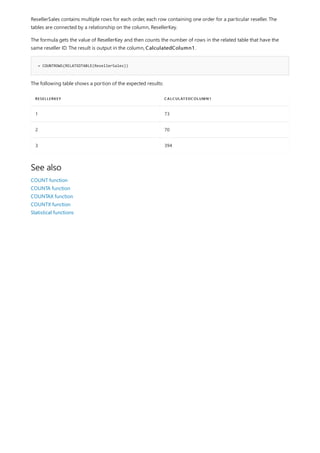
![0000124 20 Counts as 20
0000125 n/a Counts as 0
0000126 Counts as 0
0000126 TRUE Counts as 1
TRANSACTION ID AMOUNT RESULT
= AVERAGEA([Amount])
See also
AVERAGE function
AVERAGEX function
Statistical functions](https://image.slidesharecdn.com/funcoesdax-220812141017-bb6cd4dc/85/Funcoes-DAX-pdf-56-320.jpg)
![AVERAGEX
11/30/2021 • 2 minutes to read
Syntax
AVERAGEX(<table>,<expression>)
Parameters
TERM DEFINITION
table Name of a table, or an expression that specifies the table
over which the aggregation can be performed.
expression An expression with a scalar result, which will be evaluated for
each row of the table in the first argument.
Return value
Remarks
Example
= AVERAGEX(InternetSales, InternetSales[Freight]+ InternetSales[TaxAmt])
See also
Calculates the average (arithmetic mean) of a set of expressions evaluated over a table.
A decimal number.
The AVERAGEX function enables you to evaluate expressions for each row of a table, and then take the
resulting set of values and calculate its arithmetic mean. Therefore, the function takes a table as its first
argument, and an expression as the second argument.
In all other respects, AVERAGEX follows the same rules as AVERAGE. You cannot include non-numeric or
null cells. Both the table and expression arguments are required.
When there are no rows to aggregate, the function returns a blank. When there are rows, but none of
them meet the specified criteria, then the function returns 0.
This function is not supported for use in DirectQuery mode when used in calculated columns or row-
level security (RLS) rules.
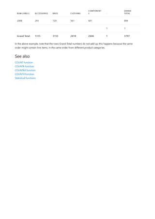
The following example calculates the average freight and tax on each order in the InternetSales table, by first
summing Freight plus TaxAmt in each row, and then averaging those sums.
If you use multiple operations in the expression used as the second argument, you must use parentheses to
control the order of calculations. For more information, see DAX Syntax Reference.](https://image.slidesharecdn.com/funcoesdax-220812141017-bb6cd4dc/85/Funcoes-DAX-pdf-57-320.jpg)

![COUNT
11/30/2021 • 2 minutes to read
Syntax
COUNT(<column>)
Parameters
TERM DEFINITION
column The column that contains the values to be counted.
Return value
Remarks
Example
= COUNT([ShipDate])
See also
The COUNT function counts the number of cells in a column that contain non-blank values.
A whole number.
The only argument allowed to this function is a column. The COUNT function counts rows that contain
the following kinds of values:
Numbers
Dates
Strings
When the function finds no rows to count, it returns a blank.
Blank values are skipped. TRUE/FALSE values are not supported.
If you want to evaluate a column of TRUE/FALSE values, use the COUNTA function.
This function is not supported for use in DirectQuery mode when used in calculated columns or row-
level security (RLS) rules.
For best practices when using COUNT, see Use COUNTROWS instead of COUNT.
The following example shows how to count the number of values in the column, ShipDate.
To count logical values or text, use the COUNTA or COUNTAX functions.
COUNTA function
COUNTAX function](https://image.slidesharecdn.com/funcoesdax-220812141017-bb6cd4dc/85/Funcoes-DAX-pdf-59-320.jpg)

![COUNTA
11/30/2021 • 2 minutes to read
Syntax
COUNTA(<column>)
Parameters
TERM DEFINITION
column The column that contains the values to be counted
Return value
Remarks
Example
= COUNTA('Reseller'[Phone])
See also
The COUNTA function counts the number of cells in a column that are not empty.
A whole number.
When the function does not find any rows to count, the function returns a blank.
This function is not supported for use in DirectQuery mode when used in calculated columns or row-
level security (RLS) rules.
The following example returns all rows in the Reseller table that have any kind of value in the column that
stores phone numbers. Because the table name does not contain any spaces, the quotation marks are optional.
COUNT function
COUNTAX function
COUNTX function
Statistical functions](https://image.slidesharecdn.com/funcoesdax-220812141017-bb6cd4dc/85/Funcoes-DAX-pdf-61-320.jpg)
![COUNTAX
11/30/2021 • 2 minutes to read
Syntax
COUNTAX(<table>,<expression>)
Parameters
TERM DEFINITION
table The table containing the rows for which the expression will
be evaluated.
expression The expression to be evaluated for each row of the table.
Return value
Remarks
Example
= COUNTAX(FILTER('Reseller',[Status]="Active"),[Phone])
See also
The COUNTAX function counts nonblank results when evaluating the result of an expression over a table. That is,
it works just like the COUNTA function, but is used to iterate through the rows in a table and count rows where
the specified expressions results in a non-blank result.
A whole number.
Like the COUNTA function, the COUNTAX function counts cells containing any type of information,
including other expressions. For example, if the column contains an expression that evaluates to an empty
string, the COUNTAX function treats that result as non-blank. Usually the COUNTAX function does not
count empty cells but in this case the cell contains a formula, so it is counted.
Whenever the function finds no rows to aggregate, the function returns a blank.
This function is not supported for use in DirectQuery mode when used in calculated columns or row-
level security (RLS) rules.
The following example counts the number of nonblank rows in the column, Phone, using the table that results
from filtering the Reseller table on [Status] = Active.
COUNT function
COUNTA function
COUNTX function
Statistical functions](https://image.slidesharecdn.com/funcoesdax-220812141017-bb6cd4dc/85/Funcoes-DAX-pdf-62-320.jpg)
![COUNTBLANK
11/30/2021 • 2 minutes to read
Syntax
COUNTBLANK(<column>)
Parameters
TERM DEFINITION
column The column that contains the blank cells to be counted.
Return value
Remarks
Example
= COUNTBLANK(Reseller[BankName])
See also
Counts the number of blank cells in a column.
A whole number. If no rows are found that meet the condition, blanks are returned.
The only argument allowed to this function is a column. You can use columns containing any type of data,
but only blank cells are counted. Cells that have the value zero (0) are not counted, as zero is considered a
numeric value and not a blank.
Whenever there are no rows to aggregate, the function returns a blank. However, if there are rows, but
none of them meet the specified criteria, the function returns 0. Microsoft Excel also returns a zero if no
rows are found that meet the conditions.
In other words, if the COUNTBLANK function finds no blanks, the result will be zero, but if there are no
rows to check, the result will be blank.
This function is not supported for use in DirectQuery mode when used in calculated columns or row-
level security (RLS) rules.
The following example shows how to count the number of rows in the table Reseller that have blank values for
BankName.
To count logical values or text, use the COUNTA or COUNTAX functions.
COUNT function
COUNTA function
COUNTAX function](https://image.slidesharecdn.com/funcoesdax-220812141017-bb6cd4dc/85/Funcoes-DAX-pdf-63-320.jpg)

![COUNTROWS
11/30/2021 • 2 minutes to read
Syntax
COUNTROWS([<table>])
Parameters
TERM DEFINITION
table (Optional) The name of the table that contains the rows to
be counted, or an expression that returns a table. When not
provided, the default value is the home table of the current
expression.
Return value
Remarks
Example 1
= COUNTROWS('Orders')
Example 2
The COUNTROWS function counts the number of rows in the specified table, or in a table defined by an
expression.
A whole number.
This function can be used to count the number of rows in a base table, but more often is used to count
the number of rows that result from filtering a table, or applying context to a table.
Whenever there are no rows to aggregate, the function returns a blank. However, if there are rows, but
none of them meet the specified criteria, the function returns 0. Microsoft Excel also returns a zero if no
rows are found that meet the conditions.
To learn more about best practices when using COUNT and COUNTROWS, see Use COUNTROWS instead
of COUNT in DAX.
This function is not supported for use in DirectQuery mode when used in calculated columns or row-
level security (RLS) rules.
The following example shows how to count the number of rows in the table Orders. The expected result is
52761.
The following example demonstrates how to use COUNTROWS with a row context. In this scenario, there are
two sets of data that are related by order number. The table Reseller contains one row for each reseller; the table](https://image.slidesharecdn.com/funcoesdax-220812141017-bb6cd4dc/85/Funcoes-DAX-pdf-65-320.jpg)
![COUNTX
11/30/2021 • 2 minutes to read
Syntax
COUNTX(<table>,<expression>)
Parameters
TERM DEFINITION
table The table containing the rows to be counted.
expression An expression that returns the set of values that contains
the values you want to count.
Return value
Remarks
Example 1
= COUNTX(Product,[ListPrice])
Example 2
Counts the number of rows that contain a non-blank value or an expression that evaluates to a non-blank value,
when evaluating an expression over a table.
An integer.
The COUNTX function takes two arguments. The first argument must always be a table, or any expression
that returns a table. The second argument is the column or expression that is searched by COUNTX.
The COUNTX function counts only values, dates, or strings. If the function finds no rows to count, it
returns a blank.
If you want to count logical values, use the COUNTAX function.
This function is not supported for use in DirectQuery mode when used in calculated columns or row-
level security (RLS) rules.
The following formula returns a count of all rows in the Product table that have a list price.
The following formula illustrates how to pass a filtered table to COUNTX for the first argument. The formula
uses a filter expression to get only the rows in the Product table that meet the condition, ProductSubCategory =
"Caps", and then counts the rows in the resulting table that have a list price. The FILTER expression applies to the
table Products but uses a value that you look up in the related table, ProductSubCategory.](https://image.slidesharecdn.com/funcoesdax-220812141017-bb6cd4dc/85/Funcoes-DAX-pdf-67-320.jpg)
![= COUNTX(FILTER(Product,RELATED(ProductSubcategory[EnglishProductSubcategoryName])="Caps"),
Product[ListPrice])
See also
COUNT function
COUNTA function
COUNTAX function
Statistical functions](https://image.slidesharecdn.com/funcoesdax-220812141017-bb6cd4dc/85/Funcoes-DAX-pdf-68-320.jpg)
![DISTINCTCOUNT
11/30/2021 • 2 minutes to read
Syntax
DISTINCTCOUNT(<column>)
Parameters
TERM DESCRIPTION
column The column that contains the values to be counted
Return value
Remarks
Example
= DISTINCTCOUNT(ResellerSales_USD[SalesOrderNumber])
ROW LABELS ACCESSORIES BIKES CLOTHING
COMPONENT
S -
GRAND
TOTAL
2005 135 345 242 205 366
2006 356 850 644 702 1015
2007 531 1234 963 1138 1521
Counts the number of distinct values in a column.
The number of distinct values in column.
The only argument allowed to this function is a column. You can use columns containing any type of data.
When the function finds no rows to count, it returns a BLANK, otherwise it returns the count of distinct
values.
DISTINCTCOUNT function includes the BLANK value. To skip the BLANK value, use the
DISTINCTCOUNTNOBLANK function.
This function is not supported for use in DirectQuery mode when used in calculated columns or row-
level security (RLS) rules.
The following example shows how to count the number of distinct sales orders in the column
ResellerSales_USD[SalesOrderNumber].
Using the above measure in a table with calendar year in the side and product category on top returns the
following results:](https://image.slidesharecdn.com/funcoesdax-220812141017-bb6cd4dc/85/Funcoes-DAX-pdf-69-320.jpg)
![DISTINCTCOUNTNOBLANK
11/30/2021 • 2 minutes to read
Syntax
DISTINCTCOUNTNOBLANK (<column>)
Parameters
TERM DESCRIPTION
column The column that contains the values to be counted
Return value
Remarks
Example
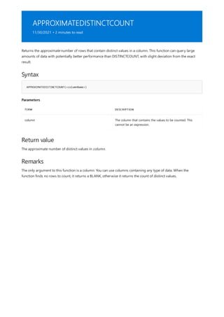
= DISTINCTCOUNT(ResellerSales_USD[SalesOrderNumber])
EVALUATE
ROW(
"DistinctCountNoBlank", DISTINCTCOUNTNOBLANK(DimProduct[EndDate]),
"DistinctCount", DISTINCTCOUNT(DimProduct[EndDate])
)
[DISTINCTCOUNTNOBLANK] [DISTINCTCOUNT]
2 3
See also
Counts the number of distinct values in a column.
The number of distinct values in column.
Unlike DISTINCTCOUNT function, DISTINCTCOUNTNOBLANK does not include the BLANK value.
This function is not supported for use in DirectQuery mode when used in calculated columns or row-
level security (RLS) rules.
The following example shows how to count the number of distinct sales orders in the column
ResellerSales_USD[SalesOrderNumber].
DAX query
DISTINCTCOUNT](https://image.slidesharecdn.com/funcoesdax-220812141017-bb6cd4dc/85/Funcoes-DAX-pdf-71-320.jpg)
![MAX
11/30/2021 • 2 minutes to read
Syntax
MAX(<column>)
MAX(<expression1>, <expression2>)
Parameters
TERM DEFINITION
column The column in which you want to find the largest value.
expression Any DAX expression which returns a single value.
Return value
Remarks
Example 1
= MAX(InternetSales[ExtendedAmount])
Example 2
= Max([TotalSales], [TotalPurchases])
See also
Returns the largest value in a column, or between two scalar expressions.
The largest value.
When comparing two expressions, blank is treated as 0 when comparing. That is, Max(1, Blank() ) returns
1, and Max( -1, Blank() ) returns 0. If both arguments are blank, MAX returns a blank. If either expression
returns a value which is not allowed, MAX returns an error.
TRUE/FALSE values are not supported. If you want to evaluate a column of TRUE/FALSE values, use the
MAXA function.
The following example returns the largest value found in the ExtendedAmount column of the InternetSales table.
The following example returns the largest value between the result of two expressions.](https://image.slidesharecdn.com/funcoesdax-220812141017-bb6cd4dc/85/Funcoes-DAX-pdf-72-320.jpg)

![MAXA
11/30/2021 • 2 minutes to read
Syntax
MAXA(<column>)
Parameters
TERM DEFINITION
column The column in which you want to find the largest value.
Return value
Remarks
Example 1
= MAXA([ResellerMargin])
Example 2
Returns the largest value in a column.
The largest value.
The MAXA function takes as argument a column, and looks for the largest value among the following
types of values:
Numbers
Dates
Logical values, such as TRUE and FALSE. Rows that evaluate to TRUE count as 1; rows that evaluate to
FALSE count as 0 (zero).
Empty cells are ignored. If the column contains no values that can be used, MAXA returns 0 (zero).
If you want to compare text values, use the MAX function.
This function is not supported for use in DirectQuery mode when used in calculated columns or row-
level security (RLS) rules.
The following example returns the greatest value from a calculated column, named ResellerMargin, that
computes the difference between list price and reseller price.
The following example returns the largest value from a column that contains dates and times. Therefore, this
formula gets the most recent transaction date.](https://image.slidesharecdn.com/funcoesdax-220812141017-bb6cd4dc/85/Funcoes-DAX-pdf-74-320.jpg)
![= MAXA([TransactionDate])
See also
MAX function
MAXX function
Statistical functions](https://image.slidesharecdn.com/funcoesdax-220812141017-bb6cd4dc/85/Funcoes-DAX-pdf-75-320.jpg)
![MAXX
11/30/2021 • 2 minutes to read
Syntax
MAXX(<table>,<expression>)
Parameters
TERM DEFINITION
table The table containing the rows for which the expression will
be evaluated.
expression The expression to be evaluated for each row of the table.
Return value
Remarks
Example 1
= MAXX(InternetSales, InternetSales[TaxAmt]+ InternetSales[Freight])
Example 2
Evaluates an expression for each row of a table and returns the largest value.
The largest value.
The table argument to the MAXX function can be a table name, or an expression that evaluates to a table.
The second argument indicates the expression to be evaluated for each row of the table.
Of the values to evaluate, only the following are counted:
Numbers
Texts
Dates
Blank values are skipped. TRUE/FALSE values are not supported.
This function is not supported for use in DirectQuery mode when used in calculated columns or row-
level security (RLS) rules.
The following formula uses an expression as the second argument to calculate the total amount of taxes and
shipping for each order in the table, InternetSales. The expected result is 375.7184.
The following formula first filters the table InternetSales, by using a FILTER expression, to return a subset of
orders for a specific sales region, defined as [SalesTerritory] = 5. The MAXX function then evaluates the
expression used as the second argument for each row of the filtered table, and returns the highest amount for](https://image.slidesharecdn.com/funcoesdax-220812141017-bb6cd4dc/85/Funcoes-DAX-pdf-76-320.jpg)
![= MAXX(FILTER(InternetSales,[SalesTerritoryCode]="5"), InternetSales[TaxAmt]+ InternetSales[Freight])
See also
taxes and shipping for just those orders. The expected result is 250.3724.
MAX function
MAXA function
Statistical functions](https://image.slidesharecdn.com/funcoesdax-220812141017-bb6cd4dc/85/Funcoes-DAX-pdf-77-320.jpg)
![MIN
11/30/2021 • 2 minutes to read
Syntax
MIN(<column>)
MIN(<expression1>, <expression2>)
Parameters
TERM DEFINITION
column The column in which you want to find the smallest value.
expression Any DAX expression which returns a single value.
Return value
Remarks
Example 1
= MIN([ResellerMargin])
Example 2
Returns the smallest value in a column, or between two scalar expressions.
The smallest value.
The MIN function takes a column or two expressions as an argument, and returns the smallest value. The
following types of values in the columns are counted:
Numbers
Texts
Dates
Blanks
When comparing expressions, blank is treated as 0 when comparing. That is, Min(1,Blank() ) returns 0,
and Min( -1, Blank() ) returns -1. If both arguments are blank, MIN returns a blank. If either expression
returns a value which is not allowed, MIN returns an error.
TRUE/FALSE values are not supported. If you want to evaluate a column of TRUE/FALSE values, use the
MINA function.
The following example returns the smallest value from the calculated column, ResellerMargin.](https://image.slidesharecdn.com/funcoesdax-220812141017-bb6cd4dc/85/Funcoes-DAX-pdf-78-320.jpg)
![= MIN([TransactionDate])
Example 3
= Min([TotalSales], [TotalPurchases])
See also
The following example returns the smallest value from a column that contains dates and times, TransactionDate.
This formula therefore returns the date that is earliest.
The following example returns the smallest value from the result of two scalar expressions.
MINA function
MINX function
Statistical functions](https://image.slidesharecdn.com/funcoesdax-220812141017-bb6cd4dc/85/Funcoes-DAX-pdf-79-320.jpg)
![MINA
11/30/2021 • 2 minutes to read
Syntax
MINA(<column>)
Parameters
TERM DEFINITION
column The column for which you want to find the minimum value.
Return value
Remarks
Example 1
= MINA(InternetSales[Freight])
Example 2
= MINA([PostalCode])
See also
Returns the smallest value in a column.
The smallest value.
The MINA function takes as argument a column that contains numbers, and determines the smallest
value as follows:
If the column contains no values, MINA returns 0 (zero).
Rows in the column that evaluates to logical values, such as TRUE and FALSE are treated as 1 if TRUE
and 0 (zero) if FALSE.
Empty cells are ignored.
If you want to compare text values, use the MIN function.
This function is not supported for use in DirectQuery mode when used in calculated columns or row-
level security (RLS) rules.
The following expression returns the minimum freight charge from the table, InternetSales.
The following expression returns the minimum value in the column, PostalCode. Because the data type of the
column is text, the function does not find any values, and the formula returns zero (0).](https://image.slidesharecdn.com/funcoesdax-220812141017-bb6cd4dc/85/Funcoes-DAX-pdf-80-320.jpg)

![MINX
11/30/2021 • 2 minutes to read
Syntax
MINX(<table>, < expression>)
Parameters
TERM DEFINITION
table The table containing the rows for which the expression will
be evaluated.
expression The expression to be evaluated for each row of the table.
Return value
Remarks
Example 1
= MINX( FILTER(InternetSales, [SalesTerritoryKey] = 5),[Freight])
Example 2
= MINX( FILTER(InternetSales, InternetSales[SalesTerritoryKey] = 5), InternetSales[Freight] +
InternetSales[TaxAmt])
Returns the smallest value that results from evaluating an expression for each row of a table.
A smallest value.
The MINX function takes as its first argument a table, or an expression that returns a table. The second
argument contains the expression that is evaluated for each row of the table.
Blank values are skipped. TRUE/FALSE values are not supported.
This function is not supported for use in DirectQuery mode when used in calculated columns or row-
level security (RLS) rules.
The following example filters the table, InternetSales, and returns only rows for a specific sales territory. The
formula then finds the minimum value in the column, Freight.
The following example uses the same filtered table as in the previous example, but instead of merely looking up
values in the column for each row of the filtered table, the function calculates the sum of two columns, Freight
and TaxAmt, and returns the smallest value resulting from that calculation.](https://image.slidesharecdn.com/funcoesdax-220812141017-bb6cd4dc/85/Funcoes-DAX-pdf-82-320.jpg)
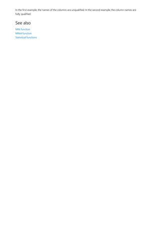
![PRODUCT
11/30/2021 • 2 minutes to read
Syntax
PRODUCT(<column>)
Parameters
TERM DEFINITION
column The column that contains the numbers for which the
product is to be computed.
Return value
Remarks
Example
= PRODUCT( Annuity[AdjustedRates] )
See also
Returns the product of the numbers in a column.
A decimal number.
To return the product of an expression evaluated for each row in a table, use PRODUCTX function.
Only the numbers in the column are counted. Blanks, logical values, and text are ignored. For example,
PRODUCT( Table[Column] ) is equivalent to PRODUCTX( Table, Table[Column] ) .
This function is not supported for use in DirectQuery mode when used in calculated columns or row-
level security (RLS) rules.
The following computes the product of the AdjustedRates column in an Annuity table:
PRODUCTX](https://image.slidesharecdn.com/funcoesdax-220812141017-bb6cd4dc/85/Funcoes-DAX-pdf-84-320.jpg)
![PRODUCTX
11/30/2021 • 2 minutes to read
Syntax
PRODUCTX(<table>, <expression>)
Parameters
TERM DEFINITION
table The table containing the rows for which the expression will
be evaluated.
expression The expression to be evaluated for each row of the table.
Return value
Remarks
Example
= [PresentValue] * PRODUCTX( AnnuityPeriods, 1+[FixedInterestRate] )
See also
Returns the product of an expression evaluated for each row in a table.
A decimal number.
To return the product of the numbers in a column, use PRODUCT.
The PRODUCTX function takes as its first argument a table, or an expression that returns a table. The
second argument is a column that contains the numbers for which you want to compute the product, or
an expression that evaluates to a column.
Only the numbers in the column are counted. Blanks, logical values, and text are ignored.
This function is not supported for use in DirectQuery mode when used in calculated columns or row-
level security (RLS) rules.
The following computes the future value of an investment:
PRODUCT](https://image.slidesharecdn.com/funcoesdax-220812141017-bb6cd4dc/85/Funcoes-DAX-pdf-85-320.jpg)
![SUM
11/30/2021 • 2 minutes to read
Syntax
SUM(<column>)
Parameters
TERM DEFINITION
column The column that contains the numbers to sum.
Return value
Remarks
Example
= SUM(Sales[Amt])
See also
Adds all the numbers in a column.
A decimal number.
If you want to filter the values that you are summing, you can use the SUMX function and specify an expression
to sum over.
The following example adds all the numbers that are contained in the column, Amt, from the table, Sales.
SUMX](https://image.slidesharecdn.com/funcoesdax-220812141017-bb6cd4dc/85/Funcoes-DAX-pdf-86-320.jpg)
![SUMX
11/30/2021 • 2 minutes to read
Syntax
SUMX(<table>, <expression>)
Parameters
TERM DEFINITION
table The table containing the rows for which the expression will
be evaluated.
expression The expression to be evaluated for each row of the table.
Return value
Remarks
Example
= SUMX(FILTER(InternetSales, InternetSales[SalesTerritoryID]=5),[Freight])
See also
Returns the sum of an expression evaluated for each row in a table.
A decimal number.
The SUMX function takes as its first argument a table, or an expression that returns a table. The second
argument is a column that contains the numbers you want to sum, or an expression that evaluates to a
column.
Only the numbers in the column are counted. Blanks, logical values, and text are ignored.
For more complex examples of SUMX in formulas, see ALL and CALCULATETABLE.
This function is not supported for use in DirectQuery mode when used in calculated columns or row-
level security (RLS) rules.
The following example first filters the table, InternetSales, on the expression, ShippingTerritoryID = 5 , and then
returns the sum of all values in the column, Freight. In other words, the expression returns the sum of freight
charges for only the specified sales area.
If you do not need to filter the column, use the SUM function. The SUM function is similar to the Excel function
of the same name, except that it takes a column as a reference.
SUM](https://image.slidesharecdn.com/funcoesdax-220812141017-bb6cd4dc/85/Funcoes-DAX-pdf-87-320.jpg)

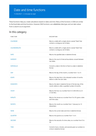
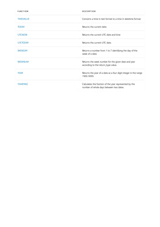
![CALENDAR
11/30/2021 • 2 minutes to read
Syntax
CALENDAR(<start_date>, <end_date>)
Parameters
TERM DEFINITION
start_date Any DAX expression that returns a datetime value.
end_date Any DAX expression that returns a datetime value.
Return value
Remarks
Examples
= CALENDAR (DATE (2005, 1, 1), DATE (2015, 12, 31))
= CALENDAR (MINX (Sales, [Date]), MAXX (Forecast, [Date]))
Returns a table with a single column named "Date" that contains a contiguous set of dates. The range of dates is
from the specified start date to the specified end date, inclusive of those two dates.
Returns a table with a single column named "Date" containing a contiguous set of dates. The range of dates is
from the specified start date to the specified end date, inclusive of those two dates.
An error is returned if start_date is greater than end_date.
This function is not supported for use in DirectQuery mode when used in calculated columns or row-
level security (RLS) rules.
The following formula returns a table with dates between January 1st, 2005 and December 31st, 2015.
For a data model which includes actual sales data and future sales forecasts. The following expression returns
the date table covering the range of dates in these two tables.](https://image.slidesharecdn.com/funcoesdax-220812141017-bb6cd4dc/85/Funcoes-DAX-pdf-91-320.jpg)
![CALENDARAUTO
11/30/2021 • 2 minutes to read
Syntax
CALENDARAUTO([fiscal_year_end_month])
Parameters
TERM DEFINITION
fiscal_year_end_month Any DAX expression that returns an integer from 1 to 12. If
omitted, defaults to the value specified in the calendar table
template for the current user, if present; otherwise, defaults
to 12.
Return value
Remarks
Example
Returns a table with a single column named "Date" that contains a contiguous set of dates. The range of dates is
calculated automatically based on data in the model.
Returns a table with a single column named "Date" that contains a contiguous set of dates. The range of dates is
calculated automatically based on data in the model.
The date range is calculated as follows:
The earliest date in the model which is not in a calculated column or calculated table is taken as the
MinDate.
The latest date in the model which is not in a calculated column or calculated table is taken as the
MaxDate.
The date range returned is dates between the beginning of the fiscal year associated with MinDate and
the end of the fiscal year associated with MaxDate.
An error is returned if the model does not contain any datetime values which are not in calculated
columns or calculated tables.
This function is not supported for use in DirectQuery mode when used in calculated columns or row-
level security (RLS) rules.
In this example, the MinDate and MaxDate in the data model are July 1, 2010 and June 30, 2011.
CALENDARAUTO() will return all dates between January 1, 2010 and December 31, 2011.
CALENDARAUTO(3) will return all dates between March 1, 2010 and March 31, 2012.](https://image.slidesharecdn.com/funcoesdax-220812141017-bb6cd4dc/85/Funcoes-DAX-pdf-92-320.jpg)
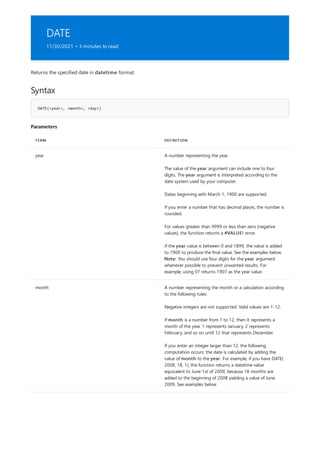
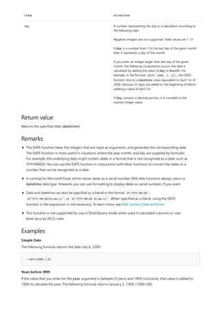
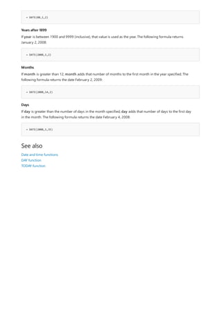
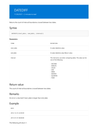
![DATEDIFF(MIN( Calendar[Date] ), MAX( Calendar[Date]), SECOND )
DATEDIFF(MIN( Calendar[Date] ), MAX( Calendar[Date]), MINUTE )
DATEDIFF(MIN( Calendar[Date] ), MAX( Calendar[Date]), HOUR )
DATEDIFF(MIN( Calendar[Date] ), MAX( Calendar[Date]), DAY )
DATEDIFF(MIN( Calendar[Date] ), MAX( Calendar[Date]), WEEK )
DATEDIFF(MIN( Calendar[Date] ), MAX( Calendar[Date]), MONTH )
DATEDIFF(MIN( Calendar[Date] ), MAX( Calendar[Date]), QUARTER )
DATEDIFF(MIN( Calendar[Date] ), MAX( Calendar[Date]), YEAR )](https://image.slidesharecdn.com/funcoesdax-220812141017-bb6cd4dc/85/Funcoes-DAX-pdf-97-320.jpg)
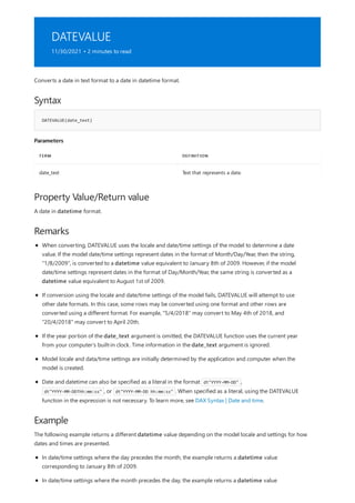
![DAY
11/30/2021 • 2 minutes to read
Syntax
DAY(<date>)
Parameters
TERM DEFINITION
date A date in datetime format, or a text representation of a
date.
Return value
Remarks
Example: Getting the day from a date column
= DAY([Birthdate])
Example - Getting the day from a string date
Returns the day of the month, a number from 1 to 31.
An integer number indicating the day of the month.
The DAY function takes as an argument the date of the day you are trying to find. Dates can be provided
to the function by using another date function, by using an expression that returns a date, or by typing a
date in a datetime format. You can also type a date in one of the accepted string formats for dates.
Values returned by the YEAR, MONTH and DAY functions will be Gregorian values regardless of the
display format for the supplied date value. For example, if the display format of the supplied date is Hijri,
the returned values for the YEAR, MONTH and DAY functions will be values associated with the equivalent
Gregorian date.
When the date argument is a text representation of the date, the day function uses the locale and
date/time settings of the client computer to understand the text value in order to perform the conversion.
If the current date/time settings represent dates in the format of Month/Day/Year, then the string,
"1/8/2009", is interpreted as a datetime value equivalent to January 8th of 2009, and the function
returns 8. However, if the current date/time settings represent dates in the format of Day/Month/Year, the
same string would be interpreted as a datetime value equivalent to August 1st of 2009, and the function
returns 1.
The following formula returns the day from the date in the column, [Birthdate].
The following formulas return the day, 4, using dates that have been supplied as strings in an accepted text
format.](https://image.slidesharecdn.com/funcoesdax-220812141017-bb6cd4dc/85/Funcoes-DAX-pdf-100-320.jpg)
![= DAY("3-4-1007")
= DAY("March 4 2007")
Example - Using a day value as a condition
= IF( DAY([SalesDate])=10,"promotion","")
See also
The following expression returns the day that each sales order was placed, and flags the row as a promotional
sale item if the order was placed on the 10th of the month.
Date and time functions
TODAY function
DATE function](https://image.slidesharecdn.com/funcoesdax-220812141017-bb6cd4dc/85/Funcoes-DAX-pdf-101-320.jpg)
![= EDATE([TransactionDate],3)
See also
The following example returns the date three months after the order date, which is stored in the column
[TransactionDate].
EOMONTH function
Date and time functions](https://image.slidesharecdn.com/funcoesdax-220812141017-bb6cd4dc/85/Funcoes-DAX-pdf-103-320.jpg)
![HOUR
11/30/2021 • 2 minutes to read
Syntax
HOUR(<datetime>)
Parameters
TERM DEFINITION
datetime A datetime value, such as 16:48:00 or 4:48 PM.
Return value
Remarks
Example 1
= HOUR('Orders'[TransactionTime])
Example 2
= HOUR("March 3, 2008 3:00 PM")
See also
Returns the hour as a number from 0 (12:00 A.M.) to 23 (11:00 P.M.).
An integer number from 0 to 23.
The HOUR function takes as argument the time that contains the hour you want to find. You can supply
the time by using a date/time function, an expression that returns a datetime, or by typing the value
directly in one of the accepted time formats. Times can also be entered as any accepted text
representation of a time.
When the datetime argument is a text representation of the date and time, the function uses the locale
and date/time settings of the client computer to understand the text value in order to perform the
conversion. Most locales use the colon (:) as the time separator and any input text using colons as time
separators will parse correctly. Review your locale settings to understand your results.
The following example returns the hour from the TransactionTime column of a table named Orders.
The following example returns 15, meaning the hour corresponding to 3 PM in a 24-hour clock. The text value is
automatically parsed and converted to a date/time value.
Date and time functions](https://image.slidesharecdn.com/funcoesdax-220812141017-bb6cd4dc/85/Funcoes-DAX-pdf-106-320.jpg)

![MINUTE
11/30/2021 • 2 minutes to read
Syntax
MINUTE(<datetime>)
Parameters
TERM DEFINITION
datetime A datetime value or text in an accepted time format, such
as 16:48:00 or 4:48 PM.
Return value
Remarks
Example 1
= MINUTE(Orders[TransactionTime])
Example 2
= MINUTE("March 23, 2008 1:45 PM")
See also
Returns the minute as a number from 0 to 59, given a date and time value.
An integer number from 0 to 59.
In contrast to Microsoft Excel, which stores dates and times in a serial numeric format, DAX uses a
datetime data type for dates and times. You can provide the datetime value to the MINUTE function by
referencing a column that stores dates and times, by using a date/time function, or by using an
expression that returns a date and time.
When the datetime argument is a text representation of the date and time, the function uses the locale
and date/time settings of the client computer to understand the text value in order to perform the
conversion. Most locales use the colon (:) as the time separator and any input text using colons as time
separators will parse correctly. Verify your locale settings to understand your results.
The following example returns the minute from the value stored in the TransactionTime column of the Orders
table.
The following example returns 45, which is the number of minutes in the time 1:45 PM.](https://image.slidesharecdn.com/funcoesdax-220812141017-bb6cd4dc/85/Funcoes-DAX-pdf-108-320.jpg)

![Example 2
= MONTH(Orders[TransactionDate])
See also
The following expression returns the month from the date in the TransactionDate column of the Orders table.
Date and time functions
HOUR function
MINUTE function
YEAR function
SECOND function](https://image.slidesharecdn.com/funcoesdax-220812141017-bb6cd4dc/85/Funcoes-DAX-pdf-111-320.jpg)
![QUARTER
11/30/2021 • 2 minutes to read
Syntax
QUARTER(<date>)
Parameters
TERM DEFINITION
date A date.
Return value
Remarks
Example 1
EVALUATE { QUARTER(DATE(2019, 2, 1)), QUARTER(DATE(2018, 12, 31)) }
[VALUE]
1
4
Example 2
Returns the quarter as a number from 1 (January – March) to 4 (October – December).
An integer number from 1 to 4.
If the input value is BLANK, the output value is also BLANK.
The following DAX query:
Returns:
The following DAX query:](https://image.slidesharecdn.com/funcoesdax-220812141017-bb6cd4dc/85/Funcoes-DAX-pdf-113-320.jpg)
![EVALUATE
ADDCOLUMNS(
FILTER(
VALUES(
FactInternetSales[OrderDate]),
[OrderDate] >= DATE(2008, 3, 31) && [OrderDate] <= DATE(2008, 4, 1)
),
"Quarter", QUARTER([OrderDate])
)
FACTINTERNETSALES[ORDERDATE] [QUARTER]
3/31/2008 1
4/1/2008 2
See also
Returns:
YEAR
MONTH
DAY](https://image.slidesharecdn.com/funcoesdax-220812141017-bb6cd4dc/85/Funcoes-DAX-pdf-114-320.jpg)
![SECOND
11/30/2021 • 2 minutes to read
Syntax
SECOND(<time>)
Parameters
TERM DEFINITION
time A time in datetime format, such as 16:48:23 or 4:48:47 PM.
Return value
Remarks
Example 1
= SECOND('Orders'[TransactionTime])
Returns the seconds of a time value, as a number from 0 to 59.
An integer number from 0 to 59.
In contrast to Microsoft Excel, which stores dates and times as serial numbers, DAX uses a datetime
format when working with dates and times. If the source data is not in this format, DAX implicitly
converts the data. You can use formatting to display the dates and times as a serial number of you need
to.
The date/time value that you supply as an argument to the SECOND function can be entered as a text
string within quotation marks (for example, "6:45 PM"). You can also provide a time value as the result of
another expression, or as a reference to a column that contains times.
If you provide a numeric value of another data type, such as 13.60, the value is interpreted as a serial
number and is represented as a datetime data type before extracting the value for seconds. To make it
easier to understand your results, you might want to represent such numbers as dates before using them
in the SECOND function. For example, if you use SECOND with a column that contains a numeric value
such as, 25.56, the formula returns 24. That is because, when formatted as a date, the value 25.56 is
equivalent to January 25, 1900, 1:26:24 PM.
When the time argument is a text representation of a date and time, the function uses the locale and
date/time settings of the client computer to understand the text value in order to perform the conversion.
Most locales use the colon (:) as the time separator and any input text using colons as time separators will
parse correctly. Review your locale settings to understand your results.
The following formula returns the number of seconds in the time contained in the TransactionTime column of
a table named Orders.](https://image.slidesharecdn.com/funcoesdax-220812141017-bb6cd4dc/85/Funcoes-DAX-pdf-115-320.jpg)
![Example 1
= TIME(27,0,0)
= TIME(3,0,0)
Example 2
= TIME(0,750,0)
= TIME(12,30,0)
Example 3
= TIME([intHours],[intMinutes],[intSeconds])
See also
time values in a datetime format. Numbers in other formats are implicitly converted when you use a
date/time value in a DAX function. If you need to use serial numbers, you can use formatting to change
the way that the numbers are displayed.
Time values are a portion of a date value, and in the serial number system are represented by a decimal
number. Therefore, the datetime value 12:00 PM is equivalent to 0.5, because it is half of a day.
You can supply the arguments to the TIME function as values that you type directly, as the result of
another expression, or by a reference to a column that contains a numeric value.
Date and datetime can also be specified as a literal in the format dt"YYYY-MM-DD" ,
dt"YYYY-MM-DDThh:mm:ss" , or dt"YYYY-MM-DD hh:mm:ss" . When specified as a literal, using the TIME
function in the expression is not necessary. To learn more, see DAX Syntax | Date and time.
This function is not supported for use in DirectQuery mode when used in calculated columns or row-
level security (RLS) rules.
The following examples both return the time, 3:00 AM:
The following examples both return the time, 12:30 PM:
The following example creates a time based on the values in the columns, intHours , intMinutes , intSeconds :
DATE
Date and time functions](https://image.slidesharecdn.com/funcoesdax-220812141017-bb6cd4dc/85/Funcoes-DAX-pdf-118-320.jpg)
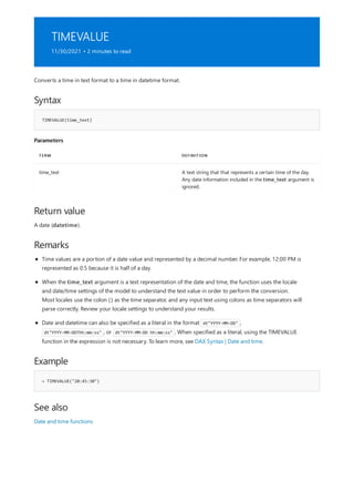
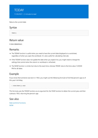
![UTCNOW
11/30/2021 • 2 minutes to read
Syntax
UTCNOW()
Return value
Remarks
Example
EVALUATE { FORMAT(UTCNOW(), "General Date") }
[VALUE]
2/2/2018 4:48:08 AM
See also
Returns the current UTC date and time.
A (datetime).
The result of the UTCNOW function changes only when the formula is refreshed. It is not continuously updated.
The following:
Returns:
NOW function
UTCTODAY function](https://image.slidesharecdn.com/funcoesdax-220812141017-bb6cd4dc/85/Funcoes-DAX-pdf-121-320.jpg)
![UTCTODAY
11/30/2021 • 2 minutes to read
Syntax
UTCTODAY()
Return value
Remarks
Example
EVALUATE { FORMAT(UTCTODAY(), "General Date") }
[VALUE]
2/2/2018
See also
Returns the current UTC date.
A date.
UTCTODAY returns the time value 12:00:00 PM for all dates.
The UTCNOW function is similar but returns the exact time and date.
The following:
Returns:
NOW function
UTCNOW function](https://image.slidesharecdn.com/funcoesdax-220812141017-bb6cd4dc/85/Funcoes-DAX-pdf-122-320.jpg)
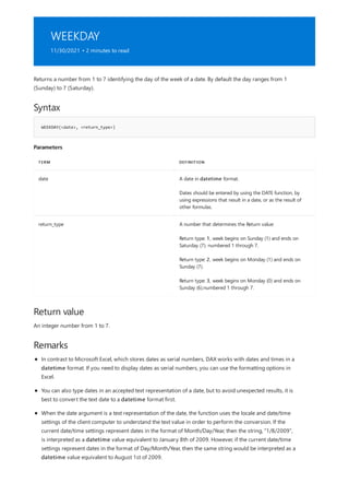
![Example
= WEEKDAY([HireDate]+1)
See also
The following example gets the date from the [HireDate] column, adds 1, and displays the weekday
corresponding to that date. Because the return_type argument has been omitted, the default format is used, in
which 1 is Sunday and 7 is Saturday. If the result is 4, the day would be Wednesday.
Date and time functions
WEEKNUM function
YEARFRAC function](https://image.slidesharecdn.com/funcoesdax-220812141017-bb6cd4dc/85/Funcoes-DAX-pdf-124-320.jpg)
![WEEKNUM
11/30/2021 • 2 minutes to read
Syntax
WEEKNUM(<date>[, <return_type>])
Parameters
TERM DEFINITION
date The date in datetime format.
return_type (Optional) A number that determines on which day the week
begins. Default is 1. See Remarks.
Return value
Remarks
Returns the week number for the given date according to the return_type value. The week number indicates
where the week falls numerically within a year.
There are two systems used for this function:
System 1 - The week containing January 1 is the first week of the year and is numbered week 1.
System 2 - The week containing the first Thursday of the year is the first week of the year and is numbered
as week 1. This system is the methodology specified in ISO 8601, which is commonly known as the European
week numbering system.
An integer number.
RETURN_TYPE WEEK BEGINS ON SYSTEM
1 or omitted Sunday 1
2 Monday 1
By default, the WEEKNUM function uses a calendar convention in which the week containing January 1 is
considered to be the first week of the year. However, the ISO 8601 calendar standard, widely used in
Europe, defines the first week as the one with the majority of days (four or more) falling in the new year.
This means that if return_type is any valid value other than 21, for any years in which there are three
days or less in the first week of January, the WEEKNUM function returns week numbers that are different
from the ISO 8601 definition.
For return_type, except for 21, the following valid values may not be supported by some DirectQuery
data sources:](https://image.slidesharecdn.com/funcoesdax-220812141017-bb6cd4dc/85/Funcoes-DAX-pdf-125-320.jpg)
![Example 1
= WEEKNUM("Feb 14, 2010", 2)
Example 2
= WEEKNUM('Employees'[HireDate])
See also
11 Monday 1
12 Tuesday 1
13 Wednesday 1
14 Thursday 1
15 Friday 1
16 Saturday 1
17 Sunday 1
21 Monday 2
RETURN_TYPE WEEK BEGINS ON SYSTEM
The following example returns the week number for February 14, 2010. This calculation assumes weeks begin
on Monday.
The following example returns the week number of the date stored in the column, HireDate, from the table,
Employees. This calculation assumes weeks begin on Sunday.
YEARFRAC function
WEEKDAY function](https://image.slidesharecdn.com/funcoesdax-220812141017-bb6cd4dc/85/Funcoes-DAX-pdf-126-320.jpg)
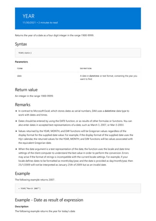
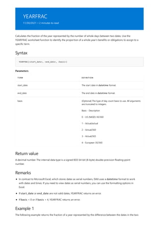
![= YEARFRAC(Orders[TransactionDate],Orders[ShippingDate])
Example 2
= YEARFRAC("Jan 1 2007","Mar 1 2007")
See also
columns, TransactionDate and ShippingDate :
The following example returns the fraction of a year represented by the difference between the dates, January 1
and March 1:
Use four-digit years whenever possible, to avoid getting unexpected results. When the year is truncated, the
current year is assumed. When the date is or omitted, the first date of the month is assumed.
The second argument, basis, has also been omitted. Therefore, the year fraction is calculated according to the
US (NASD) 30/360 standard.
Date and time functions
WEEKNUM function
YEARFRAC function
WEEKDAY function](https://image.slidesharecdn.com/funcoesdax-220812141017-bb6cd4dc/85/Funcoes-DAX-pdf-130-320.jpg)


![ALL
11/30/2021 • 7 minutes to read
Syntax
ALL( [<table> | <column>[, <column>[, <column>[,…]]]] )
Parameters
TERM DEFINITION
table The table that you want to clear filters on.
column The column that you want to clear filters on.
Return value
Remarks
Returns all the rows in a table, or all the values in a column, ignoring any filters that might have been applied.
This function is useful for clearing filters and creating calculations on all the rows in a table.
The argument to the ALL function must be either a reference to a base table or a reference to a base column. You
cannot use table expressions or column expressions with the ALL function.
The table or column with filters removed.
FUNCTION AND USAGE DESCRIPTION
ALL() Removes all filters everywhere. ALL() can only be used to
clear filters but not to return a table.
This function is not used by itself, but serves as an intermediate function that can be used to change the
set of results over which some other calculation is performed.
The normal behavior for DAX expressions containing the ALL() function is that any filters applied will be
ignored. However, there are some scenarios where this is not the case because of auto-exist, a DAX
technology that optimizes filtering in order to reduce the amount of processing required for certain DAX
queries. An example where auto-exist and ALL() provide unexpected results is when filtering on two or
more columns of the same table (like when using slicers), and there is a measure on that same table that
uses ALL(). In this case, auto-exist will merge the multiple filters into one and will only filter on existing
combinations of values. Because of this merge, the measure will be calculated on the existing
combinations of values and the result will be based on filtered values instead of all values as expected. To
learn more about auto-exist and its effect on calculations, see Microsoft MVP Alberto Ferrari's
Understanding DAX Auto-Exist article on sql.bi.com.
The following table describes how you can use the ALL and ALLEXCEPT functions in different scenarios.](https://image.slidesharecdn.com/funcoesdax-220812141017-bb6cd4dc/85/Funcoes-DAX-pdf-133-320.jpg)
![Example 1
ROW LABELS ACCESSORIES BIKES CLOTHING COMPONENTS GRAND TOTAL
2005 0.02% 9.10% 0.04% 0.75% 9.91%
2006 0.11% 24.71% 0.60% 4.48% 29.90%
2007 0.36% 31.71% 1.07% 6.79% 39.93%
2008 0.20% 16.95% 0.48% 2.63% 20.26%
Grand Total 0.70% 82.47% 2.18% 14.65% 100.00%
ALL(Table) Removes all filters from the specified table. In effect,
ALL(Table) returns all of the values in the table, removing
any filters from the context that otherwise might have
been applied. This function is useful when you are
working with many levels of grouping, and want to
create a calculation that creates a ratio of an aggregated
value to the total value. The first example demonstrates
this scenario.
ALL (Column[, Column[, …]]) Removes all filters from the specified columns in the
table; all other filters on other columns in the table still
apply. All column arguments must come from the same
table. The ALL(Column) variant is useful when you want
to remove the context filters for one or more specific
columns and to keep all other context filters. The second
and third examples demonstrate this scenario.
ALLEXCEPT(Table, Column1 [,Column2]...) Removes all context filters in the table except filters that
are applied to the specified columns. This is a convenient
shortcut for situations in which you want to remove the
filters on many, but not all, columns in a table.
FUNCTION AND USAGE DESCRIPTION
This function is not supported for use in DirectQuery mode when used in calculated columns or row-
level security (RLS) rules.
Calculate ratio of Category Sales to Total Sales
Assume that you want to find the amount of sales for the current cell, in your PivotTable, divided by the total
sales for all resellers. To ensure that the denominator is the same regardless of how the PivotTable user might be
filtering or grouping the data, you define a formula that uses ALL to create the correct grand total.
The following table shows the results when a new measure, All Reseller Sales Ratio, is created using the
formula shown in the code section. To see how this works, add the field, CalendarYear, to the Row Labels area
of the PivotTable, and add the field, ProductCategoryName, to the Column Labels area. Then, drag the
measure, All Reseller Sales Ratio, to the Values area of the Pivot Table. To view the results as percentages,
use the formatting features of Excel to apply a percentage number formatting to the cells that contains the
measure.
Formula](https://image.slidesharecdn.com/funcoesdax-220812141017-bb6cd4dc/85/Funcoes-DAX-pdf-134-320.jpg)
![= SUMX(ResellerSales_USD, ResellerSales_USD[SalesAmount_USD])/SUMX(ALL(ResellerSales_USD),
ResellerSales_USD[SalesAmount_USD])
Example 2
ROW LABELS ACCESSORIES BIKES CLOTHING COMPONENTS GRAND TOTAL
2005 3.48% 11.03% 1.91% 5.12% 9.91%
2006 16.21% 29.96% 27.29% 30.59% 29.90%
2007 51.62% 38.45% 48.86% 46.36% 39.93%
2008 28.69% 20.56% 21.95% 17.92% 20.26%
Grand Total 100.00% 100.00% 100.00% 100.00% 100.00%
= SUMX(ResellerSales_USD, ResellerSales_USD[SalesAmount_USD])/CALCULATE( SUM(
ResellerSales_USD[SalesAmount_USD]), ALL(DateTime[CalendarYear]))
The formula is constructed as follows:
1. The numerator, SUMX(ResellerSales_USD, ResellerSales_USD[SalesAmount_USD]) , is the sum of the values in
ResellerSales_USD[SalesAmount_USD] for the current cell in the PivotTable, with context filters applied on
CalendarYear and ProductCategoryName.
2. For the denominator, you start by specifying a table, ResellerSales_USD, and use the ALL function to
remove all context filters on the table.
3. You then use the SUMX function to sum the values in the ResellerSales_USD[SalesAmount_USD] column.
In other words, you get the sum of ResellerSales_USD[SalesAmount_USD] for all resellers sales.
Calculate Ratio of Product Sales to Total Sales Through Current Year
Assume that you want to create a table showing the percentage of sales compared over the years for each
product category (ProductCategoryName). To obtain the percentage for each year over each value of
ProductCategoryName, you need to divide the sum of sales for that particular year and product category by the
sum of sales for the same product category over all years. In other words, you want to keep the filter on
ProductCategoryName but remove the filter on the year when calculating the denominator of the percentage.
The following table shows the results when a new measure, Reseller Sales Year, is created using the formula
shown in the code section. To see how this works, add the field, CalendarYear, to the Row Labels area of a
PivotTable, and add the field, ProductCategoryName, to the Column Labels area. To view the results as
percentages, use Excel's formatting features to apply a percentage number format to the cells containing the
measure, Reseller Sales Year.
Formula
The formula is constructed as follows:
1. The numerator, SUMX(ResellerSales_USD, ResellerSales_USD[SalesAmount_USD]) , is the sum of the values in
ResellerSales_USD[SalesAmount_USD] for the current cell in the pivot table, with context filters applied
on the columns CalendarYear and ProductCategoryName.
2. For the denominator, you remove the existing filter on CalendarYear by using the ALL(Column) function.](https://image.slidesharecdn.com/funcoesdax-220812141017-bb6cd4dc/85/Funcoes-DAX-pdf-135-320.jpg)
![Example 3
ROW LABELS ACCESSORIES BIKES CLOTHING COMPONENTS GRAND TOTAL
2005 0.25% 91.76% 0.42% 7.57% 100.00%
2006 0.38% 82.64% 1.99% 14.99% 100.00%
2007 0.90% 79.42% 2.67% 17.01% 100.00%
2008 0.99% 83.69% 2.37% 12.96% 100.00%
Grand Total 0.70% 82.47% 2.18% 14.65% 100.00%
= SUMX(ResellerSales_USD, ResellerSales_USD[SalesAmount_USD])/CALCULATE( SUM(
ResellerSales_USD[SalesAmount_USD]), ALL(ProductCategory[ProductCategoryName]))
See also
This calculates the sum over the remaining rows on the ResellerSales_USD table, after applying the
existing context filters from the column labels. The net effect is that for the denominator the sum is
calculated over the selected ProductCategoryName (the implied context filter) and for all values in Year.
Calculate Contribution of Product Categories to Total Sales Per Year
Assume that you want to create a table that shows the percentage of sales for each product category, on a year-
by-year basis. To obtain the percentage for each product category in a particular year, you need to calculate the
sum of sales for that particular product category (ProductCategoryName) in year n, and then divide the
resulting value by the sum of sales for the year n over all product categories. In other words, you want to keep
the filter on year but remove the filter on ProductCategoryName when calculating the denominator of the
percentage.
The following table shows the results when a new measure, Reseller Sales CategoryName, is created using
the formula shown in the code section. To see how this works, add the field, CalendarYear to the Row Labels
area of the PivotTable, and add the field, ProductCategoryName, to the Column Labels area. Then add the new
measure to the Values area of the PivotTable. To view the results as percentages, use Excel's formatting features
to apply a percentage number format to the cells that contain the new measure, Reseller Sales
CategoryName.
Formula
The formula is constructed as follows:
1. The numerator, SUMX(ResellerSales_USD, ResellerSales_USD[SalesAmount_USD]) , is the sum of the values in
ResellerSales_USD[SalesAmount_USD] for the current cell in the PivotTable, with context filters applied on
the fields, CalendarYear and ProductCategoryName.
2. For the denominator, you use the function, ALL(Column), to remove the filter on ProductCategoryName
and calculate the sum over the remaining rows on the ResellerSales_USD table, after applying the existing
context filters from the row labels. The net effect is that, for the denominator, the sum is calculated over
the selected Year (the implied context filter) and for all values of ProductCategoryName.
Filter functions
ALL function](https://image.slidesharecdn.com/funcoesdax-220812141017-bb6cd4dc/85/Funcoes-DAX-pdf-136-320.jpg)

![ALLCROSSFILTERED
11/30/2021 • 2 minutes to read
Syntax
ALLCROSSFILTERED(<table>)
Parameters
TERM DEFINITION
table The table that you want to clear filters on.
Return value
Remarks
Example
DEFINE
MEASURE FactInternetSales[TotalQuantity1] =
CALCULATE(SUM(FactInternetSales[OrderQuantity]), ALLCROSSFILTERED(FactInternetSales))
MEASURE FactInternetSales[TotalQuantity2] =
CALCULATE(SUM(FactInternetSales[OrderQuantity]), ALL(FactInternetSales))
EVALUATE
SUMMARIZECOLUMNS(DimSalesReason[SalesReasonName],
"TotalQuantity1", [TotalQuantity1],
"TotalQuantity2", [TotalQuantity2])
ORDER BY DimSalesReason[SalesReasonName]
DIMSALESREASON[SALESREASONNAM
E] [TOTALQUANTITY1] [TOTALQUANTITY2]
Demo Event 60398
Magazine Advertisement 60398
Manufacturer 60398 1818
Clear all filters which are applied to a table.
N/A. See remarks.
ALLCROSSFILTERED can only be used to clear filters but not to return a table.
This function is not supported for use in DirectQuery mode when used in calculated columns or row-
level security (RLS) rules.
Returns,](https://image.slidesharecdn.com/funcoesdax-220812141017-bb6cd4dc/85/Funcoes-DAX-pdf-138-320.jpg)
![On Promotion 60398 7390
Other 60398 3653
Price 60398 47733
Quality 60398 1551
Review 60398 1640
Sponsorship 60398
Television Advertisement 60398 730
DIMSALESREASON[SALESREASONNAM
E] [TOTALQUANTITY1] [TOTALQUANTITY2]
NOTE
There is a direct or indirect many-to-many relationship between FactInternetSales table and DimSalesReason table.](https://image.slidesharecdn.com/funcoesdax-220812141017-bb6cd4dc/85/Funcoes-DAX-pdf-139-320.jpg)
![ALLEXCEPT
11/30/2021 • 2 minutes to read
Syntax
ALLEXCEPT(<table>,<column>[,<column>[,…]])
Parameters
TERM DEFINITION
table The table over which all context filters are removed, except
filters on those columns that are specified in subsequent
arguments.
column The column for which context filters must be preserved.
Return value
Remarks
Removes all context filters in the table except filters that have been applied to the specified columns.
The first argument to the ALLEXCEPT function must be a reference to a base table. All subsequent arguments
must be references to base columns. You cannot use table expressions or column expressions with the
ALLEXCEPT function.
A table with all filters removed except for the filters on the specified columns.
FUNCTION AND USAGE DESCRIPTION
ALL(Table) Removes all filters from the specified table. In effect,
ALL(Table) returns all of the values in the table, removing
any filters from the context that otherwise might have
been applied. This function is useful when you are
working with many levels of grouping, and want to
create a calculation that creates a ratio of an aggregated
value to the total value.
ALL (Column[, Column[, …]]) Removes all filters from the specified columns in the
table; all other filters on other columns in the table still
apply. All column arguments must come from the same
table. The ALL(Column) variant is useful when you want
to remove the context filters for one or more specific
columns and to keep all other context filters.
This function is not used by itself, but serves as an intermediate function that can be used to change the
set of results over which some other calculation is performed.
ALL and ALLEXCEPT can be used in different scenarios:](https://image.slidesharecdn.com/funcoesdax-220812141017-bb6cd4dc/85/Funcoes-DAX-pdf-140-320.jpg)
![Example
= CALCULATE(SUM(ResellerSales_USD[SalesAmount_USD]), ALLEXCEPT(DateTime, DateTime[CalendarYear]))
See also
ALLEXCEPT(Table, Column1 [,Column2]...) Removes all context filters in the table except filters that
are applied to the specified columns. This is a convenient
shortcut for situations in which you want to remove the
filters on many, but not all, columns in a table.
FUNCTION AND USAGE DESCRIPTION
This function is not supported for use in DirectQuery mode when used in calculated columns or row-
level security (RLS) rules.
The following measure formula sums SalesAmount_USD and uses the ALLEXCEPT function to remove any
context filters on the DateTime table except if the filter has been applied to the CalendarYear column.
Because the formula uses ALLEXCEPT, whenever any column but CalendarYear from the table DateTime is used
to slice a visualization, the formula will remove any slicer filters, providing a value equal to the sum of
SalesAmount_USD. However, if the column CalendarYear is used to slice the visualization, the results are
different. Because CalendarYear is specified as the argument to ALLEXCEPT, when the data is sliced on the year, a
filter will be applied on years at the row level
Filter functions
ALL function
FILTER function](https://image.slidesharecdn.com/funcoesdax-220812141017-bb6cd4dc/85/Funcoes-DAX-pdf-141-320.jpg)
![ALLNOBLANKROW
11/30/2021 • 4 minutes to read
Syntax
ALLNOBLANKROW( {<table> | <column>[, <column>[, <column>[,…]]]} )
Parameters
TERM DEFINITION
table The table over which all context filters are removed.
column A column over which all context filters are removed.
Return value
Remarks
From the parent table of a relationship, returns all rows but the blank row, or all distinct values of a column but
the blank row, and disregards any context filters that might exist.
Only one parameter must be passed; the parameter is either a table or a column.
A table, when the passed parameter was a table, or a column of values, when the passed parameter was a
column.
FUNCTION AND USAGE DESCRIPTION
ALL(Column) Removes all filters from the specified column in the table;
all other filters in the table, over other columns, still
apply.
ALL(Table) Removes all filters from the specified table.
ALLEXCEPT(Table,Col1,Col2...) Overrides all context filters in the table except over the
specified columns.
ALLNOBLANK(table|column) From the parent table of a relationship, returns all rows
but the blank row, or all distinct values of a column but
the blank row, and disregards any context filters that
might exist
The ALLNOBLANKROW function only filters the blank row that a parent table, in a relationship, will show
when there are one or more rows in the child table that have non-matching values to the parent column.
See the example below for a thorough explanation.
The following table summarizes the variations of ALL that are provided in DAX, and their differences:
For a general description of how the ALL function works, together with step-by-step examples that use
ALL(Table) and ALL(Column), see ALL function.](https://image.slidesharecdn.com/funcoesdax-220812141017-bb6cd4dc/85/Funcoes-DAX-pdf-142-320.jpg)
![Example
ROW LABELS
2005
2006
2007
2008
Grand Total
This function is not supported for use in DirectQuery mode when used in calculated columns or row-
level security (RLS) rules.
In the sample data, the ResellerSales_USD table contains one row that has no values and therefore cannot be
related to any of the parent tables in the relationships within the workbook. You will use this table in a PivotTable
so that you can see the blank row behavior and how to handle counts on unrelated data.
Step 1: Verify the unrelated data
Open the Power Pivot window, then select the ResellerSales_USD table. In the ProductKey column, filter for
blank values. One row will remain. In that row, all column values should be blank except for
SalesOrderLineNumber.
Step 2: Create a PivotTable
Create a new PivotTable, then drag the column, datetime.[Calendar Year], to the Row Labels pane. The following
table shows the expected results:
Note the blank label between 2008 and Grand Total. This blank label represents the Unknown member, which
is a special group that is created to account for any values in the child table that have no matching value in the
parent table, in this example the datetime.[Calendar Year] column.
When you see this blank label in the PivotTable, you know that in some of the tables that are related to the
column, datetime.[Calendar Year], there are either blank values or non-matching values. The parent table is the
one that shows the blank label, but the rows that do not match are in one or more of the child tables.
The rows that get added to this blank label group are either values that do not match any value in the parent
table-- for example, a date that does not exist in the datetime table-- or null values, meaning no value for date at
all. In this example we have placed a blank value in all columns of the child sales table. Having more values in
the parent table than in the children tables does not cause a problem.
Step 3: Count rows using ALL and ALLNOBLANK
Add the following two measures to the datetime table, to count the table rows: Countrows ALLNOBLANK of
datetime, Countrows ALL of datetime. The formulas that you can use to define these measures are:](https://image.slidesharecdn.com/funcoesdax-220812141017-bb6cd4dc/85/Funcoes-DAX-pdf-143-320.jpg)
![// Countrows ALLNOBLANK of datetime
= COUNTROWS(ALLNOBLANKROW('DateTime'))
// Countrows ALL of datetime
= COUNTROWS(ALL('DateTime'))
// Countrows ALLNOBLANKROW of ResellerSales_USD
= COUNTROWS(ALLNOBLANKROW('ResellerSales_USD'))
// Countrows ALL of ResellerSales_USD
= COUNTROWS(ALL('ResellerSales_USD'))
ROW LABELS
COUNTROWS ALLNOBLANK OF
DATETIME COUNTROWS ALL OF DATETIME
2005 1280 1281
2006 1280 1281
2007 1280 1281
2008 1280 1281
1280 1281
Grand Total 1280 1281
ROW LABELS
COUNTROWS ALLNOBLANKROW OF
RESELLERSALES_USD
COUNTROWS ALL OF
RESELLERSALES_USD
2005 60856 60856
2006 60856 60856
2007 60856 60856
2008 60856 60856
60856 60856
On a blank PivotTable add datetime.[Calendar Year] column to the row labels, and then add the newly created
measures. The results should look like the following table:
The results show a difference of 1 row in the table rows count. However, if you open the Power Pivot window
and select the datetime table, you cannot find any blank row in the table because the special blank row
mentioned here is the Unknown member.
Step 4: Verify that the count is accurate
In order to prove that the ALLNOBLANKROW does not count any truly blank rows, and only handles the special
blank row on the parent table only, add the following two measures to the ResellerSales_USD table: Countrows
ALLNOBLANKROW of ResellerSales_USD, Countrows ALL of ResellerSales_USD.
Create a new PivotTable, and drag the column, datetime.[Calendar Year], to the Row Labels pane. Now add the
measures that you just created. The results should look like the following:](https://image.slidesharecdn.com/funcoesdax-220812141017-bb6cd4dc/85/Funcoes-DAX-pdf-144-320.jpg)
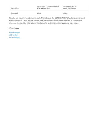
![ALLSELECTED
11/30/2021 • 4 minutes to read
Syntax
ALLSELECTED([<tableName> | <columnName>[, <columnName>[, <columnName>[,…]]]] )
Parameters
TERM DEFINITION
tableName The name of an existing table, using standard DAX syntax.
This parameter cannot be an expression. This parameter is
optional.
columnName The name of an existing column using standard DAX syntax,
usually fully qualified. It cannot be an expression. This
parameter is optional.
Return value
Remarks
Example
Removes context filters from columns and rows in the current query, while retaining all other context filters or
explicit filters.
The ALLSELECTED function gets the context that represents all rows and columns in the query, while keeping
explicit filters and contexts other than row and column filters. This function can be used to obtain visual totals in
queries.
The context of the query without any column and row filters.
If there is one argument, the argument is either tableName or columnName. If there is more than one
argument, they must be columns from the same table.
This function is different from ALL() because it retains all filters explicitly set within the query, and it
retains all context filters other than row and column filters.
This function is not supported for use in DirectQuery mode when used in calculated columns or row-
level security (RLS) rules.
The following example shows how to generate different levels of visual totals in a table report using DAX
expressions. In the report two (2) previous filters have been applied to the Reseller Sales data; one on Sales
Territory Group = Europe and the other on Promotion Type = Volume Discount. Once filters have been applied,
visual totals can be calculated for the entire report, for All Years, or for All Product Categories. Also, for
illustration purposes the grand total for All Reseller Sales is obtained too, removing all filters in the report.
Evaluating the following DAX expression results in a table with all the information needed to build a table with
Visual Totals.](https://image.slidesharecdn.com/funcoesdax-220812141017-bb6cd4dc/85/Funcoes-DAX-pdf-146-320.jpg)
![define
measure 'Reseller Sales'[Reseller Sales Amount]=sum('Reseller Sales'[Sales Amount])
measure 'Reseller Sales'[Reseller Grand Total]=calculate(sum('Reseller Sales'[Sales Amount]), ALL('Reseller
Sales'))
measure 'Reseller Sales'[Reseller Visual Total]=calculate(sum('Reseller Sales'[Sales Amount]),
ALLSELECTED())
measure 'Reseller Sales'[Reseller Visual Total for All of Calendar Year]=calculate(sum('Reseller
Sales'[Sales Amount]), ALLSELECTED('Date'[Calendar Year]))
measure 'Reseller Sales'[Reseller Visual Total for All of Product Category Name]=calculate(sum('Reseller
Sales'[Sales Amount]), ALLSELECTED('Product Category'[Product Category Name]))
evaluate
CalculateTable(
//CT table expression
summarize(
//summarize table expression
crossjoin(distinct('Product Category'[Product Category Name]), distinct('Date'[Calendar Year]))
//First Group by expression
, 'Product Category'[Product Category Name]
//Second Group by expression
, 'Date'[Calendar Year]
//Summary expressions
, "Reseller Sales Amount", [Reseller Sales Amount]
, "Reseller Grand Total", [Reseller Grand Total]
, "Reseller Visual Total", [Reseller Visual Total]
, "Reseller Visual Total for All of Calendar Year", [Reseller Visual Total for All of Calendar Year]
, "Reseller Visual Total for All of Product Category Name", [Reseller Visual Total for All of Product
Category Name]
)
//CT filters
, 'Sales Territory'[Sales Territory Group]="Europe", 'Promotion'[Promotion Type]="Volume Discount"
)
order by [Product Category Name], [Calendar Year]
[PRODUCT
CATEGORY
NAME]
[CALENDAR
YEAR]
[RESELLER
SALES
AMOUNT]
[RESELLER
GRAND
TOTAL]
[RESELLER
VISUAL
TOTAL]
[RESELLER
VISUAL TOTAL
FOR ALL OF
CALENDAR
YEAR]
[RESELLER
VISUAL TOTAL
FOR ALL OF
PRODUCT
CATEGORY
NAME]
Accessories 2000 80450596.98
23
877006.7987 38786.018
Accessories 2001 80450596.98
23
877006.7987 38786.018
Accessories 2002 625.7933 80450596.98
23
877006.7987 38786.018 91495.3104
Accessories 2003 26037.3132 80450596.98
23
877006.7987 38786.018 572927.0136
Accessories 2004 12122.9115 80450596.98
23
877006.7987 38786.018 212584.4747
Accessories 2005 80450596.98
23
877006.7987 38786.018
After executing the above expression in SQL Server Management Studio against AdventureWorks DW Tabular
Model, you obtain the following results:](https://image.slidesharecdn.com/funcoesdax-220812141017-bb6cd4dc/85/Funcoes-DAX-pdf-147-320.jpg)
![Accessories 2006 80450596.98
23
877006.7987 38786.018
Bikes 2000 80450596.98
23
877006.7987 689287.7939
Bikes 2001 80450596.98
23
877006.7987 689287.7939
Bikes 2002 73778.938 80450596.98
23
877006.7987 689287.7939 91495.3104
Bikes 2003 439771.4136 80450596.98
23
877006.7987 689287.7939 572927.0136
Bikes 2004 175737.4423 80450596.98
23
877006.7987 689287.7939 212584.4747
Bikes 2005 80450596.98
23
877006.7987 689287.7939
Bikes 2006 80450596.98
23
877006.7987 689287.7939
Clothing 2000 80450596.98
23
877006.7987 95090.7757
Clothing 2001 80450596.98
23
877006.7987 95090.7757
Clothing 2002 12132.4334 80450596.98
23
877006.7987 95090.7757 91495.3104
Clothing 2003 58234.2214 80450596.98
23
877006.7987 95090.7757 572927.0136
Clothing 2004 24724.1209 80450596.98
23
877006.7987 95090.7757 212584.4747
Clothing 2005 80450596.98
23
877006.7987 95090.7757
Clothing 2006 80450596.98
23
877006.7987 95090.7757
Components 2000 80450596.98
23
877006.7987 53842.2111
Components 2001 80450596.98
23
877006.7987 53842.2111
[PRODUCT
CATEGORY
NAME]
[CALENDAR
YEAR]
[RESELLER
SALES
AMOUNT]
[RESELLER
GRAND
TOTAL]
[RESELLER
VISUAL
TOTAL]
[RESELLER
VISUAL TOTAL
FOR ALL OF
CALENDAR
YEAR]
[RESELLER
VISUAL TOTAL
FOR ALL OF
PRODUCT
CATEGORY
NAME]](https://image.slidesharecdn.com/funcoesdax-220812141017-bb6cd4dc/85/Funcoes-DAX-pdf-148-320.jpg)
![Components 2002 4958.1457 80450596.98
23
877006.7987 53842.2111 91495.3104
Components 2003 48884.0654 80450596.98
23
877006.7987 53842.2111 572927.0136
Components 2004 80450596.98
23
877006.7987 53842.2111 212584.4747
Components 2005 80450596.98
23
877006.7987 53842.2111
Components 2006 80450596.98
23
877006.7987 53842.2111
[PRODUCT
CATEGORY
NAME]
[CALENDAR
YEAR]
[RESELLER
SALES
AMOUNT]
[RESELLER
GRAND
TOTAL]
[RESELLER
VISUAL
TOTAL]
[RESELLER
VISUAL TOTAL
FOR ALL OF
CALENDAR
YEAR]
[RESELLER
VISUAL TOTAL
FOR ALL OF
PRODUCT
CATEGORY
NAME]
NOTE
The columns in the report are:
Reseller Sales Amount
The actual value of Reseller Sales for the year and product category. This value appears in a cell in the center of
your report, at the intersection of year and catergory.
Reseller Visual Total for All of Calendar Year
The total value for a product category across all years. This value appears at the end of a column or row for a
given product category and across all years in the report.
Reseller Visual Total for All of Product Category Name
The total value for a year across all product categories. This value appears at the end of a column or row for a
given year and across all product categories in the report.
Reseller Visual Total
The total value for all years and product categories. This value usually appears in the bottom rightmost corner of
the table.
Reseller Grand Total
This is the grand total for all reseller sales, before any filter has been applied; you should notice the difference
with [Reseller Visual Total]. You do remember that this report includes two (2) filters, one on Product Category
Group and the other in Promotion Type.
if you have explicit filters in your expression, those filters are also applied to the expression.](https://image.slidesharecdn.com/funcoesdax-220812141017-bb6cd4dc/85/Funcoes-DAX-pdf-149-320.jpg)
![CALCULATE
11/30/2021 • 4 minutes to read
NOTE
Syntax
CALCULATE(<expression>[, <filter1> [, <filter2> [, …]]])
Parameters
TERM DEFINITION
expression The expression to be evaluated.
filter1, filter2,… (Optional) Boolean expressions or table expressions that
defines filters, or filter modifier functions.
Boolean filter expressions
Evaluates an expression in a modified filter context.
There's also the CALCULATETABLE function. It performs exactly the same functionality, except it modifies the filter context
applied to an expression that returns a table object.
The expression used as the first parameter is essentially the same as a measure.
Filters can be:
Boolean filter expressions
Table filter expressions
Filter modification functions
When there are multiple filters, they can be evaluated by using the AND (&&) logical operator, meaning all
conditions must be TRUE, or by the OR (||) logical operator, meaning either condition can be true.
A Boolean expression filter is an expression that evaluates to TRUE or FALSE. There are several rules that they
must abide by:
They can reference columns from a single table.
They cannot reference measures.
They cannot use a nested CALCULATE function.
Beginning with the September 2021 release of Power BI Desktop, the following also apply:
They cannot use functions that scan or return a table unless they are passed as arguments to aggregation
functions.
They can contain an aggregation function that returns a scalar value. For example,](https://image.slidesharecdn.com/funcoesdax-220812141017-bb6cd4dc/85/Funcoes-DAX-pdf-150-320.jpg)
![Table filter expression
Filter modifier functions
FUNCTION PURPOSE
REMOVEFILTERS Remove all filters, or filters from one or more columns of a
table, or from all columns of a single table.
ALL , ALLEXCEPT, ALLNOBLANKROW Remove filters from one or more columns, or from all
columns of a single table.
KEEPFILTERS Add filter without removing existing filters on the same
columns.
USERELATIONSHIP Engage an inactive relationship between related columns, in
which case the active relationship will automatically become
inactive.
CROSSFILTER Modify filter direction (from both to single, or from single to
both) or disable a relationship.
Return value
Remarks
Total sales on the last selected date =
CALCULATE (
SUM ( Sales[Sales Amount] ),
'Sales'[OrderDateKey] = MAX ( 'Sales'[OrderDateKey] )
)
A table expression filter applies a table object as a filter. It could be a reference to a model table, but more likely
it's a function that returns a table object. You can use the FILTER function to apply complex filter conditions,
including those that cannot be defined by a Boolean filter expression.
Filter modifier functions allow you to do more than simply add filters. They provide you with additional control
when modifying filter context.
1
The ALL function and its variants behave as both filter modifiers and as functions that return table objects. If
the REMOVEFILTERS function is supported by your tool, it's better to use it to remove filters.
1
The value that is the result of the expression.
When filter expressions are provided, the CALCULATE function modifies the filter context to evaluate the
expression. For each filter expression, there are two possible standard outcomes when the filter
expression is not wrapped in the KEEPFILTERS function:
If the columns (or tables) aren't in the filter context, then new filters will be added to the filter context
to evaluate the expression.
If the columns (or tables) are already in the filter context, the existing filters will be overwritten by the
new filters to evaluate the CALCULATE expression.
The CALCULATE function used without filters achieves a specific requirement. It transitions row context to
filter context. It's required when an expression (not a model measure) that summarizes model data needs
to be evaluated in row context. This scenario can happen in a calculated column formula or when an
expression in an iterator function is evaluated. Note that when a model measure is used in row context,
context transition is automatic.](https://image.slidesharecdn.com/funcoesdax-220812141017-bb6cd4dc/85/Funcoes-DAX-pdf-151-320.jpg)
![Examples
Blue Revenue =
CALCULATE(
SUM(Sales[Sales Amount]),
'Product'[Color] = "Blue"
)
CATEGORY SALES AMOUNT BLUE REVENUE
Accessories $1,272,057.89 $165,406.62
Bikes $94,620,526.21 $8,374,313.88
Clothing $2,117,613.45 $259,488.37
Components $11,799,076.66 $803,642.10
Total $109,809,274.20 $9,602,850.97
CHANNEL SALES AMOUNT REVENUE % TOTAL CHANNEL
Internet $29,358,677.22 26.74%
Reseller $80,450,596.98 73.26%
Total $109,809,274.20 100.00%
Revenue % Total Channel =
DIVIDE(
SUM(Sales[Sales Amount]),
CALCULATE(
SUM(Sales[Sales Amount]),
REMOVEFILTERS('Sales Order'[Channel])
)
)
This function is not supported for use in DirectQuery mode when used in calculated columns or row-
level security (RLS) rules.
The following Sales table measure definition produces a revenue result, but only for products that have the
color blue.
Examples in this article can be added to the Power BI Desktop sample model. To get the model, see DAX sample
model.
The CALCULATE function evaluates the sum of the Sales table Sales Amount column in a modified filter
context. A new filter is added to the Product table Color column—or, the filter overwrites any filter that's
already applied to the column.
The following Sales table measure definition produces a ratio of sales over sales for all sales channels.
The DIVIDE function divides an expression that sums of the Sales table Sales Amount column value (in the
filter context) by the same expression in a modified filter context. It's the CALCULATE function that modifies the
filter context by using the REMOVEFILTERS function, which is a filter modifier function. It removes filters from](https://image.slidesharecdn.com/funcoesdax-220812141017-bb6cd4dc/85/Funcoes-DAX-pdf-152-320.jpg)
![Customer Segment =
IF(
CALCULATE(SUM(Sales[Sales Amount]), ALLEXCEPT(Customer, Customer[CustomerKey])) < 2500,
"Low",
"High"
)
See also
the Sales Order table Channel column.
The following Customer table calculated column definition classifies customers into a loyalty class. It's a very
simple scenario: When the revenue produced by the customer is less than $2500, they're classified as Low;
otherwise they're High.
In this example, row context is converted to the filter context. It's known as context transition. The ALLEXCEPT
function removes filters from all Customer table columns except the CustomerKey column.
Filter context
Row context
CALCULATETABLE function
Filter functions](https://image.slidesharecdn.com/funcoesdax-220812141017-bb6cd4dc/85/Funcoes-DAX-pdf-153-320.jpg)
![CALCULATETABLE
11/30/2021 • 3 minutes to read
NOTE
Syntax
CALCULATETABLE(<expression>[, <filter1> [, <filter2> [, …]]])
Parameters
TERM DEFINITION
expression The table expression to be evaluated.
filter1, filter2,… (Optional) Boolean expressions or table expressions that
defines filters, or filter modifier functions.
Boolean filter expressions
Table filter expression
Evaluates a table expression in a modified filter context.
There's also the CALCULATE function. It performs exactly the same functionality, except it modifies the filter context
applied to an expression that returns a scalar value.
The expression used as the first parameter must be a model table or a function that returns a table.
Filters can be:
Boolean filter expressions
Table filter expressions
Filter modification functions
When there are multiple filters, they're evaluated by using the AND logical operator. That means all conditions
must be TRUE at the same time.
A Boolean expression filter is an expression that evaluates to TRUE or FALSE. There are several rules that they
must abide by:
They can reference only a single column.
They cannot reference measures.
They cannot use a nested CALCULATE function.
Beginning with the September 2021 release of Power BI Desktop, the following also apply:
They cannot use functions that scan or return a table unless they are passed as arguments to aggregation
functions.
They can contain an aggregation function that returns a scalar value.
A table expression filter applies a table object as a filter. It could be a reference to a model table, but more likely
it's a function that returns a table object. You can use the FILTER function to apply complex filter conditions,](https://image.slidesharecdn.com/funcoesdax-220812141017-bb6cd4dc/85/Funcoes-DAX-pdf-154-320.jpg)
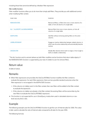
![= SUMX(
CALCULATETABLE(
'InternetSales_USD',
'DateTime'[CalendarYear] = 2006
),
[SalesAmount_USD]
)
ROW LABELS
INTERNET
SALESAMOUNT_USD
CALCULATETABLE 2006
INTERNET SALES
INTERNET SALES TO 2006
RATIO
2005 $2,627,031.40 $5,681,440.58 0.46
2006 $5,681,440.58 $5,681,440.58 1.00
2007 $8,705,066.67 $5,681,440.58 1.53
2008 $9,041,288.80 $5,681,440.58 1.59
Grand Total $26,054,827.45 $5,681,440.58 4.59
See also
It results in the following table:
Filter context
CALCULATE function (DAX)
Filter functions (DAX)](https://image.slidesharecdn.com/funcoesdax-220812141017-bb6cd4dc/85/Funcoes-DAX-pdf-156-320.jpg)
![21 Jerseys $699,429.78 7
33 Lights 36
34 Locks $15,059.47 33
1 Mountain Bikes $34,305,864.29 2
12 Mountain Frames $4,511,170.68 4
35 Panniers 36
13 Pedals $140,422.20 19
36 Pumps $12,695.18 34
2 Road Bikes $40,551,696.34 1
14 Road Frames $3,636,398.71 5
15 Saddles $52,526.47 26
22 Shorts $385,707.80 10
23 Socks $28,337.85 31
24 Tights $189,179.37 16
37 Tires and Tubes $224,832.81 13
3 Touring Bikes $13,334,864.18 3
16 Touring Frames $1,545,344.02 6
25 Vests $240,990.04 11
17 Wheels $648,240.04 8
PRODUCTSUBCATEGORYKE
Y
ENGLISHPRODUCTSUBCATE
GORYNAME TOTALSUBCATEGORYSALES SUBCATEGORYRANKING
Creating a Rank Value
= COUNTROWS(FILTER(ProductSubcategory, EARLIER(ProductSubcategory[TotalSubcategorySales])
<ProductSubcategory[TotalSubcategorySales]))+1
One way to obtain a rank value for a given value in a row is to count the number of rows, in the same table, that
have a value larger (or smaller) than the one that is being compared. This technique returns a blank or zero
value for the highest value in the table, whereas equal values will have the same rank value and next value (after
the equal values) will have a non consecutive rank value. See the sample below.
A new calculated column, SubCategorySalesRanking, is created by using the following formula.](https://image.slidesharecdn.com/funcoesdax-220812141017-bb6cd4dc/85/Funcoes-DAX-pdf-159-320.jpg)
![See also
The following steps describe the method of calculation in more detail.
1. The EARLIER function gets the value of TotalSubcategorySales for the current row in the table. In this
case, because the process is starting, it is the first row in the table
2. EARLIER([TotalSubcategorySales]) evaluates to $156,167.88, the current row in the outer loop.
3. The FILTER function now returns a table where all rows have a value of TotalSubcategorySales larger
than $156,167.88 (which is the current value for EARLIER).
4. The COUNTROWS function counts the rows of the filtered table and assigns that value to the new
calculated column in the current row plus 1. Adding 1 is needed to prevent the top ranked value from
become a Blank.
5. The calculated column formula moves to the next row and repeats steps 1 to 4. These steps are repeated
until the end of the table is reached.
The EARLIER function will always get the value of the column prior to the current table operation. If you need to
get a value from the loop before that, set the second argument to 2.
EARLIEST function
Filter functions](https://image.slidesharecdn.com/funcoesdax-220812141017-bb6cd4dc/85/Funcoes-DAX-pdf-160-320.jpg)
![FILTER
11/30/2021 • 2 minutes to read
Syntax
FILTER(<table>,<filter>)
Parameters
TERM DEFINITION
table The table to be filtered. The table can also be an expression
that results in a table.
filter A Boolean expression that is to be evaluated for each row of
the table. For example, [Amount] > 0 or
[Region] = "France"
Return value
Remarks
Example
FILTER('InternetSales_USD', RELATED('SalesTerritory'[SalesTerritoryCountry])<>"United States")
Returns a table that represents a subset of another table or expression.
A table containing only the filtered rows.
You can use FILTER to reduce the number of rows in the table that you are working with, and use only
specific data in calculations. FILTER is not used independently, but as a function that is embedded in other
functions that require a table as an argument.
For best practices when using FILTER, see Avoid using FILTER as a filter argument.
Use COUNTROWS instead of COUNT in DAX
This function is not supported for use in DirectQuery mode when used in calculated columns or row-level
security (RLS) rules.
The following example creates a report of Internet sales outside the United States by using a measure that filters
out sales in the United States, and then slicing by calendar year and product categories. To create this measure,
you filter the table, Internet Sales USD, by using Sales Territory, and then use the filtered table in a SUMX
function.
In this example, the expression:
Returns a table that is a subset of Internet Sales minus all rows that belong to the United States sales territory.
The RELATED function is what links the Territory key in the Internet Sales table to SalesTerritoryCountry in the](https://image.slidesharecdn.com/funcoesdax-220812141017-bb6cd4dc/85/Funcoes-DAX-pdf-162-320.jpg)
![Table 1. Comparing total sales for U.S. vs. all other regions
ROW LABELS INTERNET SALES NON USA INTERNET SALES
Australia $4,999,021.84 $4,999,021.84
Canada $1,343,109.10 $1,343,109.10
France $2,490,944.57 $2,490,944.57
Germany $2,775,195.60 $2,775,195.60
United Kingdom $5,057,076.55 $5,057,076.55
United States $9,389,479.79
Grand Total $26,054,827.45 $16,665,347.67
Table 2. Comparing non- U.S. sales by product categories
ROW LABELS ACCESSORIES BIKES CLOTHING GRAND TOTAL
2005 $1,526,481.95 $1,526,481.95
2006 $3,554,744.04 $3,554,744.04
2007 $156,480.18 $5,640,106.05 $70,142.77 $5,866,729.00
2008 $228,159.45 $5,386,558.19 $102,675.04 $5,717,392.68
Grand Total $384,639.63 $16,107,890.23 $172,817.81 $16,665,347.67
SUMX(FILTER('InternetSales_USD', RELATED('SalesTerritory'[SalesTerritoryCountry])<>"United States")
,'InternetSales_USD'[SalesAmount_USD])
See also
SalesTerritory table.
The following table demonstrates the proof of concept for the measure, NON USA Internet Sales, the formula
for which is provided in the code section below. The table compares all Internet sales with non- USA Internet
sales, to show that the filter expression works, by excluding United States sales from the computation.
To re-create this table, add the field, SalesTerritoryCountry, to the Row Labels area of a report or PivotTable.
The final report table shows the results when you create a PivotTable by using the measure, NON USA Internet
Sales. Add the field, CalendarYear, to the Row Labels area of the PivotTable and add the field,
ProductCategoryName, to the Column Labels area.
Filter functions
ALL function
ALLEXCEPT function](https://image.slidesharecdn.com/funcoesdax-220812141017-bb6cd4dc/85/Funcoes-DAX-pdf-163-320.jpg)
![EVALUATE ROW(
"$$ in WA"
, CALCULATE('Internet Sales'[Internet Total Sales]
, 'Geography'[State Province Code]="WA"
)
, "$$ in WA and OR"
, CALCULATE('Internet Sales'[Internet Total Sales]
, 'Geography'[State Province Code]="WA"
|| 'Geography'[State Province Code]="OR"
)
, "$$ in WA and BC"
, CALCULATE('Internet Sales'[Internet Total Sales]
, 'Geography'[State Province Code]="WA"
|| 'Geography'[State Province Code]="BC"
)
, "$$ in WA and OR ??"
, CALCULATE(
CALCULATE('Internet Sales'[Internet Total Sales]
,'Geography'[State Province Code]="WA"
|| 'Geography'[State Province Code]="OR"
)
, 'Geography'[State Province Code]="WA"
|| 'Geography'[State Province Code]="BC"
)
, "$$ in WA !!"
, CALCULATE(
CALCULATE('Internet Sales'[Internet Total Sales]
, KEEPFILTERS('Geography'[State Province Code]="WA"
|| 'Geography'[State Province Code]="OR"
)
)
, 'Geography'[State Province Code]="WA"
|| 'Geography'[State Province Code]="BC"
)
)
COLUMN VALUE
[$$ in WA] $ 2,467,248.34
[$$ in WA and OR] $ 3,638,239.88
[$$ in WA and BC] $ 4,422,588.44
[$$ in WA and OR ??] $ 3,638,239.88
[$$ in WA !!] $ 2,467,248.34
Internet Sales for the state of Washington and the province of British Columbia (both regions combined).
The fourth expression calculates Internet Sales for Washington and Oregon, while the filter for Washington and
British Columbia is applied.
The next expression calculates Internet Sales for Washington and Oregon but uses KEEPFILTERS; the filter for
Washington and British Columbia is part of the prior context.
When this expression is evaluated against the sample database AdventureWorks DW, the following results are
obtained.](https://image.slidesharecdn.com/funcoesdax-220812141017-bb6cd4dc/85/Funcoes-DAX-pdf-165-320.jpg)
![NOTE
See also
The above results were formatted to a table, instead of a single row, for educational purposes.
First, examine the expression, [$$ in WA and OR ??]. You might wonder how this formula could return the
value for sales in Washington and Oregon, since the outer CALCULATE expression includes a filter for
Washington and British Columbia. The answer is that the default behavior of CALCULATE overrides the outer
filters in 'Geography'[State Province Code] and substitutes its own filter arguments, because the filters apply to
the same column.
Next, examine the expression, [$$ in WA !!]. You might wonder how this formula could return the value for
sales in Washington and nothing else, since the argument filter includes Oregon and the outer CALCULATE
expression includes a filter in Washington and British Columbia. The answer is that KEEPFILTERS modifies the
default behavior of CALCULATE and adds an additional filter. Because the intersection of filters is used, now the
outer filter 'Geography'[State Province Code]="WA" || 'Geography'[State Province Code]="BC") is
added to the filter argument 'Geography'[State Province Code]="WA" || 'Geography'[State Province
Code]="OR",. Because both filters apply to the same column, the resulting filter 'Geography'[State Province
Code]="WA" is the filter that is applied when evaluating the expression.
Filter functions
CALCULATE function
CALCULATETABLE function](https://image.slidesharecdn.com/funcoesdax-220812141017-bb6cd4dc/85/Funcoes-DAX-pdf-166-320.jpg)
![LOOKUPVALUE
11/30/2021 • 2 minutes to read
Syntax
LOOKUPVALUE(
<result_columnName>,
<search_columnName>,
<search_value>
[, <search2_columnName>, <search2_value>]…
[, <alternateResult>]
)
Parameters
TERM DEFINITION
result_columnName The name of an existing column that contains the value you
want to return. It cannot be an expression.
search_columnName The name of an existing column. It can be in the same table
as result_columnName or in a related table. It cannot be an
expression.
search_value The value to search for in search_columnName.
alternateResult (Optional) The value returned when the context for
result_columnName has been filtered down to zero or more
than one distinct value. When not provided, the function
returns BLANK when result_columnName is filtered down to
zero value or an error when more than one distinct value.
Return value
Remarks
Returns the value for the row that meets all criteria specified by one or more search conditions.
The value of result_column at the row where all pairs of search_column and search_value have an exact
match.
If there's no match that satisfies all the search values, BLANK or alternateResult (if supplied) is returned. In
other words, the function won't return a lookup value if only some of the criteria match.
If multiple rows match the search values and in all cases result_column values are identical, then that value is
returned. However, if result_column returns different values, an error or alternateResult (if supplied) is
returned.
If there is a relationship between the result and search tables, in most cases, using RELATED function
instead of LOOKUPVALUE is more efficient and provides better performance.
The search_value and alternateResult parameters are evaluated before the function iterates through](https://image.slidesharecdn.com/funcoesdax-220812141017-bb6cd4dc/85/Funcoes-DAX-pdf-167-320.jpg)
![Example
CHANNEL = LOOKUPVALUE('Sales Order'[Channel],'Sales Order'[SalesOrderLineKey],[SalesOrderLineKey])
CHANNEL = RELATED('Sales Order'[Channel])
See also
the rows of the search table.
Avoid using ISERROR or IFERROR functions to capture an error returned by LOOKUPVALUE. If some
inputs to the function will result in an error when a single output value cannot be determined, providing
an alternateResult parameter is the most reliable and highest performing way to handle the error.
This function is not supported for use in DirectQuery mode when used in calculated columns or row-
level security (RLS) rules.
Examples in this article can be added to the Power BI Desktop sample model. To get the model, see DAX sample
model.
The following calculated column defined in the Sales table uses the LOOKUPVALUE function to return channel
values from the Sales Order table.
However, in this case, because there is a relationship between the Sales Order and Sales tables, it's more
efficient to use the RELATED function.
RELATED function (DAX)
Information functions](https://image.slidesharecdn.com/funcoesdax-220812141017-bb6cd4dc/85/Funcoes-DAX-pdf-168-320.jpg)
![REMOVEFILTERS
11/30/2021 • 2 minutes to read
Syntax
REMOVEFILTERS([<table> | <column>[, <column>[, <column>[,…]]]])
Parameters
TERM DEFINITION
table The table that you want to clear filters on.
column The column that you want to clear filters on.
Return value
Remarks
Example 1
DEFINE
MEASURE FactInternetSales[TotalSales] = SUM(FactInternetSales[SalesAmount])
MEASURE FactInternetSales[%Sales] = DIVIDE([TotalSales], CALCULATE([TotalSales],REMOVEFILTERS()))
EVALUATE
SUMMARIZECOLUMNS(
ROLLUPADDISSUBTOTAL(DimProductCategory[EnglishProductCategoryName], "IsGrandTotal"),
"TotalSales", [TotalSales],
"%Sales", [%Sales]
)
ORDER BY
[IsGrandTotal] DESC, [TotalSales] DESC
Clear filters from the specified tables or columns.
N/A. See remarks.
REMOVEFILTERS can only be used to clear filters but not to return a table.
This function is not supported for use in DirectQuery mode when used in calculated columns or row-
level security (RLS) rules.
DAX query
Returns](https://image.slidesharecdn.com/funcoesdax-220812141017-bb6cd4dc/85/Funcoes-DAX-pdf-169-320.jpg)
![DIMPRODUCTCATEGORY[E
NGLISHPRODUCTCATEGOR
YNAME] [ISGRANDTOTAL] [TOTALSALES] [%SALES]
Row1 True 29358677.2207 1
Bikes False 28318144.6507 0.964557920570538
Accessories False 700759.96 0.023868921434441
Clothing False 339772.61 0.0115731579950215
Example 2
DEFINE
MEASURE FactInternetSales[TotalSales] = SUM(FactInternetSales[SalesAmount])
MEASURE FactInternetSales[%Sales] = DIVIDE([TotalSales],
CALCULATE([TotalSales],REMOVEFILTERS(DimProductSubcategory[EnglishProductSubcategoryName])))
EVALUATE
SUMMARIZECOLUMNS(
DimProductCategory[EnglishProductCategoryName],
DimProductSubcategory[EnglishProductSubcategoryName],
"TotalSales", [TotalSales],
"%Sales", [%Sales]
)
ORDER BY
DimProductCategory[EnglishProductCategoryName] ASC,
DimProductSubcategory[EnglishProductSubcategoryName] ASC
DIMPRODUCTCATEGORY
[ENGLISHPRODUCTCATEGO
RYNAME]
DIMPRODUCTSUBCATEGOR
Y
[ENGLISHPRODUCTSUBCAT
EGORYNAME] [TOTALSALES] [%SALES]
Accessories Bike Racks 39360 0.05616759
Accessories Bike Stands 39591 0.05649723
Accessories Bottles and Cages 56798.19 0.08105228
Accessories Cleaners 7218.6 0.0103011
Accessories Fenders 46619.58 0.06652717
Accessories Helmets 225335.6 0.3215589
Accessories Hydration Packs 40307.67 0.05751994
Accessories Tires and Tubes 245529.32 0.35037578
Bikes Mountain Bikes 9952759.564 0.35146228
DAX query
Returns](https://image.slidesharecdn.com/funcoesdax-220812141017-bb6cd4dc/85/Funcoes-DAX-pdf-170-320.jpg)
![Bikes Road Bikes 14520584.04 0.51276608
Bikes Touring Bikes 3844801.05 0.13577164
Clothing Caps 19688.1 0.05794493
Clothing Gloves 35020.7 0.10307099
Clothing Jerseys 172950.68 0.5090189
Clothing Shorts 71319.81 0.20990453
Clothing Socks 5106.32 0.01502864
Clothing Vests 35687 0.10503201
DIMPRODUCTCATEGORY
[ENGLISHPRODUCTCATEGO
RYNAME]
DIMPRODUCTSUBCATEGOR
Y
[ENGLISHPRODUCTSUBCAT
EGORYNAME] [TOTALSALES] [%SALES]](https://image.slidesharecdn.com/funcoesdax-220812141017-bb6cd4dc/85/Funcoes-DAX-pdf-171-320.jpg)
![SELECTEDVALUE
11/30/2021 • 2 minutes to read
Syntax
SELECTEDVALUE(<columnName>[, <alternateResult>])
Parameters
TERM DEFINITION
columnName The name of an existing column, using standard DAX syntax.
It cannot be an expression.
alternateResult (Optional) The value returned when the context for
columnName has been filtered down to zero or more than
one distinct value. When not provided, the default value is
BLANK().
Return value
Remarks
Example
DEFINE
MEASURE DimProduct[Selected Color] = SELECTEDVALUE(DimProduct[Color], "No Single Selection")
EVALUATE
SUMMARIZECOLUMNS
(ROLLUPADDISSUBTOTAL(DimProduct[Color], "Is Total"),
"Selected Color", [Selected Color])ORDER BY [Is Total] ASC,
[Color] ASC
Returns the value when the context for columnName has been filtered down to one distinct value only.
Otherwise returns alternateResult.
The value when the context for columnName has been filtered down to one distinct value only. Else,
alternateResult.
An equivalent expression for SELECTEDVALUE(<columnName>, <alternateResult>) is
IF(HASONEVALUE(<columnName>), VALUES(<columnName>), <alternateResult>) .
To learn more about best practices when using SELECTEDVALUE, see Use SELECTEDVALUE instead of
VALUES in DAX.
This function is not supported for use in DirectQuery mode when used in calculated columns or row-
level security (RLS) rules.
The following DAX query:
Returns the following:](https://image.slidesharecdn.com/funcoesdax-220812141017-bb6cd4dc/85/Funcoes-DAX-pdf-172-320.jpg)
![DIMPRODUCT[COLOR] [IS TOTAL] [SELECTED COLOR]
Black FALSE Black
Blue FALSE Blue
Grey FALSE Grey
Multi FALSE Multi
NA FALSE NA
Red FALSE Red
Silver FALSE Silver
Silver/Black FALSE Silver/Black
White FALSE White
Yellow FALSE Yellow
TRUE No Single Selection](https://image.slidesharecdn.com/funcoesdax-220812141017-bb6cd4dc/85/Funcoes-DAX-pdf-173-320.jpg)
![ACCRINT
11/30/2021 • 2 minutes to read
Syntax
ACCRINT(<issue>, <first_interest>, <settlement>, <rate>, <par>, <frequency>[, <basis>[, <calc_method>]])
Parameters
TERM DEFINITION
issue The security's issue date.
first_interest The security's first interest date.
settlement The security's settlement date. The security settlement date
is the date after the issue date when the security is traded to
the buyer.
rate The security's annual coupon rate.
par The security's par value.
frequency The number of coupon payments per year. For annual
payments, frequency = 1; for semiannual, frequency = 2; for
quarterly, frequency = 4.
basis (Optional) The type of day count basis to use. If basis is
omitted, it is assumed to be 0. The accepted values are listed
below this table.
calc_method (Optional) A logical value that specifies the way to calculate
the total accrued interest when the date of settlement is
later than the date of first_interest. If calc_method is omitted,
it is assumed to be TRUE.
- If calc_method evaluates to TRUE or is omitted, ACCRINT
returns the total accrued interest from issue to settlement.
- If calc_method evaluates to FALSE, ACCRINT returns the
accrued interest from first_interest to settlement.
BASIS DAY COUNT BASIS
0 or omitted US (NASD) 30/360
1 Actual/actual
2 Actual/360
Returns the accrued interest for a security that pays periodic interest.
The basis parameter accepts the following values:](https://image.slidesharecdn.com/funcoesdax-220812141017-bb6cd4dc/85/Funcoes-DAX-pdf-178-320.jpg)
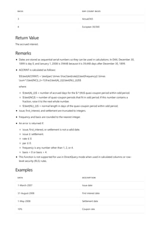
![1000 Par value
2 Frequency is semiannual (see above)
0 30/360 basis (see above)
DATA DESCRIPTION
Example 1
EVALUATE
{
ACCRINT(DATE(2007,3,1), DATE(2008,8,31), DATE(2008,5,1), 0.1, 1000, 2, 0)
}
[VALUE]
116.944444444444
Example 2
EVALUATE
{
ACCRINT(DATE(2007,3,1), DATE(2008,8,31), DATE(2008,5,1), 0.1, 1000, 2, 0, FALSE)
}
[VALUE]
66.9444444444445
The following DAX query:
Returns the accrued interest from issue to settlement, for a security with the terms specified above.
The following DAX query:
Returns the accrued interest from first_interest to settlement, for a security with the terms specified above.](https://image.slidesharecdn.com/funcoesdax-220812141017-bb6cd4dc/85/Funcoes-DAX-pdf-180-320.jpg)
![ACCRINTM
11/30/2021 • 2 minutes to read
Syntax
ACCRINTM(<issue>, <maturity>, <rate>, <par>[, <basis>])
Parameters
TERM DEFINITION
issue The security's issue date.
maturity The security's maturity date.
rate The security's annual coupon rate.
par The security's par value.
basis (Optional) The type of day count basis to use. If basis is
omitted, it is assumed to be 0. The accepted values are listed
below this table.
BASIS DAY COUNT BASIS
0 or omitted US (NASD) 30/360
1 Actual/actual
2 Actual/360
3 Actual/365
4 European 30/360
Return Value
Remarks
Returns the accrued interest for a security that pays interest at maturity.
The basis parameter accepts the following values:
The accrued interest.
Dates are stored as sequential serial numbers so they can be used in calculations. In DAX, December 30,
1899 is day 0, and January 1, 2008 is 39448 because it is 39,448 days after December 30, 1899.
ACCRINTM is calculated as follows:](https://image.slidesharecdn.com/funcoesdax-220812141017-bb6cd4dc/85/Funcoes-DAX-pdf-181-320.jpg)
![Example
DATA DESCRIPTION
1-April-2008 Issue date
15-June-2008 Maturity date
10% Percent coupon
1000 Par value
3 Actual/365 basis (see above)
EVALUATE
{
ACCRINTM(DATE(2008,4,1), DATE(2008,6,15), 0.1, 1000, 3)
}
[VALUE]
20.5479452054795
$$text{ACCRINTM} = text{par} times text{rate} times frac{text{A}}{text{D}}$$
where:
$text{A}$ = Number of accrued days counted according to a monthly basis. For interest at maturity
items, the number of days from the issue date to the maturity date is used.
$text{D}$ = Annual Year Basis.
issue and maturity are truncated to integers.
basis is rounded to the nearest integer.
An error is returned if:
issue or maturity is not a valid date.
issue ≥ maturity.
rate ≤ 0.
par ≤ 0.
basis < 0 or basis > 4.
This function is not supported for use in DirectQuery mode when used in calculated columns or row-
level security (RLS) rules.
The following DAX query:
Returns the accrued interest for a security with the terms specified above.](https://image.slidesharecdn.com/funcoesdax-220812141017-bb6cd4dc/85/Funcoes-DAX-pdf-182-320.jpg)
![AMORDEGRC
11/30/2021 • 2 minutes to read
Syntax
AMORDEGRC(<cost>, <date_purchased>, <first_period>, <salvage>, <period>, <rate>[, <basis>])
Parameters
TERM DEFINITION
cost The cost of the asset.
date_purchased The date of the purchase of the asset.
first_period The date of the end of the first period.
salvage The salvage value at the end of the life of the asset.
period The period.
rate The rate of depreciation.
basis (Optional) The type of day count basis to use. If basis is
omitted, it is assumed to be 0. The accepted values are listed
below this table.
BASIS DATE SYSTEM
0 or omitted 360 days (NASD method)
1 Actual
3 365 days in a year
4 360 days in a year (European method)
Return Value
Returns the depreciation for each accounting period. This function is provided for the French accounting system.
If an asset is purchased in the middle of the accounting period, the prorated depreciation is taken into account.
The function is similar to AMORLINC, except that a depreciation coefficient is applied in the calculation
depending on the life of the assets.
The basis parameter accepts the following values:
The depreciation for each accounting period.](https://image.slidesharecdn.com/funcoesdax-220812141017-bb6cd4dc/85/Funcoes-DAX-pdf-183-320.jpg)
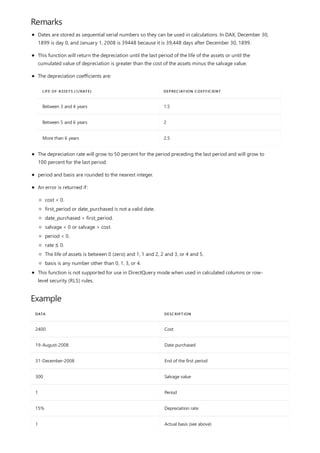
![EVALUATE
{
AMORDEGRC(2400, DATE(2008,8,19), DATE(2008,12,31), 300, 1, 0.15, 1)
}
[VALUE]
776
The following DAX query:
Returns the first period's depreciation, given the terms specified above.](https://image.slidesharecdn.com/funcoesdax-220812141017-bb6cd4dc/85/Funcoes-DAX-pdf-185-320.jpg)
![AMORLINC
11/30/2021 • 2 minutes to read
Syntax
AMORLINC(<cost>, <date_purchased>, <first_period>, <salvage>, <period>, <rate>[, <basis>])
Parameters
TERM DEFINITION
cost The cost of the asset.
date_purchased The date of the purchase of the asset.
first_period The date of the end of the first period.
salvage The salvage value at the end of the life of the asset.
period The period.
rate The rate of depreciation.
basis (Optional) The type of day count basis to use. If basis is
omitted, it is assumed to be 0. The accepted values are listed
below this table.
BASIS DATE SYSTEM
0 or omitted 360 days (NASD method)
1 Actual
3 365 days in a year
4 360 days in a year (European method)
Return Value
Remarks
Returns the depreciation for each accounting period. This function is provided for the French accounting system.
If an asset is purchased in the middle of the accounting period, the prorated depreciation is taken into account.
The basis parameter accepts the following values:
The depreciation for each accounting period.
Dates are stored as sequential serial numbers so they can be used in calculations. In DAX, December 30,](https://image.slidesharecdn.com/funcoesdax-220812141017-bb6cd4dc/85/Funcoes-DAX-pdf-186-320.jpg)
![Example
DATA DESCRIPTION
2400 Cost
19-August-2008 Date purchased
31-December-2008 End of the first period
300 Salvage value
1 Period
15% Depreciation rate
1 Actual basis (see above)
EVALUATE
{
AMORLINC(2400, DATE(2008,8,19), DATE(2008,12,31), 300, 1, 0.15, 1)
}
[VALUE]
360
1899 is day 0, and January 1, 2008 is 39448 because it is 39,448 days after December 30, 1899.
period and basis are rounded to the nearest integer.
An error is returned if:
cost < 0.
first_period or date_purchased is not a valid date.
date_purchased > first_period.
salvage < 0 or salvage > cost.
period < 0.
rate ≤ 0.
basis is any number other than 0, 1, 3, or 4.
This function is not supported for use in DirectQuery mode when used in calculated columns or row-
level security (RLS) rules.
The following DAX query:
Returns the first period's depreciation, given the terms specified above.](https://image.slidesharecdn.com/funcoesdax-220812141017-bb6cd4dc/85/Funcoes-DAX-pdf-187-320.jpg)
![COUPDAYBS
11/30/2021 • 2 minutes to read
Syntax
COUPDAYBS(<settlement>, <maturity>, <frequency>[, <basis>])
Parameters
TERM DEFINITION
settlement The security's settlement date. The security settlement date
is the date after the issue date when the security is traded to
the buyer.
maturity The security's maturity date. The maturity date is the date
when the security expires.
frequency The number of coupon payments per year. For annual
payments, frequency = 1; for semiannual, frequency = 2; for
quarterly, frequency = 4.
basis (Optional) The type of day count basis to use. If basis is
omitted, it is assumed to be 0. The accepted values are listed
below this table.
BASIS DAY COUNT BASIS
0 or omitted US (NASD) 30/360
1 Actual/actual
2 Actual/360
3 Actual/365
4 European 30/360
Return Value
Remarks
Returns the number of days from the beginning of a coupon period until its settlement date.
The basis parameter accepts the following values:
The number of days from the beginning of a coupon period until its settlement date.
Dates are stored as sequential serial numbers so they can be used in calculations. In DAX, December 30,
1899 is day 0, and January 1, 2008 is 39448 because it is 39,448 days after December 30, 1899.](https://image.slidesharecdn.com/funcoesdax-220812141017-bb6cd4dc/85/Funcoes-DAX-pdf-188-320.jpg)
![Example
DATA DESCRIPTION
25-Jan-11 Settlement date
15-Nov-11 Maturity date
2 Semiannual coupon (see above)
1 Actual/actual basis (see above)
EVALUATE
{
COUPDAYBS(DATE(2011,1,25), DATE(2011,11,15), 2, 1)
}
[VALUE]
71
The settlement date is the date a buyer purchases a coupon, such as a bond. The maturity date is the date
when a coupon expires. For example, suppose a 30-year bond is issued on January 1, 2008, and is
purchased by a buyer six months later. The issue date would be January 1, 2008, the settlement date
would be July 1, 2008, and the maturity date would be January 1, 2038, 30 years after the January 1,
2008, issue date.
settlement and maturity are truncated to integers.
frequency and basis are rounded to the nearest integer.
An error is returned if:
settlement or maturity is not a valid date.
settlement ≥ maturity.
frequency is any number other than 1, 2, or 4.
basis < 0 or basis > 4.
This function is not supported for use in DirectQuery mode when used in calculated columns or row-
level security (RLS) rules.
The following DAX query:
Returns the number of days from the beginning of the coupon period until the settlement date, for a bond with
terms above.](https://image.slidesharecdn.com/funcoesdax-220812141017-bb6cd4dc/85/Funcoes-DAX-pdf-189-320.jpg)
![COUPDAYS
11/30/2021 • 2 minutes to read
Syntax
COUPDAYS(<settlement>, <maturity>, <frequency>[, <basis>])
Parameters
TERM DEFINITION
settlement The security's settlement date. The security settlement date
is the date after the issue date when the security is traded to
the buyer.
maturity The security's maturity date. The maturity date is the date
when the security expires.
frequency The number of coupon payments per year. For annual
payments, frequency = 1; for semiannual, frequency = 2; for
quarterly, frequency = 4.
basis (Optional) The type of day count basis to use. If basis is
omitted, it is assumed to be 0. The accepted values are listed
below this table.
BASIS DAY COUNT BASIS
0 or omitted US (NASD) 30/360
1 Actual/actual
2 Actual/360
3 Actual/365
4 European 30/360
Return Value
Remarks
Returns the number of days in the coupon period that contains the settlement date.
The basis parameter accepts the following values:
The number of days in the coupon period that contains the settlement date.
Dates are stored as sequential serial numbers so they can be used in calculations. In DAX, December 30,
1899 is day 0, and January 1, 2008 is 39448 because it is 39,448 days after December 30, 1899.](https://image.slidesharecdn.com/funcoesdax-220812141017-bb6cd4dc/85/Funcoes-DAX-pdf-190-320.jpg)
![Example
DATA DESCRIPTION
25-Jan-11 Settlement date
15-Nov-11 Maturity date
2 Semiannual coupon (see above)
1 Actual/actual basis (see above)
EVALUATE
{
COUPDAYS(DATE(2011,1,25), DATE(2011,11,15), 2, 1)
}
[VALUE]
181
The settlement date is the date a buyer purchases a coupon, such as a bond. The maturity date is the date
when a coupon expires. For example, suppose a 30-year bond is issued on January 1, 2008, and is
purchased by a buyer six months later. The issue date would be January 1, 2008, the settlement date
would be July 1, 2008, and the maturity date is January 1, 2038, 30 years after the January 1, 2008 issue
date.
settlement and maturity are truncated to integers.
frequency and basis are rounded to the nearest integer.
An error is returned if:
settlement or maturity is not a valid date.
settlement ≥ maturity.
frequency is any number other than 1, 2, or 4.
basis < 0 or basis > 4.
This function is not supported for use in DirectQuery mode when used in calculated columns or row-
level security (RLS) rules.
The following DAX query:
Returns the number of days in the coupon period that contains the settlement date, for a bond with the terms
specified above.](https://image.slidesharecdn.com/funcoesdax-220812141017-bb6cd4dc/85/Funcoes-DAX-pdf-191-320.jpg)
![COUPDAYSNC
11/30/2021 • 2 minutes to read
Syntax
COUPDAYSNC(<settlement>, <maturity>, <frequency>[, <basis>])
Parameters
TERM DEFINITION
settlement The security's settlement date. The security settlement date
is the date after the issue date when the security is traded to
the buyer.
maturity The security's maturity date. The maturity date is the date
when the security expires.
frequency The number of coupon payments per year. For annual
payments, frequency = 1; for semiannual, frequency = 2; for
quarterly, frequency = 4.
basis (Optional) The type of day count basis to use. If basis is
omitted, it is assumed to be 0. The accepted values are listed
below this table.
BASIS DAY COUNT BASIS
0 or omitted US (NASD) 30/360
1 Actual/actual
2 Actual/360
3 Actual/365
4 European 30/360
Return Value
Remarks
Returns the number of days from the settlement date to the next coupon date.
The basis parameter accepts the following values:
The number of days from the settlement date to the next coupon date.
Dates are stored as sequential serial numbers so they can be used in calculations. In DAX, December 30,
1899 is day 0, and January 1, 2008 is 39448 because it is 39,448 days after December 30, 1899.](https://image.slidesharecdn.com/funcoesdax-220812141017-bb6cd4dc/85/Funcoes-DAX-pdf-192-320.jpg)
![Example
DATA DESCRIPTION
25-Jan-11 Settlement date
15-Nov-11 Maturity date
2 Semiannual coupon (see above)
1 Actual/actual basis (see above)
EVALUATE
{
COUPDAYSNC(DATE(2011,1,25), DATE(2011,11,15), 2, 1)
}
[VALUE]
110
The settlement date is the date a buyer purchases a coupon, such as a bond. The maturity date is the date
when a coupon expires. For example, suppose a 30-year bond is issued on January 1, 2008, and is
purchased by a buyer six months later. The issue date would be January 1, 2008, the settlement date
would be July 1, 2008, and the maturity date would be January 1, 2038, which is 30 years after the
January 1, 2008, issue date.
settlement and maturity are truncated to integers.
frequency and basis are rounded to the nearest integer.
An error is returned if:
settlement or maturity is not a valid date.
settlement ≥ maturity.
frequency is any number other than 1, 2, or 4.
basis < 0 or basis > 4.
This function is not supported for use in DirectQuery mode when used in calculated columns or row-
level security (RLS) rules.
The following DAX query:
Returns the number of days from the settlement date to the next coupon date, for a bond with the terms
specified above.](https://image.slidesharecdn.com/funcoesdax-220812141017-bb6cd4dc/85/Funcoes-DAX-pdf-193-320.jpg)
![COUPNCD
11/30/2021 • 2 minutes to read
Syntax
COUPNCD(<settlement>, <maturity>, <frequency>[, <basis>])
Parameters
TERM DEFINITION
settlement The security's settlement date. The security settlement date
is the date after the issue date when the security is traded to
the buyer.
maturity The security's maturity date. The maturity date is the date
when the security expires.
frequency The number of coupon payments per year. For annual
payments, frequency = 1; for semiannual, frequency = 2; for
quarterly, frequency = 4.
basis (Optional) The type of day count basis to use. If basis is
omitted, it is assumed to be 0. The accepted values are listed
below this table.
BASIS DAY COUNT BASIS
0 or omitted US (NASD) 30/360
1 Actual/actual
2 Actual/360
3 Actual/365
4 European 30/360
Return Value
Remarks
Returns the next coupon date after the settlement date.
The basis parameter accepts the following values:
The next coupon date after the settlement date.
Dates are stored as sequential serial numbers so they can be used in calculations. In DAX, December 30,
1899 is day 0, and January 1, 2008 is 39448 because it is 39,448 days after December 30, 1899.](https://image.slidesharecdn.com/funcoesdax-220812141017-bb6cd4dc/85/Funcoes-DAX-pdf-194-320.jpg)
![Example
DATA DESCRIPTION
25-Jan-11 Settlement date
15-Nov-11 Maturity date
2 Semiannual coupon (see above)
1 Actual/actual basis (see above)
EVALUATE
{
COUPNCD(DATE(2011,1,25), DATE(2011,11,15), 2, 1)
}
[VALUE]
5/15/2011 12:00:00 AM
The settlement date is the date a buyer purchases a coupon, such as a bond. The maturity date is the date
when a coupon expires. For example, suppose a 30-year bond is issued on January 1, 2008, and is
purchased by a buyer six months later. The issue date would be January 1, 2008, the settlement date
would be July 1, 2008, and the maturity date is January 1, 2038, 30 years after the January 1, 2008 issue
date.
settlement and maturity are truncated to integers.
frequency and basis are rounded to the nearest integer.
An error is returned if:
settlement or maturity is not a valid date.
settlement ≥ maturity.
frequency is any number other than 1, 2, or 4.
basis < 0 or basis > 4.
This function is not supported for use in DirectQuery mode when used in calculated columns or row-
level security (RLS) rules.
The following DAX query:
Returns the next coupon date after the settlement date, for a bond with the terms specified above.](https://image.slidesharecdn.com/funcoesdax-220812141017-bb6cd4dc/85/Funcoes-DAX-pdf-195-320.jpg)
![COUPNUM
11/30/2021 • 2 minutes to read
Syntax
COUPNUM(<settlement>, <maturity>, <frequency>[, <basis>])
Parameters
TERM DEFINITION
settlement The security's settlement date. The security settlement date
is the date after the issue date when the security is traded to
the buyer.
maturity The security's maturity date. The maturity date is the date
when the security expires.
frequency The number of coupon payments per year. For annual
payments, frequency = 1; for semiannual, frequency = 2; for
quarterly, frequency = 4.
basis (Optional) The type of day count basis to use. If basis is
omitted, it is assumed to be 0. The accepted values are listed
below this table.
BASIS DAY COUNT BASIS
0 or omitted US (NASD) 30/360
1 Actual/actual
2 Actual/360
3 Actual/365
4 European 30/360
Return Value
Remarks
Returns the number of coupons payable between the settlement date and maturity date, rounded up to the
nearest whole coupon.
The basis parameter accepts the following values:
The number of coupons payable between the settlement date and maturity date.
Dates are stored as sequential serial numbers so they can be used in calculations. In DAX, December 30,](https://image.slidesharecdn.com/funcoesdax-220812141017-bb6cd4dc/85/Funcoes-DAX-pdf-196-320.jpg)
![Example
DATA DESCRIPTION
25-Jan-07 Settlement date
15-Nov-08 Maturity date
2 Semiannual coupon (see above)
1 Actual/actual basis (see above)
EVALUATE
{
COUPNUM(DATE(2007,1,25), DATE(2008,11,15), 2, 1)
}
[VALUE]
4
1899 is day 0, and January 1, 2008 is 39448 because it is 39,448 days after December 30, 1899.
The settlement date is the date a buyer purchases a coupon, such as a bond. The maturity date is the date
when a coupon expires. For example, suppose a 30-year bond is issued on January 1, 2008, and is
purchased by a buyer six months later. The issue date would be January 1, 2008, the settlement date
would be July 1, 2008, and the maturity date would be January 1, 2038, which is 30 years after the
January 1, 2008, issue date.
settlement and maturity are truncated to integers.
frequency and basis are rounded to the nearest integer.
An error is returned if:
settlement or maturity is not a valid date.
settlement ≥ maturity.
frequency is any number other than 1, 2, or 4.
basis < 0 or basis > 4.
This function is not supported for use in DirectQuery mode when used in calculated columns or row-
level security (RLS) rules.
The following DAX query:
Returns the number of coupon payments for a bond with the terms specified above.](https://image.slidesharecdn.com/funcoesdax-220812141017-bb6cd4dc/85/Funcoes-DAX-pdf-197-320.jpg)
![COUPPCD
11/30/2021 • 2 minutes to read
Syntax
COUPPCD(<settlement>, <maturity>, <frequency>[, <basis>])
Parameters
TERM DEFINITION
settlement The security's settlement date. The security settlement date
is the date after the issue date when the security is traded to
the buyer.
maturity The security's maturity date. The maturity date is the date
when the security expires.
frequency The number of coupon payments per year. For annual
payments, frequency = 1; for semiannual, frequency = 2; for
quarterly, frequency = 4.
basis (Optional) The type of day count basis to use. If basis is
omitted, it is assumed to be 0. The accepted values are listed
below this table.
BASIS DAY COUNT BASIS
0 or omitted US (NASD) 30/360
1 Actual/actual
2 Actual/360
3 Actual/365
4 European 30/360
Return Value
Remarks
Returns the previous coupon date before the settlement date.
The basis parameter accepts the following values:
The previous coupon date before the settlement date.
Dates are stored as sequential serial numbers so they can be used in calculations. In DAX, December 30,
1899 is day 0, and January 1, 2008 is 39448 because it is 39,448 days after December 30, 1899.](https://image.slidesharecdn.com/funcoesdax-220812141017-bb6cd4dc/85/Funcoes-DAX-pdf-198-320.jpg)
![Example
DATA DESCRIPTION
25-Jan-11 Settlement date
15-Nov-11 Maturity date
2 Semiannual coupon (see above)
1 Actual/actual basis (see above)
EVALUATE
{
COUPPCD(DATE(2011,1,25), DATE(2011,11,15), 2, 1)
}
[VALUE]
11/15/2010 12:00:00 AM
The settlement date is the date a buyer purchases a coupon, such as a bond. The maturity date is the date
when a coupon expires. For example, suppose a 30-year bond is issued on January 1, 2008, and is
purchased by a buyer six months later. The issue date would be January 1, 2008, the settlement date
would be July 1, 2008, and the maturity date would be January 1, 2038, which is 30 years after the
January 1, 2008, issue date.
settlement and maturity are truncated to integers.
frequency and basis are rounded to the nearest integer.
An error is returned if:
settlement or maturity is not a valid date.
settlement ≥ maturity.
frequency is any number other than 1, 2, or 4.
basis < 0 or basis > 4.
This function is not supported for use in DirectQuery mode when used in calculated columns or row-
level security (RLS) rules.
The following DAX query:
Returns the previous coupon date before the settlement date, for a bond using the terms specified above.](https://image.slidesharecdn.com/funcoesdax-220812141017-bb6cd4dc/85/Funcoes-DAX-pdf-199-320.jpg)

![Examples
DATA DESCRIPTION
9% Annual interest rate
30 Years of the loan
125000 Present value
Example 1
EVALUATE
{
CUMIPMT(0.09/12, 30*12, 125000, 13, 24, 1)
}
[VALUE]
-11052.3395838718
Example 2
EVALUATE
{
CUMIPMT(0.09/12, 30*12, 125000, 1, 1, 0)
}
[VALUE]
-937.5
rate ≤ 0.
nper < 1.
pv ≤ 0.
start_period < 1 or start_period > end_period.
end_period < start_period or end_period > nper.
type is any number other than 0 or 1.
This function is not supported for use in DirectQuery mode when used in calculated columns or row-
level security (RLS) rules.
The following DAX query:
Returns the total interest paid in the second year of payments, periods 13 through 24, assuming that the
payments are made at the beginning of each month.
The following DAX query:
Returns the interest paid in a single payment in the first month, assuming that the payment is made at the end
of the month.](https://image.slidesharecdn.com/funcoesdax-220812141017-bb6cd4dc/85/Funcoes-DAX-pdf-201-320.jpg)
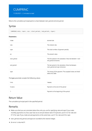
![Examples
DATA DESCRIPTION
9% Annual interest rate
30 Term in years
125000 Present value
Example 1
EVALUATE
{
CUMPRINC(0.09/12, 30*12, 125000, 13, 24, 1)
}
[VALUE]
-927.153472378062
Example 2
EVALUATE
{
CUMPRINC(0.09/12, 30*12, 125000, 1, 1, 0)
}
[VALUE]
-68.2782711809784
rate ≤ 0.
nper < 1.
pv ≤ 0.
start_period < 1 or start_period > end_period.
end_period < start_period or end_period > nper.
type is any number other than 0 or 1.
This function is not supported for use in DirectQuery mode when used in calculated columns or row-
level security (RLS) rules.
The following DAX query:
Returns the total principal paid in the second year of payments, periods 13 through 24, assuming the payments
are made at the beginning of each month.
The following DAX query:
Returns the principal paid in a single payment in the first month, assuming the payment is made at the end of
the month.](https://image.slidesharecdn.com/funcoesdax-220812141017-bb6cd4dc/85/Funcoes-DAX-pdf-203-320.jpg)
![DB
11/30/2021 • 2 minutes to read
Syntax
DB(<cost>, <salvage>, <life>, <period>[, <month>])
Parameters
TERM DEFINITION
cost The initial cost of the asset.
salvage The value at the end of the depreciation (sometimes called
the salvage value of the asset). This value can be 0.
life The number of periods over which the asset is being
depreciated (sometimes called the useful life of the asset).
period The period for which you want to calculate the depreciation.
Period must use the same units as life. Must be between 1
and life (inclusive).
month (Optional) The number of months in the first year. If month
is omitted, it is assumed to be 12.
Return Value
Remarks
Returns the depreciation of an asset for a specified period using the fixed-declining balance method.
The depreciation over the specified period.
The fixed-declining balance method computes depreciation at a fixed rate. DB uses the following formulas
to calculate depreciation for a period:
$$(text{cost} - text{total depreciation from prior periods}) times text{rate}$$
where:
$text{rate} = 1 - ((frac{text{salvage}}{text{cost}})^{(frac{1}{text{life}})})text{, rounded to three
decimal places}$
Depreciation for the first and last periods is a special case.
For the first period, DB uses this formula:
$$frac{text{cost} times text{rate} times text{month}}{12}$$
For the last period, DB uses this formula:
$$frac{(text{cost} - text{total depreciation from prior periods}) times text{rate} times (12 -](https://image.slidesharecdn.com/funcoesdax-220812141017-bb6cd4dc/85/Funcoes-DAX-pdf-204-320.jpg)
![Examples
Example 1
EVALUATE
{
DB(1000000, 0, 6, 1, 2)
}
[VALUE]
166666.666666667
Example 2
DEFINE
VAR NumDepreciationPeriods = MAX(Asset[LifeTimeYears])+1
VAR DepreciationPeriods = GENERATESERIES(1, NumDepreciationPeriods)
EVALUATE
ADDCOLUMNS (
DepreciationPeriods,
"Current Period Total Depreciation",
SUMX (
FILTER (
Asset,
[Value] <= [LifetimeYears]+1
),
DB([InitialCost], [SalvageValue], [LifetimeYears], [Value], 7)
)
)
text{month})}{12}$$
period and month are rounded to the nearest integer.
An error is returned if:
cost < 0.
salvage < 0.
life < 1.
period < 1 or period > life.
month < 1 or month > 12.
This function is not supported for use in DirectQuery mode when used in calculated columns or row-
level security (RLS) rules.
The following DAX query:
Returns an asset's depreciation in the last two months of the first year, assuming it will be worth $0 after 6
years.
The following calculates the total depreciation of all assets in different years over their lifetimes. Here, the first
year only includes 7 months of depreciation, and the last year only includes 5 months.](https://image.slidesharecdn.com/funcoesdax-220812141017-bb6cd4dc/85/Funcoes-DAX-pdf-205-320.jpg)
![DDB
11/30/2021 • 2 minutes to read
Syntax
DDB(<cost>, <salvage>, <life>, <period>[, <factor>])
Parameters
TERM DEFINITION
cost The initial cost of the asset.
salvage The value at the end of the depreciation (sometimes called
the salvage value of the asset). This value can be 0.
life The number of periods over which the asset is being
depreciated (sometimes called the useful life of the asset).
period The period for which you want to calculate the depreciation.
Period must use the same units as life. Must be between 1
and life (inclusive).
factor (Optional) The rate at which the balance declines. If factor is
omitted, it is assumed to be 2 (the double-declining balance
method).
Return Value
Remarks
Returns the depreciation of an asset for a specified period using the double-declining balance method or some
other method you specify.
The depreciation over the specified period.
The double-declining balance method computes depreciation at an accelerated rate. Depreciation is
highest in the first period and decreases in successive periods. DDB uses the following formula to
calculate depreciation for a period:
$$text{Min}((text{cost} - text{total depreciation from prior periods}) times (frac{text{factor}}
{text{life}}),(text{cost} - text{salvage} - text{total depreciation from prior periods}))$$
Change factor if you do not want to use the double-declining balance method.
Use the VDB function if you want to switch to the straight-line depreciation method when depreciation is
greater than the declining balance calculation.
period is rounded to the nearest integer.
An error is returned if:](https://image.slidesharecdn.com/funcoesdax-220812141017-bb6cd4dc/85/Funcoes-DAX-pdf-206-320.jpg)
![Examples
Example 1
EVALUATE
{
DDB(1000000, 0, 10, 5, 1.5)
}
[VALUE]
78300.9375
Example 2
DEFINE
VAR NumDepreciationPeriods = MAX(Asset[LifeTimeYears])
VAR DepreciationPeriods = GENERATESERIES(1, NumDepreciationPeriods)
EVALUATE
ADDCOLUMNS (
DepreciationPeriods,
"Current Period Total Depreciation",
SUMX (
FILTER (
Asset,
[Value] <= [LifetimeYears]
),
DDB([InitialCost], [SalvageValue], [LifetimeYears], [Value])
)
)
cost < 0.
salvage < 0.
life < 1.
period < 1 or period > life.
factor ≤ 0.
This function is not supported for use in DirectQuery mode when used in calculated columns or row-
level security (RLS) rules.
The following DAX query:
Returns an asset's depreciation in the 5$^{th}$ year, assuming it will be worth $0 after 10 years. This
calculation uses a factor of 1.5.
The following calculates the total depreciation of all assets in different years over their lifetimes. This calculation
uses the default factor of 2 (the double-declining balance method).](https://image.slidesharecdn.com/funcoesdax-220812141017-bb6cd4dc/85/Funcoes-DAX-pdf-207-320.jpg)
![DISC
11/30/2021 • 2 minutes to read
Syntax
DISC(<settlement>, <maturity>, <pr>, <redemption>[, <basis>])
Parameters
TERM DEFINITION
settlement The security's settlement date. The security settlement date
is the date after the issue date when the security is traded to
the buyer.
maturity The security's maturity date. The maturity date is the date
when the security expires.
pr The security's price per $100 face value.
redemption The security's redemption value per $100 face value.
basis (Optional) The type of day count basis to use. If basis is
omitted, it is assumed to be 0. The accepted values are listed
below this table.
BASIS DAY COUNT BASIS
0 or omitted US (NASD) 30/360
1 Actual/actual
2 Actual/360
3 Actual/365
4 European 30/360
Return Value
Remarks
Returns the discount rate for a security.
The basis parameter accepts the following values:
The discount rate.
Dates are stored as sequential serial numbers so they can be used in calculations. In DAX, December 30,
1899 is day 0, and January 1, 2008 is 39448 because it is 39,448 days after December 30, 1899.](https://image.slidesharecdn.com/funcoesdax-220812141017-bb6cd4dc/85/Funcoes-DAX-pdf-208-320.jpg)

![[VALUE]
0.000686384169121348](https://image.slidesharecdn.com/funcoesdax-220812141017-bb6cd4dc/85/Funcoes-DAX-pdf-210-320.jpg)
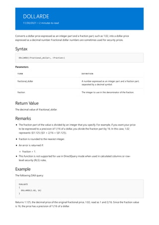
![DURATION
11/30/2021 • 2 minutes to read
Syntax
DURATION(<settlement>, <maturity>, <coupon>, <yld>, <frequency>[, <basis>])
Parameters
TERM DEFINITION
settlement The security's settlement date. The security settlement date
is the date after the issue date when the security is traded to
the buyer.
maturity The security's maturity date. The maturity date is the date
when the security expires.
coupon The security's annual coupon rate.
yld The security's annual yield.
frequency The number of coupon payments per year. For annual
payments, frequency = 1; for semiannual, frequency = 2; for
quarterly, frequency = 4.
basis (Optional) The type of day count basis to use. If basis is
omitted, it is assumed to be 0. The accepted values are listed
below this table.
BASIS DAY COUNT BASIS
0 or omitted US (NASD) 30/360
1 Actual/actual
2 Actual/360
3 Actual/365
4 European 30/360
Return Value
Returns the Macauley duration for an assumed par value of $100. Duration is defined as the weighted average
of the present value of cash flows, and is used as a measure of a bond price's response to changes in yield.
The basis parameter accepts the following values:
The Macauley duration.](https://image.slidesharecdn.com/funcoesdax-220812141017-bb6cd4dc/85/Funcoes-DAX-pdf-213-320.jpg)
![Remarks
Example
DATA DESCRIPTION
07/01/2018 Settlement date
01/01/2048 Maturity date
8.0% Percent coupon
9.0% Percent yield
2 Frequency is semiannual (see above)
1 Actual/actual basis (see above)
EVALUATE
{
DURATION(DATE(2018,7,1), DATE(2048,1,1), 0.08, 0.09, 2, 1)
}
[VALUE]
10.9191452815919
Dates are stored as sequential serial numbers so they can be used in calculations. In DAX, December 30,
1899 is day 0, and January 1, 2008 is 39448 because it is 39,448 days after December 30, 1899.
The settlement date is the date a buyer purchases a coupon, such as a bond. The maturity date is the date
when a coupon expires. For example, suppose a 30-year bond is issued on January 1, 2008, and is
purchased by a buyer six months later. The issue date would be January 1, 2008, the settlement date
would be July 1, 2008, and the maturity date is January 1, 2038, which is 30 years after the January 1,
2008, issue date.
settlement and maturity are truncated to integers.
frequency, and basis are rounded to the nearest integer.
An error is returned if:
settlement or maturity is not a valid date.
settlement ≥ maturity.
coupon < 0.
yld < 0
frequency is any number other than 1, 2, or 4.
basis < 0 or basis > 4.
This function is not supported for use in DirectQuery mode when used in calculated columns or row-
level security (RLS) rules.
The following DAX query:
Returns the Macauley duration for a bond with the terms specified above.](https://image.slidesharecdn.com/funcoesdax-220812141017-bb6cd4dc/85/Funcoes-DAX-pdf-214-320.jpg)
![EVALUATE
{
EFFECT(0.0525, 4)
}
[VALUE]
0.0535426673707584
Returns the effective interest rate using the terms specified above.](https://image.slidesharecdn.com/funcoesdax-220812141017-bb6cd4dc/85/Funcoes-DAX-pdf-216-320.jpg)
![FV
11/30/2021 • 2 minutes to read
Syntax
FV(<rate>, <nper>, <pmt>[, <pv>[, <type>]])
Parameters
TERM DEFINITION
rate The interest rate per period.
nper The total number of payment periods in an annuity.
pmt The payment made each period; it cannot change over the
life of the annuity. Typically, pmt contains principal and
interest but no other fees or taxes.
pv (Optional) The present value, or the lump-sum amount that
a series of future payments is worth right now. If pv is
omitted, it is assumed to be BLANK.
type (Optional) The number 0 or 1 which indicates when
payments are due. If type is omitted, it is assumed to be 0.
The accepted values are listed below this table.
SET TYPE EQUAL TO IF PAYMENTS ARE DUE
0 or omitted At the end of the period
1 At the beginning of the period
Return Value
Remarks
Calculates the future value of an investment based on a constant interest rate. You can use FV with either
periodic, constant payments, and/or a single lump sum payment.
The type parameter accepts the following values:
Note: For a more complete description of the arguments in FV and for more information on annuity functions,
see the PV function.
The future value of an investment.
Make sure that you are consistent about the units you use for specifying rate and nper. If you make
monthly payments on a four-year loan at 12 percent annual interest, use 0.12/12 for rate and 4*12 for
nper. If you make annual payments on the same loan, use 0.12 for rate and 4 for nper.](https://image.slidesharecdn.com/funcoesdax-220812141017-bb6cd4dc/85/Funcoes-DAX-pdf-217-320.jpg)
![Example
DATA DESCRIPTION
6% Annual interest rate
10 Number of payments
-200 Amount of the payment
-500 Present value
1 Payment is due at the beginning of the period (0 indicates
payment is due at end of period)
EVALUATE
{
FV(0.06/12, 10, -200, -500, 1)
}
[VALUE]
2581.40337406012
For all the arguments, cash you pay out, such as deposits to savings, is represented by negative numbers;
cash you receive, such as dividend checks, is represented by positive numbers.
type is rounded to the nearest integer.
An error is returned if:
nper < 1
This function is not supported for use in DirectQuery mode when used in calculated columns or row-
level security (RLS) rules.
The following DAX query:
Returns the future value of an investment using the terms specified above.](https://image.slidesharecdn.com/funcoesdax-220812141017-bb6cd4dc/85/Funcoes-DAX-pdf-218-320.jpg)
![INTRATE
11/30/2021 • 2 minutes to read
Syntax
INTRATE(<settlement>, <maturity>, <investment>, <redemption>[, <basis>])
Parameters
TERM DEFINITION
settlement The security's settlement date. The security settlement date
is the date after the issue date when the security is traded to
the buyer.
maturity The security's maturity date. The maturity date is the date
when the security expires.
investment The amount invested in the security.
redemption The amount to be received at maturity.
basis (Optional) The type of day count basis to use. If basis is
omitted, it is assumed to be 0. The accepted values are listed
below this table.
BASIS DAY COUNT BASIS
0 or omitted US (NASD) 30/360
1 Actual/actual
2 Actual/360
3 Actual/365
4 European 30/360
Return Value
Remarks
Returns the interest rate for a fully invested security.
The basis parameter accepts the following values:
The interest rate.
Dates are stored as sequential serial numbers so they can be used in calculations. In DAX, December 30,
1899 is day 0, and January 1, 2008 is 39448 because it is 39,448 days after December 30, 1899.](https://image.slidesharecdn.com/funcoesdax-220812141017-bb6cd4dc/85/Funcoes-DAX-pdf-219-320.jpg)
![[VALUE]
0.05768](https://image.slidesharecdn.com/funcoesdax-220812141017-bb6cd4dc/85/Funcoes-DAX-pdf-221-320.jpg)
![IPMT
11/30/2021 • 2 minutes to read
Syntax
IPMT(<rate>, <per>, <nper>, <pv>[, <fv>[, <type>]])
Parameters
TERM DEFINITION
rate The interest rate per period.
per The period for which you want to find the interest. Must be
between 1 and nper (inclusive).
nper The total number of payment periods in an annuity.
pv The present value, or the lump-sum amount that a series of
future payments is worth right now.
fv (Optional) The future value, or a cash balance you want to
attain after the last payment is made. If fv is omitted, it is
assumed to be BLANK.
type (Optional) The number 0 or 1 which indicates when
payments are due. If type is omitted, it is assumed to be 0.
The accepted values are listed below this table.
SET TYPE EQUAL TO IF PAYMENTS ARE DUE
0 or omitted At the end of the period
1 At the beginning of the period
Return Value
Remarks
Returns the interest payment for a given period for an investment based on periodic, constant payments and a
constant interest rate.
The type parameter accepts the following values:
The interest payment for the given period.
Make sure that you are consistent about the units you use for specifying rate and nper. If you make
monthly payments on a four-year loan at 12 percent annual interest, use 0.12/12 for rate and 4*12 for
nper. If you make annual payments on the same loan, use 0.12 for rate and 4 for nper.](https://image.slidesharecdn.com/funcoesdax-220812141017-bb6cd4dc/85/Funcoes-DAX-pdf-222-320.jpg)
![Examples
DATA DESCRIPTION
10.00% Annual interest
3 Years of loan
$8,000 Present value of loan
Example 1
EVALUATE
{
IPMT(0.1/12, 1, 3*12, 8000)
}
[VALUE]
-66.6666666666667
Example 2
EVALUATE
{
IPMT(0.1, 3, 3, 8000)
}
[VALUE]
-292.447129909366
For all the arguments, cash you pay out, such as deposits to savings, is represented by negative numbers;
cash you receive, such as dividend checks, is represented by positive numbers.
type is rounded to the nearest integer.
An error is returned if:
per < 1 or per > nper
nper < 1
This function is not supported for use in DirectQuery mode when used in calculated columns or row-
level security (RLS) rules.
The following DAX query:
Returns the monthly interest due in the first month for a loan with the terms specified above.
The following DAX query:
Returns the yearly interest due in the last year for a loan with the terms specified above, where payments are
made yearly.](https://image.slidesharecdn.com/funcoesdax-220812141017-bb6cd4dc/85/Funcoes-DAX-pdf-223-320.jpg)
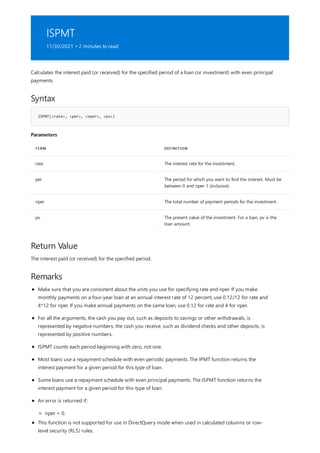
![Example
DATA DESCRIPTION
$4,000 Present value
4 Number of periods
10% Rate
PERIOD PRINCIPAL PAYMENT INTEREST PAYMENT TOTAL PAYMENT BALANCE
4,000.00
1 1,000.00 400.00 1,400.00 3,000.00
2 1,000.00 300.00 1,300.00 2,000.00
3 1,000.00 200.00 1,200.00 1,000.00
4 1,000.00 100.00 1,100.00 0.00
DEFINE
VAR NumPaymentPeriods = 4
VAR PaymentPeriods = GENERATESERIES(0, NumPaymentPeriods-1)
EVALUATE
ADDCOLUMNS (
PaymentPeriods,
"Interest Payment",
ISPMT(0.1, [Value], NumPaymentPeriods, 4000)
)
[VALUE] [INTEREST PAYMENT]
0 -400
1 -300
2 -200
3 -100
To illustrate when to use ISPMT, the amortization table below uses an even-principal repayment schedule with
the terms specified above. The interest charge each period is equal to the rate times the unpaid balance for the
previous period. And the payment each period is equal to the even principal plus the interest for the period.
The following DAX query:
Returns the interest paid during each period, using the even-principal repayment schedule and terms specified
above. The values are negative to indicate that it is interest paid, not received.](https://image.slidesharecdn.com/funcoesdax-220812141017-bb6cd4dc/85/Funcoes-DAX-pdf-225-320.jpg)
![MDURATION
11/30/2021 • 2 minutes to read
Syntax
MDURATION(<settlement>, <maturity>, <coupon>, <yld>, <frequency>[, <basis>])
Parameters
TERM DEFINITION
settlement The security's settlement date. The security settlement date
is the date after the issue date when the security is traded to
the buyer.
maturity The security's maturity date. The maturity date is the date
when the security expires.
coupon The security's annual coupon rate.
yld The security's annual yield.
frequency The number of coupon payments per year. For annual
payments, frequency = 1; for semiannual, frequency = 2; for
quarterly, frequency = 4.
basis (Optional) The type of day count basis to use. If basis is
omitted, it is assumed to be 0. The accepted values are listed
below this table.
BASIS DAY COUNT BASIS
0 or omitted US (NASD) 30/360
1 Actual/actual
2 Actual/360
3 Actual/365
4 European 30/360
Return Value
Returns the modified Macauley duration for a security with an assumed par value of $100.
The basis parameter accepts the following values:
The modified Macauley duration.](https://image.slidesharecdn.com/funcoesdax-220812141017-bb6cd4dc/85/Funcoes-DAX-pdf-226-320.jpg)
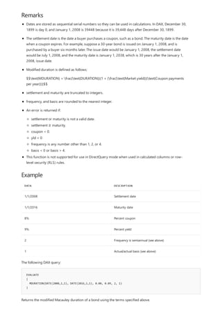
![[VALUE]
5.73566981391884](https://image.slidesharecdn.com/funcoesdax-220812141017-bb6cd4dc/85/Funcoes-DAX-pdf-228-320.jpg)
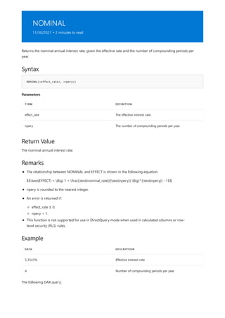
![EVALUATE
{
NOMINAL(0.053543, 4)
}
[VALUE]
0.052500319868356
Returns the nominal interest rate, using the terms specified above.](https://image.slidesharecdn.com/funcoesdax-220812141017-bb6cd4dc/85/Funcoes-DAX-pdf-230-320.jpg)
![NPER
11/30/2021 • 2 minutes to read
Syntax
NPER(<rate>, <pmt>, <pv>[, <fv>[, <type>]])
Parameters
TERM DEFINITION
rate The interest rate per period.
pmt The payment made each period; it cannot change over the
life of the annuity. Typically, pmt contains principal and
interest but no other fees or taxes.
pv The present value, or the lump-sum amount that a series of
future payments is worth right now.
fv (Optional) The future value, or a cash balance you want to
attain after the last payment is made. If fv is omitted, it is
assumed to be BLANK.
type (Optional) The number 0 or 1 and indicates when payments
are due. If type is omitted, it is assumed to be 0. The
accepted values are listed below this table.
SET TYPE EQUAL TO IF PAYMENTS ARE DUE
0 or omitted At the end of the period
1 At the beginning of the period
Return Value
Remarks
Returns the number of periods for an investment based on periodic, constant payments and a constant interest
rate.
The type parameter accepts the following values:
The number of periods for an investment.
type is rounded to the nearest integer.
This function is not supported for use in DirectQuery mode when used in calculated columns or row-
level security (RLS) rules.](https://image.slidesharecdn.com/funcoesdax-220812141017-bb6cd4dc/85/Funcoes-DAX-pdf-231-320.jpg)
![Example
DATA DESCRIPTION
12% Annual interest rate
-100 Payment made each period
-1000 Present value
10000 Future value
1 Payment is due at the beginning of the period (see above)
EVALUATE
{
NPER(0.12/12, -100, -1000, 10000, 1)
}
[VALUE]
59.6738656742946
The following DAX query:
Returns the number of periods for the investment described by the terms specified above.](https://image.slidesharecdn.com/funcoesdax-220812141017-bb6cd4dc/85/Funcoes-DAX-pdf-232-320.jpg)
![ODDFPRICE
11/30/2021 • 4 minutes to read
Syntax
ODDFPRICE(<settlement>, <maturity>, <issue>, <first_coupon>, <rate>, <yld>, <redemption>, <frequency>[,
<basis>])
Parameters
TERM DEFINITION
settlement The security's settlement date. The security settlement date
is the date after the issue date when the security is traded to
the buyer.
maturity The security's maturity date. The maturity date is the date
when the security expires.
issue The security's issue date.
first_coupon The security's first coupon date.
rate The security's interest rate.
yld The security's annual yield.
redemption The security's redemption value per $100 face value.
frequency The number of coupon payments per year. For annual
payments, frequency = 1; for semiannual, frequency = 2; for
quarterly, frequency = 4.
basis (Optional) The type of day count basis to use. If basis is
omitted, it is assumed to be 0. The accepted values are listed
below this table.
BASIS DAY COUNT BASIS
0 or omitted US (NASD) 30/360
1 Actual/actual
2 Actual/360
3 Actual/365
Returns the price per $100 face value of a security having an odd (short or long) first period.
The basis parameter accepts the following values:](https://image.slidesharecdn.com/funcoesdax-220812141017-bb6cd4dc/85/Funcoes-DAX-pdf-233-320.jpg)
![4 European 30/360
BASIS DAY COUNT BASIS
Return Value
Remarks
The price per $100 face value.
Dates are stored as sequential serial numbers so they can be used in calculations. In DAX, December 30,
1899 is day 0, and January 1, 2008 is 39448 because it is 39,448 days after December 30, 1899.
The settlement date is the date a buyer purchases a coupon, such as a bond. The maturity date is the date
when a coupon expires. For example, suppose a 30-year bond is issued on January 1, 2008, and is
purchased by a buyer six months later. The issue date would be January 1, 2008, the settlement date
would be July 1, 2008, and the maturity date would be January 1, 2038, which is 30 years after the
January 1, 2008, issue date.
ODDFPRICE is calculated as follows:
Odd short first coupon:
$$text{ODDFPRICE} = bigg[ frac{text{redemption}}{(1 + frac{text{yld}}{text{frequency}})^{(N - 1 +
frac{text{DSC}}{text{E}})}} bigg] + bigg[ frac{100 times frac{text{rate}}{text{frequency}} times
frac{text{DFC}}{text{E}}}{(1 + frac{text{yld}}{text{frequency}})^{(frac{text{DSC}}{text{E}})}} bigg] +
bigg[ sum^{N}_{k=2} frac{100 times frac{text{rate}}{text{frequency}}}{(1 + frac{text{yld}}
{text{frequency}})^{(k - 1 + frac{text{DSC}}{text{E}})}} bigg] - Big[ 100 times frac{text{rate}}
{text{frequency}} times frac{text{A}}{text{E}} Big] $$
where:
$text{A}$ = number of days from the beginning of the coupon period to the settlement date (accrued
days).
$text{DSC}$ = number of days from the settlement to the next coupon date.
$text{DFC}$ = number of days from the beginning of the odd first coupon to the first coupon date.
$text{E}$ = number of days in the coupon period.
$text{N}$ = number of coupons payable between the settlement date and the redemption date. (If
this number contains a fraction, it is raised to the next whole number.)
Odd long first coupon:
$$text{ODDFPRICE} = bigg[ frac{text{redemption}}{(1 + frac{text{yld}}{text{frequency}})^{(text{N} +
text{N}_{q} + frac{text{DSC}}{text{E}})}} bigg] + bigg[ frac{100 times frac{text{rate}}
{text{frequency}} times Big[ sum^{text{NC}}_{i=1} frac{text{DC}_{i}}{text{NL}_{i}} Big] }{(1 +
frac{text{yld}}{text{frequency}})^{(text{N}_{q} + frac{text{DSC}}{text{E}})}} bigg] + bigg[
sum^{text{N}}_{k=1} frac{100 times frac{text{rate}}{text{frequency}}}{(1 + frac{text{yld}}
{text{frequency}})^{(k - text{N}_{q} + frac{text{DSC}}{text{E}})}} bigg] - Big[ 100 times
frac{text{rate}}{text{frequency}} times sum^{text{NC}}_{i=1} frac{text{A}_{i}}{text{NL}_{i}} Big]$$
where:
$text{A}_{i}$ = number of days from the beginning of the $i^{th}$, or last, quasi-coupon period
within odd period.
$text{DC}_{i}$ = number of days from dated date (or issue date) to first quasi-coupon ($i = 1$) or
number of days in quasi-coupon ($i = 2$,..., $i = text{NC}$).](https://image.slidesharecdn.com/funcoesdax-220812141017-bb6cd4dc/85/Funcoes-DAX-pdf-234-320.jpg)
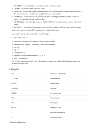
![EVALUATE
{
ODDFPRICE(DATE(2008,11,11), DATE(2021,3,1), DATE(2008,10,15), DATE(2009,3,1), 0.0785, 0.0625, 100.00, 2,
1)
}
[VALUE]
113.597717474079
Returns the price per $100 face value of a security having an odd (short or long) first period, using the terms
specified above.](https://image.slidesharecdn.com/funcoesdax-220812141017-bb6cd4dc/85/Funcoes-DAX-pdf-236-320.jpg)
![ODDFYIELD
11/30/2021 • 2 minutes to read
Syntax
ODDFYIELD(<settlement>, <maturity>, <issue>, <first_coupon>, <rate>, <pr>, <redemption>, <frequency>[,
<basis>])
Parameters
TERM DEFINITION
settlement The security's settlement date. The security settlement date
is the date after the issue date when the security is traded to
the buyer.
maturity The security's maturity date. The maturity date is the date
when the security expires.
issue The security's issue date.
first_coupon The security's first coupon date.
rate The security's interest rate.
pr The security's price.
redemption The security's redemption value per $100 face value.
frequency The number of coupon payments per year. For annual
payments, frequency = 1; for semiannual, frequency = 2; for
quarterly, frequency = 4.
basis (Optional) The type of day count basis to use. If basis is
omitted, it is assumed to be 0. The accepted values are listed
below this table.
BASIS DAY COUNT BASIS
0 or omitted US (NASD) 30/360
1 Actual/actual
2 Actual/360
3 Actual/365
Returns the yield of a security that has an odd (short or long) first period.
The basis parameter accepts the following values:](https://image.slidesharecdn.com/funcoesdax-220812141017-bb6cd4dc/85/Funcoes-DAX-pdf-237-320.jpg)
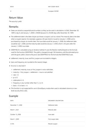
![84.50 Price
100 Redemptive value
2 Frequency is semiannual
0 30/360 basis
DATA ARGUMENT DESCRIPTION
EVALUATE
{
ODDFYIELD(DATE(2008,11,11), DATE(2021,3,1), DATE(2008,10,15), DATE(2009,3,1), 0.0575, 84.50, 100, 2, 0)
}
[VALUE]
0.0772455415972989
The following DAX query:
Returns the yield of a security that has an odd (short or long) first period, using the terms specified above.](https://image.slidesharecdn.com/funcoesdax-220812141017-bb6cd4dc/85/Funcoes-DAX-pdf-239-320.jpg)
![ODDLPRICE
11/30/2021 • 2 minutes to read
Syntax
ODDLPRICE(<settlement>, <maturity>, <last_interest>, <rate>, <yld>, <redemption>, <frequency>[, <basis>])
Parameters
TERM DEFINITION
settlement The security's settlement date. The security settlement date
is the date after the issue date when the security is traded to
the buyer.
maturity The security's maturity date. The maturity date is the date
when the security expires.
last_interest The security's last coupon date.
rate The security's interest rate.
yld The security's annual yield.
redemption The security's redemption value per $100 face value.
frequency The number of coupon payments per year. For annual
payments, frequency = 1; for semiannual, frequency = 2; for
quarterly, frequency = 4.
basis (Optional) The type of day count basis to use. If basis is
omitted, it is assumed to be 0. The accepted values are listed
below this table.
BASIS DAY COUNT BASIS
0 or omitted US (NASD) 30/360
1 Actual/actual
2 Actual/360
3 Actual/365
4 European 30/360
Returns the price per $100 face value of a security having an odd (short or long) last coupon period.
The basis parameter accepts the following values:](https://image.slidesharecdn.com/funcoesdax-220812141017-bb6cd4dc/85/Funcoes-DAX-pdf-240-320.jpg)
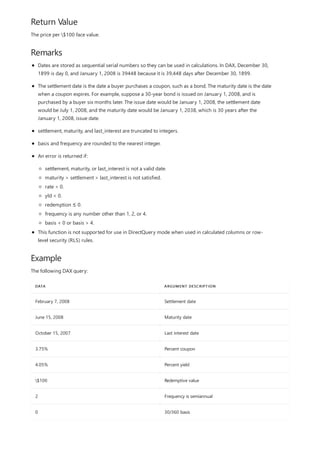
![EVALUATE
{
ODDLPRICE(DATE(2008,2,7), DATE(2008,6,15), DATE(2007,10,15), 0.0375, 0.0405, 100, 2, 0)
}
[VALUE]
99.8782860147213
Returns the price per $100 face value of a security that has an odd (short or long) last coupon period, using the
terms specified above.](https://image.slidesharecdn.com/funcoesdax-220812141017-bb6cd4dc/85/Funcoes-DAX-pdf-242-320.jpg)
![ODDLYIELD
11/30/2021 • 2 minutes to read
Syntax
ODDLYIELD(<settlement>, <maturity>, <last_interest>, <rate>, <pr>, <redemption>, <frequency>[, <basis>])
Parameters
TERM DEFINITION
settlement The security's settlement date. The security settlement date
is the date after the issue date when the security is traded to
the buyer.
maturity The security's maturity date. The maturity date is the date
when the security expires.
last_interest The security's last coupon date.
rate The security's interest rate.
pr The security's price.
redemption The security's redemption value per $100 face value.
frequency The number of coupon payments per year. For annual
payments, frequency = 1; for semiannual, frequency = 2; for
quarterly, frequency = 4.
basis (Optional) The type of day count basis to use. If basis is
omitted, it is assumed to be 0. The accepted values are listed
below this table.
BASIS DAY COUNT BASIS
0 or omitted US (NASD) 30/360
1 Actual/actual
2 Actual/360
3 Actual/365
4 European 30/360
Returns the yield of a security that has an odd (short or long) last period.
The basis parameter accepts the following values:](https://image.slidesharecdn.com/funcoesdax-220812141017-bb6cd4dc/85/Funcoes-DAX-pdf-243-320.jpg)
![Return Value
Remarks
Example
The security's yield.
Dates are stored as sequential serial numbers so they can be used in calculations. In DAX, December 30,
1899 is day 0, and January 1, 2008 is 39448 because it is 39,448 days after December 30, 1899.
The settlement date is the date a buyer purchases a coupon, such as a bond. The maturity date is the date
when a coupon expires. For example, suppose a 30-year bond is issued on January 1, 2008, and is
purchased by a buyer six months later. The issue date would be January 1, 2008, the settlement date
would be July 1, 2008, and the maturity date would be January 1, 2038, which is 30 years after the
January 1, 2008, issue date.
ODDLYIELD is calculated as follows:
$$text{ODDLYIELD} = bigg[ frac{(text{redemption} + ((sum^{text{NC}}_{i=1} frac{text{DC}_{i}}
{text{NL}_{i}}) times frac{100 times text{rate}}{text{frequency}})) - (text{par} +
((sum^{text{NC}}_{i=1} frac{text{A}_{i}}{text{NL}_{i}}) times frac{100 times text{rate}}
{text{frequency}}))}{text{par} + ((sum^{text{NC}}_{i=1} frac{text{A}_{i}}{text{NL}_{i}}) times frac{100
times text{rate}}{text{frequency}})} bigg] times bigg[ frac{text{frequency}}{(sum^{text{NC}}_{i=1}
frac{text{DSC}_{i}}{text{NL}_{i}})} bigg]$$
where:
$text{A}_{i}$ = number of accrued days for the $i^{th}$, or last, quasi-coupon period within odd
period counting forward from last interest date before redemption.
$text{DC}_{i}$ = number of days counted in the $i^{th}$, or last, quasi-coupon period as delimited by
the length of the actual coupon period.
$text{NC}$ = number of quasi-coupon periods that fit in odd period; if this number contains a
fraction it will be raised to the next whole number.
$text{NL}_{i}$ = normal length in days of the $i^{th}$, or last, quasi-coupon period within odd
coupon period.
settlement, maturity, last_interest are truncated to integers.
basis and frequency are rounded to the nearest integer.
An error is returned if:
settlement, maturity, last_interest is not a valid date.
maturity > settlement > last_interest is not satisfied.
rate < 0.
pr ≤ 0.
redemption ≤ 0.
frequency is any number other than 1, 2, or 4.
basis < 0 or basis > 4.
This function is not supported for use in DirectQuery mode when used in calculated columns or row-
level security (RLS) rules.
The following DAX query:](https://image.slidesharecdn.com/funcoesdax-220812141017-bb6cd4dc/85/Funcoes-DAX-pdf-244-320.jpg)
![DATA ARGUMENT DESCRIPTION
4/20/2008 Settlement date
6/15/2008 Maturity date
12/24/2007 Last interest date
3.75% Percent coupon
$99.875 Price
$100 Redemption value
2 Frequency is semiannual
0 30/360 basis
EVALUATE
{
ODDLYIELD(DATE(2008,4,20), DATE(2008,6,15), DATE(2007,12,24), 0.0375, 99.875, 100, 2, 0)
}
[VALUE]
0.0451922356291692
Returns the yield of a security that has an odd (short of long) last period, using the terms specified above.](https://image.slidesharecdn.com/funcoesdax-220812141017-bb6cd4dc/85/Funcoes-DAX-pdf-245-320.jpg)

![[VALUE]
3.85986616262266
Example 2
EVALUATE
{
PDURATION(0.025/12, 1000, 1200)
}
[VALUE]
87.6054764193714
The following DAX query:
Returns the number of months required for an investment of $1000, earning 2.5% annually, to reach $1200.](https://image.slidesharecdn.com/funcoesdax-220812141017-bb6cd4dc/85/Funcoes-DAX-pdf-247-320.jpg)
![PMT
11/30/2021 • 2 minutes to read
Syntax
PMT(<rate>, <nper>, <pv>[, <fv>[, <type>]])
Parameters
TERM DEFINITION
rate The interest rate for the loan.
nper The total number of payments for the loan.
pv The present value, or the total amount that a series of future
payments is worth now; also known as the principal.
fv (Optional) The future value, or a cash balance you want to
attain after the last payment is made. If fv is omitted, it is
assumed to be BLANK.
type (Optional) The number 0 or 1 which indicates when
payments are due. If type is omitted, it is assumed to be 0.
The accepted values are listed below this table.
SET TYPE EQUAL TO IF PAYMENTS ARE DUE
0 or omitted At the end of the period
1 At the beginning of the period
Return Value
Remarks
Calculates the payment for a loan based on constant payments and a constant interest rate.
The type parameter accepts the following values:
Note: For a more complete description of the arguments in PMT, see the PV function.
The amount of a single loan payment.
The payment returned by PMT includes principal and interest but no taxes, reserve payments, or fees
sometimes associated with loans.
Make sure that you are consistent about the units you use for specifying rate and nper. If you make
monthly payments on a four-year loan at an annual interest rate of 12 percent, use 0.12/12 for rate and
4*12 for nper. If you make annual payments on the same loan, use 0.12 for rate and 4 for nper.](https://image.slidesharecdn.com/funcoesdax-220812141017-bb6cd4dc/85/Funcoes-DAX-pdf-248-320.jpg)
![Examples
Example 1
DATA DESCRIPTION
8% Annual interest rate
10 Number of months of payments
$10,000 Amount of loan
EVALUATE
{
PMT(0.08/12, 10, 10000, 0, 1)
}
[VALUE]
-1030.16432717797
Example 2
DATA DESCRIPTION
6% Annual interest rate
18 Number of years of payments
$50,000 Amount of loan
type is rounded to the nearest integer.
An error is returned if:
nper < 1
Tip: To find the total amount paid over the duration of the loan, multiply the returned PMT value by nper.
This function is not supported for use in DirectQuery mode when used in calculated columns or row-level
security (RLS) rules.
The following DAX query:
Returns the monthly payment amount, paid at the beginning of the month, for a loan with the terms specified
above.
Note: 1030.16432717797 is the payment per period. As a result, the total amount paid over the duration of the
loan is approximately 1030.16 * 10 = $10,301.60. In other words, approximately $301.60 of interest is paid.
The following DAX query:](https://image.slidesharecdn.com/funcoesdax-220812141017-bb6cd4dc/85/Funcoes-DAX-pdf-249-320.jpg)
![EVALUATE
{
PMT(0.06/12, 18*12, 0, 50000)
}
[VALUE]
-129.081160867991
Returns the amount to save each month to have $50,000 at the end of 18 years, using the terms specified
above.](https://image.slidesharecdn.com/funcoesdax-220812141017-bb6cd4dc/85/Funcoes-DAX-pdf-250-320.jpg)
![PPMT
11/30/2021 • 2 minutes to read
Syntax
PPMT(<rate>, <per>, <nper>, <pv>[, <fv>[, <type>]])
Parameters
TERM DEFINITION
rate The interest rate for the loan.
per Specifies the period. Must be between 1 and nper (inclusive).
nper The total number of payment periods in an annuity.
pv The present value — the total amount that a series of future
payments is worth now.
fv (Optional) The future value, or a cash balance you want to
attain after the last payment is made. If fv is omitted, it is
assumed to be BLANK.
type (Optional) The number 0 or 1 which indicates when
payments are due. If type is omitted, it is assumed to be 0.
The accepted values are listed below this table.
SET TYPE EQUAL TO IF PAYMENTS ARE DUE
0 or omitted At the end of the period
1 At the beginning of the period
Return Value
Remarks
Returns the payment on the principal for a given period for an investment based on periodic, constant payments
and a constant interest rate.
The type parameter accepts the following values:
Note: For a more complete description of the arguments in PPMT, see the PV function.
The payment on the principal for a given period.
Make sure that you are consistent about the units you use for specifying rate and nper. If you make
monthly payments on a four-year loan at an annual interest rate of 12 percent, use 0.12/12 for rate and
4*12 for nper. If you make annual payments on the same loan, use 0.12 for rate and 4 for nper.](https://image.slidesharecdn.com/funcoesdax-220812141017-bb6cd4dc/85/Funcoes-DAX-pdf-251-320.jpg)
![Example 1
DATA ARGUMENT DESCRIPTION
10% Annual interest rate
2 Number of years for the loan
$2,000.00 Amount of loan
EVALUATE
{
PPMT(0.1/12, 1, 2*12, 2000.00)
}
[VALUE]
-75.6231860083663
Example 2
DATA ARGUMENT DESCRIPTION
8% Annual interest rate
10 Number of years for the loan
$200,000.00 Amount of loan
EVALUATE
{
PPMT(0.08, 10, 10, 200000.00)
}
type is rounded to the nearest integer.
An error is returned if:
per < 1 or per > nper
nper < 1
This function is not supported for use in DirectQuery mode when used in calculated columns or row-
level security (RLS) rules.
The following DAX query:
Returns the principal payment made in the first month for a loan with the terms specified above.
The following DAX query:
Returns the principal payment made in the 10th year for a loan with the terms specified above.](https://image.slidesharecdn.com/funcoesdax-220812141017-bb6cd4dc/85/Funcoes-DAX-pdf-252-320.jpg)
![[VALUE]
-27598.0534624214](https://image.slidesharecdn.com/funcoesdax-220812141017-bb6cd4dc/85/Funcoes-DAX-pdf-253-320.jpg)
![PRICE
11/30/2021 • 2 minutes to read
Syntax
PRICE(<settlement>, <maturity>, <rate>, <yld>, <redemption>, <frequency>[, <basis>])
Parameters
TERM DEFINITION
settlement The security's settlement date. The security settlement date
is the date after the issue date when the security is traded to
the buyer.
maturity The security's maturity date. The maturity date is the date
when the security expires.
rate The security's annual coupon rate.
yld The security's annual yield.
redemption The security's redemption value per $100 face value.
frequency The number of coupon payments per year. For annual
payments, frequency = 1; for semiannual, frequency = 2; for
quarterly, frequency = 4.
basis (Optional) The type of day count basis to use. If basis is
omitted, it is assumed to be 0. The accepted values are listed
below this table.
BASIS DAY COUNT BASIS
0 or omitted US (NASD) 30/360
1 Actual/actual
2 Actual/360
3 Actual/365
4 European 30/360
Return Value
Returns the price per $100 face value of a security that pays periodic interest.
The basis parameter accepts the following values:](https://image.slidesharecdn.com/funcoesdax-220812141017-bb6cd4dc/85/Funcoes-DAX-pdf-254-320.jpg)
![Remarks
The price per $100 face value.
Dates are stored as sequential serial numbers so they can be used in calculations. In DAX, December 30,
1899 is day 0, and January 1, 2008 is 39448 because it is 39,448 days after December 30, 1899.
The settlement date is the date a buyer purchases a coupon, such as a bond. The maturity date is the date
when a coupon expires. For example, suppose a 30-year bond is issued on January 1, 2008, and is
purchased by a buyer six months later. The issue date would be January 1, 2008, the settlement date
would be July 1, 2008, and the maturity date would be January 1, 2038, which is 30 years after the
January 1, 2008, issue date.
settlement and maturity are truncated to integers.
basis and frequency are rounded to the nearest integer.
An error is returned if:
settlement or maturity is not a valid date.
settlement ≥ maturity.
rate < 0.
yld < 0.
redemption ≤ 0.
frequency is any number other than 1, 2, or 4.
basis < 0 or basis > 4.
This function is not supported for use in DirectQuery mode when used in calculated columns or row-
level security (RLS) rules.
Important:
When N > 1 (N is the number of coupons payable between the settlement date and redemption
date), PRICE is calculated as follows:
$$text{PRICE} = bigg[ frac{text{redemption}}{(1 + frac{text{yld}}{text{frequency}})^{(N - 1 +
frac{text{DSC}}{text{E}})})} bigg] + bigg[ sum^{N}_{k=1} frac{100 times frac{text{rate}}
{text{frequency}}}{(1 + frac{text{yld}}{text{frequency}})^{(k - 1 + frac{text{DSC}}{text{E}})}} bigg] -
bigg[ 100 times frac{text{rate}}{text{frequency}} times frac{text{A}}{text{E}} bigg]$$
When N = 1 (N is the number of coupons payable between the settlement date and redemption
date), PRICE is calculated as follows:
$$text{DSR} = text{E} - text{A}$$
$$text{T1} = 100 times frac{text{rate}}{text{frequency}} + text{redemption}$$
$$text{T2} = frac{text{yld}}{text{frequency}} times frac{text{DSR}}{text{E}} + 1$$
$$text{T3} = 100 times frac{text{rate}}{text{frequency}} times frac{text{A}}{text{E}}$$
$$text{PRICE} = frac{text{T1}}{text{T2}} - text{T3}$$
where:
$text{DSC}$ = number of days from settlement to next coupon date.
$text{E}$ = number of days in coupon period in which the settlement date falls.
$text{A}$ = number of days from beginning of coupon period to settlement date.](https://image.slidesharecdn.com/funcoesdax-220812141017-bb6cd4dc/85/Funcoes-DAX-pdf-255-320.jpg)
![Example
DATA ARGUMENT DESCRIPTION
2/15/2008 Settlement date
11/15/2017 Maturity date
5.75% Percent semiannual coupon
6.50% Percent yield
$100 Redemption value
2 Frequency is semiannual
0 30/360 basis
EVALUATE
{
PRICE(DATE(2008,2,15), DATE(2017,11,15), 0.0575, 0.065, 100, 2, 0)
}
[VALUE]
94.6343616213221
The following DAX query:
Returns the bond price, for a bond using the terms specified above.](https://image.slidesharecdn.com/funcoesdax-220812141017-bb6cd4dc/85/Funcoes-DAX-pdf-256-320.jpg)
![PRICEDISC
11/30/2021 • 2 minutes to read
Syntax
PRICEDISC(<settlement>, <maturity>, <discount>, <redemption>[, <basis>])
Parameters
TERM DEFINITION
settlement The security's settlement date. The security settlement date
is the date after the issue date when the security is traded to
the buyer.
maturity The security's maturity date. The maturity date is the date
when the security expires.
discount The security's discount rate.
redemption The security's redemption value per $100 face value.
basis (Optional) The type of day count basis to use. If basis is
omitted, it is assumed to be 0. The accepted values are listed
below this table.
BASIS DAY COUNT BASIS
0 or omitted US (NASD) 30/360
1 Actual/actual
2 Actual/360
3 Actual/365
4 European 30/360
Return Value
Remarks
Returns the price per $100 face value of a discounted security.
The basis parameter accepts the following values:
The price per $100 face value.
Dates are stored as sequential serial numbers so they can be used in calculations. In DAX, December 30,
1899 is day 0, and January 1, 2008 is 39448 because it is 39,448 days after December 30, 1899.](https://image.slidesharecdn.com/funcoesdax-220812141017-bb6cd4dc/85/Funcoes-DAX-pdf-257-320.jpg)
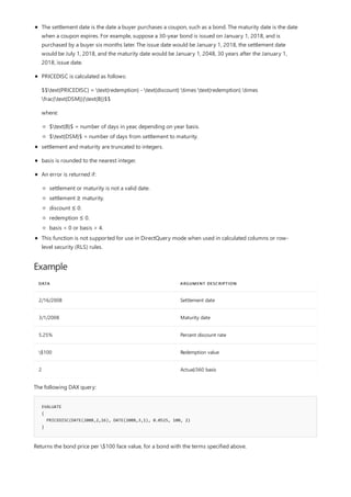
![[VALUE]
99.7958333333333](https://image.slidesharecdn.com/funcoesdax-220812141017-bb6cd4dc/85/Funcoes-DAX-pdf-259-320.jpg)
![PRICEMAT
11/30/2021 • 2 minutes to read
Syntax
PRICEMAT(<settlement>, <maturity>, <issue>, <rate>, <yld>[, <basis>])
Parameters
TERM DEFINITION
settlement The security's settlement date. The security settlement date
is the date after the issue date when the security is traded to
the buyer.
maturity The security's maturity date. The maturity date is the date
when the security expires.
issue The security's issue date.
rate The security's interest rate at date of issue.
yld The security's annual yield.
basis (Optional) The type of day count basis to use. If basis is
omitted, it is assumed to be 0. The accepted values are listed
below this table.
BASIS DAY COUNT BASIS
0 or omitted US (NASD) 30/360
1 Actual/actual
2 Actual/360
3 Actual/365
4 European 30/360
Return Value
Remarks
Returns the price per $100 face value of a security that pays interest at maturity.
The basis parameter accepts the following values:
The price per $100 face value.](https://image.slidesharecdn.com/funcoesdax-220812141017-bb6cd4dc/85/Funcoes-DAX-pdf-260-320.jpg)
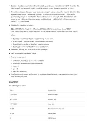
![EVALUATE
{
PRICEMAT(DATE(2008,2,15), DATE(2008,4,13), DATE(2007,11,11), 0.061, 0.061, 0)
}
[VALUE]
99.9844988755569
Returns the price per $100 face value of a security with the terms specified above.](https://image.slidesharecdn.com/funcoesdax-220812141017-bb6cd4dc/85/Funcoes-DAX-pdf-262-320.jpg)
![PV
11/30/2021 • 3 minutes to read
Syntax
PV(<rate>, <nper>, <pmt>[, <fv>[, <type>]])
Parameters
TERM DEFINITION
rate The interest rate per period. For example, if you obtain an
automobile loan at a 10 percent annual interest rate and
make monthly payments, your interest rate per month is
0.1/12, or 0.0083. You would enter 0.1/12, or 0.0083, into
the formula as the rate.
nper The total number of payment periods in an annuity. For
example, if you get a four-year car loan and make monthly
payments, your loan has 4*12 (or 48) periods. You would
enter 48 into the formula for nper.
pmt The payment made each period that cannot change over the
life of the annuity. Typically, pmt includes principal and
interest but no other fees or taxes. For example, the monthly
payments on a $10,000, four-year car loan at 12 percent
are $263.33. You would enter -263.33 into the formula as
the pmt.
fv (Optional) The future value, or a cash balance you want to
attain after the last payment is made. If fv is omitted, it is
assumed to be BLANK. For example, if you want to save
$50,000 to pay for a special project in 18 years, then
$50,000 is the future value. You could then make a
conservative guess at an interest rate and determine how
much you must save each month.
type (Optional) The number 0 or 1 which indicates when
payments are due. If type is omitted, it is assumed to be 0.
The accepted values are listed below this table.
SET TYPE EQUAL TO IF PAYMENTS ARE DUE
0 or omitted At the end of the period
1 At the beginning of the period
Calculates the present value of a loan or an investment, based on a constant interest rate. You can use PV with
either periodic, constant payments (such as a mortgage or other loan), and/or a future value that's your
investment goal.
The type parameter accepts the following values:](https://image.slidesharecdn.com/funcoesdax-220812141017-bb6cd4dc/85/Funcoes-DAX-pdf-263-320.jpg)
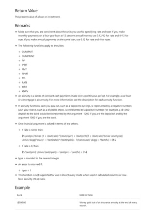
![8% Interest rate earned on the money paid out.
20 Years the money will be paid out.
DATA DESCRIPTION
EVALUATE
{
PV(0.08/12, 12*20, 500.00, 0, 0)
}
[VALUE]
-59777.1458511878
The following DAX query:
Returns the present value of an annuity using the terms specified above.](https://image.slidesharecdn.com/funcoesdax-220812141017-bb6cd4dc/85/Funcoes-DAX-pdf-265-320.jpg)
![RATE
11/30/2021 • 2 minutes to read
Syntax
RATE(<nper>, <pmt>, <pv>[, <fv>[, <type>[, <guess>]]])
Parameters
TERM DEFINITION
nper The total number of payment periods in an annuity.
pmt The payment made each period and cannot change over the
life of the annuity. Typically, pmt includes principal and
interest but no other fees or taxes.
pv The present value — the total amount that a series of future
payments is worth now.
fv (Optional) The future value, or a cash balance you want to
attain after the last payment is made. If fv is omitted, it is
assumed to be 0 (the future value of a loan, for example, is
0).
type (Optional) The number 0 or 1 which indicates when
payments are due. If type is omitted, it is assumed to be 0.
The accepted values are listed below this table.
guess (Optional) Your guess for what the rate will be.
- If omitted, it is assumed to be 10%.
- If RATE does not converge, try different values for guess.
RATE usually converges if guess is between 0 and 1.
SET TYPE EQUAL TO IF PAYMENTS ARE DUE
0 or omitted At the end of the period
1 At the beginning of the period
Return Value
Returns the interest rate per period of an annuity. RATE is calculated by iteration and can have zero or more
solutions. If the successive results of RATE do not converge to within 0.0000001 after 20 iterations, an error is
returned.
The type parameter accepts the following values:
The interest rate per period.](https://image.slidesharecdn.com/funcoesdax-220812141017-bb6cd4dc/85/Funcoes-DAX-pdf-266-320.jpg)
![Remarks
Examples
DATA DESCRIPTION
4 Years of the loan
-200 Monthly payment
8000 Amount of the loan
Example 1
EVALUATE
{
RATE(4*12, -200, 8000)
}
[VALUE]
0.00770147248820137
Example 2
EVALUATE
{
RATE(4*12, -200, 8000) * 12
}
[VALUE]
0.0924176698584164
Make sure that you are consistent about the units you use for specifying guess and nper. If you make
monthly payments on a four-year loan at 12 percent annual interest, use 0.12/12 for guess and 4*12 for
nper. If you make annual payments on the same loan, use 0.12 for guess and 4 for nper.
type is rounded to the nearest integer.
An error is returned if:
nper ≤ 0.
RATE does not converge to within 0.0000001 after 20 iterations
This function is not supported for use in DirectQuery mode when used in calculated columns or row-
level security (RLS) rules.
The following DAX query:
Returns the monthly rate of the loan using the terms specified above.
The following DAX query:
Returns the annual rate of the loan using the terms specified above.](https://image.slidesharecdn.com/funcoesdax-220812141017-bb6cd4dc/85/Funcoes-DAX-pdf-267-320.jpg)
![RECEIVED
11/30/2021 • 2 minutes to read
Syntax
RECEIVED(<settlement>, <maturity>, <investment>, <discount>[, <basis>])
Parameters
TERM DEFINITION
settlement The security's settlement date. The security settlement date
is the date after the issue date when the security is traded to
the buyer.
maturity The security's maturity date. The maturity date is the date
when the security expires.
investment The amount invested in the security.
discount The security's discount rate.
basis (Optional) The type of day count basis to use. If basis is
omitted, it is assumed to be 0. The accepted values are listed
below this table.
BASIS DAY COUNT BASIS
0 or omitted US (NASD) 30/360
1 Actual/actual
2 Actual/360
3 Actual/365
4 European 30/360
Return Value
Remarks
Returns the amount received at maturity for a fully invested security.
The basis parameter accepts the following values:
The amount received at maturity.
Dates are stored as sequential serial numbers so they can be used in calculations. In DAX, December 30,
1899 is day 0, and January 1, 2008 is 39448 because it is 39,448 days after December 30, 1899.](https://image.slidesharecdn.com/funcoesdax-220812141017-bb6cd4dc/85/Funcoes-DAX-pdf-268-320.jpg)
![Example
DATA DESCRIPTION
15-Feb-08 Settlement (issue) date
15-May-08 Maturity date
$1,000,000.00 Investment
5.75% Percent discount rate
2 Actual/360 basis
EVALUATE
{
RECEIVED(DATE(2008,2,15), DATE(2008,5,15), 1000000.00, 0.0575, 2)
}
[VALUE]
1014584.6544071
The settlement date is the date a buyer purchases a coupon, such as a bond. The maturity date is the date
when a coupon expires. For example, suppose a 30-year bond is issued on January 1, 2008, and is
purchased by a buyer six months later. The issue date would be January 1, 2008, the settlement date
would be July 1, 2008, and the maturity date would be January 1, 2038, which is 30 years after the
January 1, 2008, issue date.
RECEIVED is calculated as follows:
$$text{RECEIVED} = frac{text{investment}}{1 - (text{discount} times frac{text{DIM}}{text{B}})}$$
where:
$text{B}$ = number of days in a year, depending on the year basis.
$text{DIM}$ = number of days from issue to maturity.
settlement and maturity are truncated to integers.
basis is rounded to the nearest integer.
An error is returned if:
settlement or maturity is not a valid date.
settlement ≥ maturity.
investment ≤ 0.
discount ≤ 0.
basis < 0 or basis > 4.
This function is not supported for use in DirectQuery mode when used in calculated columns or row-
level security (RLS) rules.
The following DAX query:
Returns the total amount to be received at maturity, for a bond with the terms specified above.](https://image.slidesharecdn.com/funcoesdax-220812141017-bb6cd4dc/85/Funcoes-DAX-pdf-269-320.jpg)
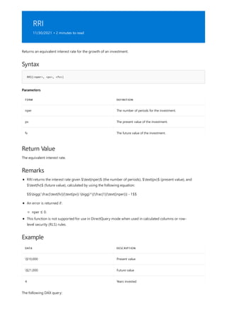
![EVALUATE
{
RRI(4*12, 10000, 21000)
}
[VALUE]
0.0155771057566627
Returns an equivalent interest rate for the growth of an investment with the terms specified above.](https://image.slidesharecdn.com/funcoesdax-220812141017-bb6cd4dc/85/Funcoes-DAX-pdf-271-320.jpg)
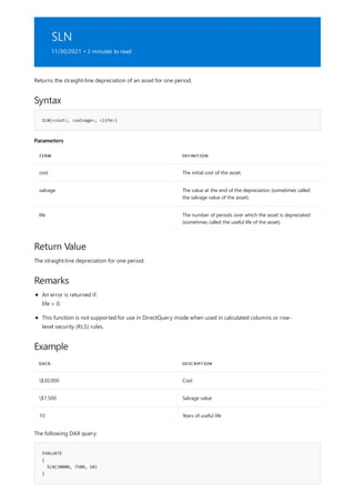
![[VALUE]
2250
Returns the yearly depreciation allowance using the terms specified above.](https://image.slidesharecdn.com/funcoesdax-220812141017-bb6cd4dc/85/Funcoes-DAX-pdf-273-320.jpg)
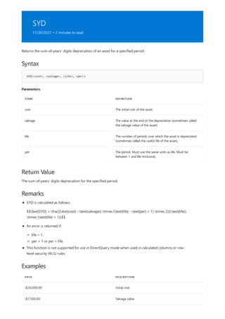
![10 Lifespan in years
DATA DESCRIPTION
Example 1
EVALUATE
{
SYD(30000.00, 7500.00, 10, 1)
}
[VALUE]
4090.90909090909
Example 2
EVALUATE
{
SYD(30000.00, 7500.00, 10, 10)
}
[VALUE]
409.090909090909
The following DAX query:
Returns an asset's sum-of-years' digits depreciation allowance for the first year, given the terms specified above.
The following DAX query:
Returns an asset's sum-of-years' digits depreciation allowance for the tenth (final) year, given the terms specified
above.](https://image.slidesharecdn.com/funcoesdax-220812141017-bb6cd4dc/85/Funcoes-DAX-pdf-275-320.jpg)

![DATA DESCRIPTION
3/31/2008 Settlement date
6/1/2008 Maturity date
9.14% Percent discount rate
EVALUATE
{
TBILLEQ(DATE(2008,3,31), DATE(2008,6,1), 0.0914)
}
[VALUE]
0.094151493565943
The following DAX query:
Returns the bond-equivalent yield for a Treasury bill using the terms specified above.](https://image.slidesharecdn.com/funcoesdax-220812141017-bb6cd4dc/85/Funcoes-DAX-pdf-277-320.jpg)
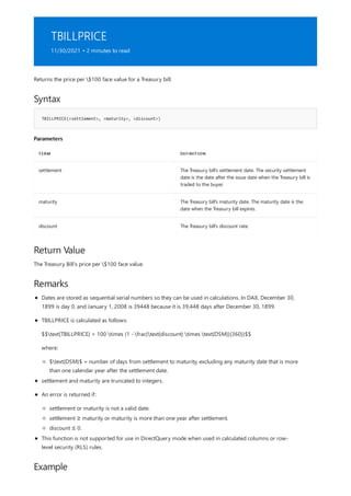
![DATA DESCRIPTION
3/31/2008 Settlement date
6/1/2008 Maturity date
9.0% Percent discount rate
EVALUATE
{
TBILLPRICE(DATE(2008,3,31), DATE(2008,6,1), 0.09)
}
[VALUE]
98.45
The following DAX query:
Returns the Treasury Bill's price per $100 face value, given the terms specified above.](https://image.slidesharecdn.com/funcoesdax-220812141017-bb6cd4dc/85/Funcoes-DAX-pdf-279-320.jpg)

![DATA DESCRIPTION
3/31/2008 Settlement date
6/1/2008 Maturity date
$98.45 Price per $100 face value
EVALUATE
{
TBILLYIELD(DATE(2008,3,31), DATE(2008,6,1), 98.45)
}
[VALUE]
0.0914169629253426
The following DAX query:
Returns the yield of a Treasury bill using the terms specified above.](https://image.slidesharecdn.com/funcoesdax-220812141017-bb6cd4dc/85/Funcoes-DAX-pdf-281-320.jpg)
![VDB
11/30/2021 • 2 minutes to read
Syntax
VDB(<cost>, <salvage>, <life>, <start_period>, <end_period>[, <factor>[, <no_switch>]])
Parameters
TERM DEFINITION
cost The initial cost of the asset.
salvage The value at the end of the depreciation (sometimes called
the salvage value of the asset). This value can be 0.
life The number of periods over which the asset is being
depreciated (sometimes called the useful life of the asset).
start_period The starting period for which you want to calculate the
depreciation. Start_period must use the same units as life.
Must be between 1 and life (inclusive).
end_period The ending period for which you want to calculate the
depreciation. End_period must use the same units as life.
Must be between start_period and life (inclusive).
factor (Optional) The rate at which the balance declines. If factor is
omitted, it is assumed to be 2 (the double-declining balance
method). Change factor if you do not want to use the
double-declining balance method. For a description of the
double-declining balance method, see DDB.
no_switch (Optional) A logical value specifying whether to switch to
straight-line depreciation when depreciation is greater than
the declining balance calculation. If omitted, it is assumed to
be FALSE.
- If no_switch evaluates to TRUE, VDB does not switch to
straight-line depreciation, even when the depreciation is
greater than the declining balance calculation.
- If no_switch evaluates to FALSE or is omitted, VDB switches
to straight-line depreciation when depreciation is greater
than the declining balance calculation.
Return Value
Returns the depreciation of an asset for any period you specify, including partial periods, using the double-
declining balance method or some other method you specify. VDB stands for variable declining balance.
The depreciation over the specified period.](https://image.slidesharecdn.com/funcoesdax-220812141017-bb6cd4dc/85/Funcoes-DAX-pdf-282-320.jpg)
![Remarks
Examples
DATA DESCRIPTION
2400 Initial cost
300 Salvage value
10 Lifetime in years
Example 1
EVALUATE
{
VDB(2400, 300, 10*365, 0, 1)
}
[VALUE]
1.31506849315068
Example 2
EVALUATE
{
VDB(2400, 300, 10*12, 6, 18, 3)
}
[VALUE]
540.185558199698
An error is returned if:
cost < 0.
salvage < 0.
life < 1.
start_period < 1 or start_period > end_period.
end_period < start_period or end_period > life.
factor < 0.
no_switch does not evaluate to either TRUE or FALSE.
This function is not supported for use in DirectQuery mode when used in calculated columns or row-
level security (RLS) rules.
The following DAX query:
Returns an asset's first day's depreciation using a factor of 2.
The following DAX query:
Returns an asset's depreciation between the 6$^{th}$ month and the 18$^{th}$ month. This calculation uses a
factor of 3.](https://image.slidesharecdn.com/funcoesdax-220812141017-bb6cd4dc/85/Funcoes-DAX-pdf-283-320.jpg)
![Example 3
EVALUATE
{
VDB(2400, 300, 10, 0, 0.875, 1.5)
}
[VALUE]
315
The following DAX query:
Returns an asset's depreciation in the first fiscal year that you own it, assuming that tax laws limit you to 150%
depreciation of the declining balance. The asset is purchased in the middle of the first quarter of the fiscal year.](https://image.slidesharecdn.com/funcoesdax-220812141017-bb6cd4dc/85/Funcoes-DAX-pdf-284-320.jpg)
![XIRR
11/30/2021 • 2 minutes to read
Syntax
XIRR(<table>, <values>, <dates>, [, <guess>[, <alternateResult>]])
Parameters
TERM DEFINITION
table A table for which the values and dates expressions should be
calculated.
values An expression that returns the cash flow value for each row
of the table.
dates An expression that returns the cash flow date for each row
of the table.
guess (Optional) An initial guess for the internal rate of return. If
omitted, the default guess of 0.1 is used.
alternateResult (Optional) A value returned in place of an error when a
solution cannot be determined.
Return value
Remarks
Returns the internal rate of return for a schedule of cash flows that is not necessarily periodic.
Internal rate of return for the given inputs. If the calculation fails to return a valid result, an error or value
specified as alternateResult is returned.
The value is calculated as the rate that satisfies the following function:
$$sum^{N}_{j=1} frac{P_{j}}{(1 + text{rate})^{frac{d_{j} - d_{1}}{365}}}$$
Where:
$P_{j}$ is the $j^{th}$ payment
$d_{j}$ is the $j^{th}$ payment date
$d_{1}$ is the first payment date
The series of cash flow values must contain at least one positive number and one negative number.
Avoid using ISERROR or IFERROR functions to capture an error returned by XIRR. If some inputs to the
function may result in a no solution error, providing an alternateResult parameter is the most reliable and
highest performing way to handle the error.
This function is not supported for use in DirectQuery mode when used in calculated columns or row-](https://image.slidesharecdn.com/funcoesdax-220812141017-bb6cd4dc/85/Funcoes-DAX-pdf-285-320.jpg)
![Example
= XIRR( CashFlows, [Payment], [Date] )
DATE PAYMENT
1/1/2014 -10000
3/1/2014 2750
10/30/2014 4250
2/15/2015 3250
4/1/2015 2750
level security (RLS) rules.
The following formula calculates the internal rate of return of the CashFlows table:
Rate of return = 37.49%](https://image.slidesharecdn.com/funcoesdax-220812141017-bb6cd4dc/85/Funcoes-DAX-pdf-286-320.jpg)
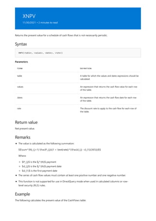
![= XNPV( CashFlows, [Payment], [Date], 0.09 )
DATE PAYMENT
1/1/2014 -10000
3/1/2014 2750
10/30/2014 4250
2/15/2015 3250
4/1/2015 2750
Present value = 2086.65](https://image.slidesharecdn.com/funcoesdax-220812141017-bb6cd4dc/85/Funcoes-DAX-pdf-288-320.jpg)
![YIELD
11/30/2021 • 2 minutes to read
Syntax
YIELD(<settlement>, <maturity>, <rate>, <pr>, <redemption>, <frequency>[, <basis>])
Parameters
TERM DEFINITION
settlement The security's settlement date. The security settlement date
is the date after the issue date when the security is traded to
the buyer.
maturity The security's maturity date. The maturity date is the date
when the security expires.
rate The security's annual coupon rate.
pr The security's price per $100 face value.
redemption The security's redemption value per $100 face value.
frequency The number of coupon payments per year. For annual
payments, frequency = 1; for semiannual, frequency = 2; for
quarterly, frequency = 4.
basis (Optional) The type of day count basis to use. If basis is
omitted, it is assumed to be 0. The accepted values are listed
below this table.
BASIS DAY COUNT BASIS
0 or omitted US (NASD) 30/360
1 Actual/actual
2 Actual/360
3 Actual/365
4 European 30/360
Return Value
Returns the yield on a security that pays periodic interest. Use YIELD to calculate bond yield.
The basis parameter accepts the following values:](https://image.slidesharecdn.com/funcoesdax-220812141017-bb6cd4dc/85/Funcoes-DAX-pdf-289-320.jpg)
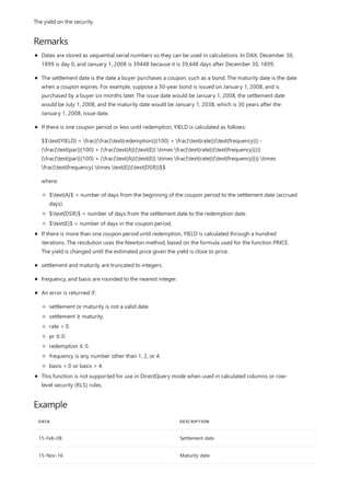
![5.75% Percent coupon
95.04287 Price
$100 Redemption value
2 Frequency is semiannual (see above)
0 30/360 basis (see above)
DATA DESCRIPTION
EVALUATE
{
YIELD(DATE(2008,2,15), DATE(2016,11,15), 0.0575, 95.04287, 100, 2,0)
}
[VALUE]
0.0650000068807314
The following DAX query:
Returns the yield on a bond with the terms specified above.](https://image.slidesharecdn.com/funcoesdax-220812141017-bb6cd4dc/85/Funcoes-DAX-pdf-291-320.jpg)
![YIELDDISC
11/30/2021 • 2 minutes to read
Syntax
YIELDDISC(<settlement>, <maturity>, <pr>, <redemption>[, <basis>])
Parameters
TERM DEFINITION
settlement The security's settlement date. The security settlement date
is the date after the issue date when the security is traded to
the buyer.
maturity The security's maturity date. The maturity date is the date
when the security expires.
pr The security's price per $100 face value.
redemption The security's redemption value per $100 face value.
basis (Optional) The type of day count basis to use. If basis is
omitted, it is assumed to be 0. The accepted values are listed
below this table.
BASIS DAY COUNT BASIS
0 or omitted US (NASD) 30/360
1 Actual/actual
2 Actual/360
3 Actual/365
4 European 30/360
Return Value
Remarks
Returns the annual yield for a discounted security.
The basis parameter accepts the following values:
The annual yield.
Dates are stored as sequential serial numbers so they can be used in calculations. In DAX, December 30,
1899 is day 0, and January 1, 2008 is 39448 because it is 39,448 days after December 30, 1899.](https://image.slidesharecdn.com/funcoesdax-220812141017-bb6cd4dc/85/Funcoes-DAX-pdf-292-320.jpg)
![Example
DATA -
16-Feb-08 Settlement date
1-Mar-08 Maturity date
99.795 Price
$100 Redemption value
2 Actual/360 basis
EVALUATE
{
YIELDDISC(DATE(2008,2,16), DATE(2008,3,1), 99.795, 100, 2)
}
[VALUE]
0.0528225719868583
The settlement date is the date a buyer purchases a coupon, such as a bond. The maturity date is the date
when a coupon expires. For example, suppose a 30-year bond is issued on January 1, 2008, and is
purchased by a buyer six months later. The issue date would be January 1, 2008, the settlement date
would be July 1, 2008, and the maturity date would be January 1, 2038, which is 30 years after the
January 1, 2008, issue date.
settlement and maturity are truncated to integers.
basis is rounded to the nearest integer.
An error is returned if:
settlement or maturity is not a valid date.
settlement ≥ maturity.
pr ≤ 0.
redemption ≤ 0.
basis < 0 or basis > 4.
This function is not supported for use in DirectQuery mode when used in calculated columns or row-
level security (RLS) rules.
The following DAX query:
Returns the security's annual yield, given the terms specified above.](https://image.slidesharecdn.com/funcoesdax-220812141017-bb6cd4dc/85/Funcoes-DAX-pdf-293-320.jpg)
![YIELDMAT
11/30/2021 • 2 minutes to read
Syntax
YIELDMAT(<settlement>, <maturity>, <issue>, <rate>, <pr>[, <basis>])
Parameters
TERM DEFINITION
settlement The security's settlement date. The security settlement date
is the date after the issue date when the security is traded to
the buyer.
maturity The security's maturity date. The maturity date is the date
when the security expires.
issue The security's issue date.
rate The security's interest rate at date of issue.
pr The security's price per $100 face value.
basis (Optional) The type of day count basis to use. If basis is
omitted, it is assumed to be 0. The accepted values are listed
below this table.
BASIS DAY COUNT BASIS
0 or omitted US (NASD) 30/360
1 Actual/actual
2 Actual/360
3 Actual/365
4 European 30/360
Return Value
Remarks
Returns the annual yield of a security that pays interest at maturity.
The basis parameter accepts the following values:
The annual yield.](https://image.slidesharecdn.com/funcoesdax-220812141017-bb6cd4dc/85/Funcoes-DAX-pdf-294-320.jpg)
![Example
DATA DESCRIPTION
15-Mar-08 Settlement date
3-Nov-08 Maturity date
8-Nov-07 Issue date
6.25% Percent semiannual coupon
100.0123 Price
0 30/360 basis (see above)
EVALUATE
{
YIELDMAT(DATE(2008,3,15), DATE(2008,11,3), DATE(2007,11,8), 0.0625, 100.0123, 0)
}
[VALUE]
0.0609543336915387
Dates are stored as sequential serial numbers so they can be used in calculations. In DAX, December 30,
1899 is day 0, and January 1, 2008 is 39448 because it is 39,448 days after December 30, 1899.
The settlement date is the date a buyer purchases a coupon, such as a bond. The maturity date is the date
when a coupon expires. For example, suppose a 30-year bond is issued on January 1, 2008, and is
purchased by a buyer six months later. The issue date would be January 1, 2008, the settlement date
would be July 1, 2008, and the maturity date would be January 1, 2038, which is 30 years after the
January 1, 2008, issue date.
settlement, maturity, and issue are truncated to integers.
basis is rounded to the nearest integer.
An error is returned if:
settlement, maturity, or issue is not a valid date.
maturity > settlement > issue is not satisfied.
rate < 0.
pr ≤ 0.
basis < 0 or basis > 4.
This function is not supported for use in DirectQuery mode when used in calculated columns or row-
level security (RLS) rules.
The following DAX query:
Returns the yield for a security using the terms specified above.](https://image.slidesharecdn.com/funcoesdax-220812141017-bb6cd4dc/85/Funcoes-DAX-pdf-295-320.jpg)
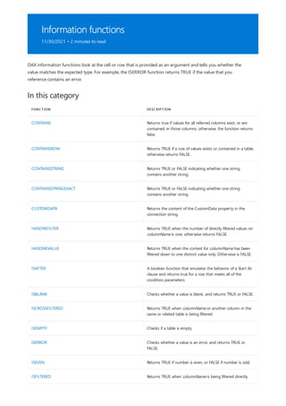
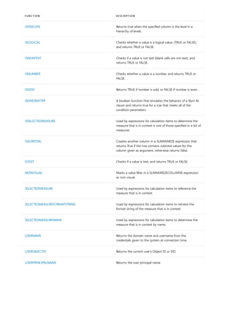
![CONTAINS
11/30/2021 • 2 minutes to read
Syntax
CONTAINS(<table>, <columnName>, <value>[, <columnName>, <value>]…)
Parameters
TERM DEFINITION
table Any DAX expression that returns a table of data.
columnName The name of an existing column, using standard DAX syntax.
It cannot be an expression.
value Any DAX expression that returns a single scalar value, that is
to be sought in columnName. The expression is to be
evaluated exactly once and before it is passed to the
argument list.
Return value
Remarks
Example
= CONTAINS(InternetSales, [ProductKey], 214, [CustomerKey], 11185)
Returns true if values for all referred columns exist, or are contained, in those columns; otherwise, the function
returns false.
A value of TRUE if each specified value can be found in the corresponding columnName, or are contained, in
those columns; otherwise, the function returns FALSE.
The arguments columnName and value must come in pairs; otherwise an error is returned.
columnName must belong to the specified table, or to a table that is related to table.
If columnName refers to a column in a related table then it must be fully qualified; otherwise, an error is
returned.
This function is not supported for use in DirectQuery mode when used in calculated columns or row-
level security (RLS) rules.
The following example creates a measure that tells you whether there were any Internet sales of product 214
and to customer 11185 at the same time.](https://image.slidesharecdn.com/funcoesdax-220812141017-bb6cd4dc/85/Funcoes-DAX-pdf-298-320.jpg)
![CONTAINSROW function
11/30/2021 • 2 minutes to read
Syntax
CONTAINSROW(<tableExpr>, <scalarExpr>[, <scalarExpr>, …])
Parameters
TERM DEFINITION
scalarExprN Any valid DAX expression that returns a scalar value.
tableExpr Any valid DAX expression that returns a table of data.
Return value
Remarks
Example 1
EVALUATE FILTER(ALL(DimProduct[Color]), [Color] IN { "Red", "Yellow", "Blue" })
ORDER BY [Color]
EVALUATE FILTER(ALL(DimProduct[Color]), ([Color]) IN { "Red", "Yellow", "Blue" })
ORDER BY [Color]
Returns TRUE if a row of values exists or contained in a table, otherwise returns FALSE.
TRUE or FALSE.
<scalarExpr> IN <tableExpr>
( <scalarExpr1>, <scalarExpr2>, … ) IN <tableExpr>
Except syntax, the IN operator and CONTAINSROW function are functionally equivalent.
The number of scalarExprN must match the number of columns in tableExpr.
NOT IN is not an operator in DAX. To perform the logical negation of the IN operator, put NOT in front
of the entire expression. For example, NOT [Color] IN { "Red", "Yellow", "Blue" }.
Unlike the = operator, the IN operator and the CONTAINSROW function perform strict comparison. For
example, the BLANK value does not match 0.
The following equivalent DAX queries:
and
and](https://image.slidesharecdn.com/funcoesdax-220812141017-bb6cd4dc/85/Funcoes-DAX-pdf-299-320.jpg)
![EVALUATE FILTER(ALL(DimProduct[Color]), CONTAINSROW({ "Red", "Yellow", "Blue" }, [Color]))
ORDER BY [Color]
DIMPRODUCT[COLOR]
Blue
Red
Yellow
Example 2
EVALUATE FILTER(SUMMARIZE(DimProduct, [Color], [Size]), ([Color], [Size]) IN { ("Black", "L") })
EVALUATE FILTER(SUMMARIZE(DimProduct, [Color], [Size]), CONTAINSROW({ ("Black", "L") }, [Color], [Size]))
DIMPRODUCT[COLOR] DIMPRODUCT[SIZE]
Black L
Example 3
EVALUATE FILTER(ALL(DimProduct[Color]), NOT [Color] IN { "Red", "Yellow", "Blue" })
ORDER BY [Color]
EVALUATE FILTER(ALL(DimProduct[Color]), NOT CONTAINSROW({ "Red", "Yellow", "Blue" }, [Color]))
ORDER BY [Color]
DIMPRODUCT[COLOR]
Black
Grey
Multi
Return the following table with a single column:
The following equivalent DAX queries:
and
Return:
The following equivalent DAX queries:
and
Return the following table with a single column:](https://image.slidesharecdn.com/funcoesdax-220812141017-bb6cd4dc/85/Funcoes-DAX-pdf-300-320.jpg)
![NA
Silver
SilverBlack
White
DIMPRODUCT[COLOR]](https://image.slidesharecdn.com/funcoesdax-220812141017-bb6cd4dc/85/Funcoes-DAX-pdf-301-320.jpg)
![CONTAINSSTRING
11/30/2021 • 2 minutes to read
Syntax
CONTAINSSTRING(<within_text>, <find_text>)
Parameters
TERM DEFINITION
within_text The text in which you want to search for find_text.
find_text The text you want to find.
Return value
Remarks
Example
EVALUATE
ROW(
"Case 1", CONTAINSSTRING("abcd", "bc"),
"Case 2", CONTAINSSTRING("abcd", "BC"),
"Case 3", CONTAINSSTRING("abcd", "a*d"),
"Case 4", CONTAINSSTRING("abcd", "ef")
)
[CASE 1] [CASE 2] [CASE 3] [CASE 4]
TRUE TRUE TRUE FALSE
Returns TRUE or FALSE indicating whether one string contains another string.
TRUE if find_text is a substring of within_text; otherwise FALSE.
CONTAINSSTRING is not case-sensitive.
You can use ? and * wildcard characters. Use ~ to escape wildcard characters.
DAX query
Returns](https://image.slidesharecdn.com/funcoesdax-220812141017-bb6cd4dc/85/Funcoes-DAX-pdf-302-320.jpg)
![CONTAINSSTRINGEXACT
11/30/2021 • 2 minutes to read
Syntax
CONTAINSSTRINGEXACT(<within_text>, <find_text>)
Parameters
TERM DEFINITION
within_text The text in which you want to search for find_text.
find_text The text you want to find.
Return value
Remarks
Example
EVALUATE
ROW(
"Case 1", CONTAINSSTRINGEXACT("abcd", "bc"),
"Case 2", CONTAINSSTRINGEXACT("abcd", "BC"),
"Case 3", CONTAINSSTRINGEXACT("abcd", "a*d"),
"Case 4", CONTAINSSTRINGEXACT("abcd", "ef")
)
[CASE 1] [CASE 2] [CASE 3] [CASE 4]
TRUE FALSE FALSE FALSE
Returns TRUE or FALSE indicating whether one string contains another string.
TRUE if find_text is a substring of within_text; otherwise FALSE.
CONTAINSSTRINGEXACT is case-sensitive.
DAX query
Returns](https://image.slidesharecdn.com/funcoesdax-220812141017-bb6cd4dc/85/Funcoes-DAX-pdf-303-320.jpg)
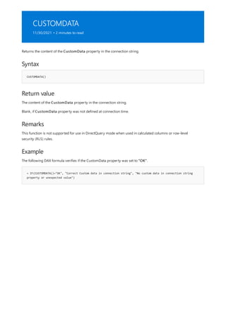
![HASONEFILTER
11/30/2021 • 2 minutes to read
Syntax
HASONEFILTER(<columnName>)
Parameters
TERM DEFINITION
columnName The name of an existing column, using standard DAX syntax.
It cannot be an expression.
Return value
Remarks
Example
= IF(HASONEFILTER(ResellerSales_USD[ProductKey]),FILTERS(ResellerSales_USD[ProductKey]),BLANK())
Returns TRUE when the number of directly filtered values on columnName is one; otherwise returns FALSE.
TRUE when the number of directly filtered values on columnName is one; otherwise returns FALSE.
This function is similar to HASONEVALUE() with the difference that HASONEVALUE() works based on
cross-filters while HASONEFILTER() works by a direct filter.
This function is not supported for use in DirectQuery mode when used in calculated columns or row-
level security (RLS) rules.
The following example shows how to use HASONEFILTER() to return the filter for
ResellerSales_USD[ProductKey]) if there is one filter, or to return BLANK if there are no filters or more than one
filter on ResellerSales_USD[ProductKey]).](https://image.slidesharecdn.com/funcoesdax-220812141017-bb6cd4dc/85/Funcoes-DAX-pdf-305-320.jpg)
![HASONEVALUE
11/30/2021 • 2 minutes to read
Syntax
HASONEVALUE(<columnName>)
Parameters
TERM DEFINITION
columnName The name of an existing column, using standard DAX syntax.
It cannot be an expression.
Return value
Remarks
Example
=
IF(HASONEVALUE(DateTime[CalendarYear]),SUM(ResellerSales_USD[SalesAmount_USD])/CALCULATE(SUM(ResellerSales_U
SD[SalesAmount_USD]),DateTime[CalendarYear]=2007),BLANK())
Returns TRUE when the context for columnName has been filtered down to one distinct value only. Otherwise is
FALSE.
TRUE when the context for columnName has been filtered down to one distinct value only. Otherwise is FALSE.
An equivalent expression for HASONEVALUE() is COUNTROWS(VALUES(<columnName>)) = 1 .
This function is not supported for use in DirectQuery mode when used in calculated columns or row-
level security (RLS) rules.
The following measure formula verifies if the context is being sliced by one value in order to estimate a
percentage against a predefined scenario; in this case you want to compare Reseller Sales against sales in 2007,
then you need to know if the context is filtered by single years. Also, if the comparison is meaningless you want
to return BLANK.](https://image.slidesharecdn.com/funcoesdax-220812141017-bb6cd4dc/85/Funcoes-DAX-pdf-306-320.jpg)
![ISAFTER
11/30/2021 • 2 minutes to read
Syntax
ISAFTER(<scalar_expression>, <scalar_expression>[, sort_order [, <scalar_expression>, <scalar_expression>[,
sort_order]]…)
Parameters
TERM DEFINITION
scalar expression Any expression that returns a scalar value like a column
reference or integer or string value. Typically the first
parameter is a column reference and the second parameter
is a scalar value.
sort order (optional) The order in which the column is sorted. Can be
ascending (ASC) or descending (DEC). By default the sort
order is ascending.
Return value
Remarks
Example
COUNTRY STATE COUNT TOTAL
IND JK 20 800
IND MH 25 1000
A boolean function that emulates the behavior of a 'Start At' clause and returns true for a row that meets all of
the condition parameters.
Based on the sort order, the first parameter is compared with the second parameter. If the sort order is
ascending, the comparison to be done is first parameter greater than the second parameter. If the sort order is
descending, the comparison to be done is second parameter less than the first parameter.
True or false.
This function is similar to ISONORAFTER. The difference is ISAFTER returns true for values sorted strictly after
the filter values, where ISONORAFTER returns true for values sorted on or after the filter values.
This function is not supported for use in DirectQuery mode when used in calculated columns or row-level
security (RLS) rules.
Table name: 'Info'](https://image.slidesharecdn.com/funcoesdax-220812141017-bb6cd4dc/85/Funcoes-DAX-pdf-307-320.jpg)
![IND WB 10 900
USA CA 5 500
USA WA 10 900
COUNTRY STATE COUNT TOTAL
FILTER (
Info,
ISAFTER (
Info[Country], "IND", ASC,
Info[State], "MH", ASC )
)
COUNTRY STATE COUNT TOTAL
IND WB 10 900
USA CA 5 500
USA WA 10 900
See also
The following expression:
Returns:
ISONORAFTER](https://image.slidesharecdn.com/funcoesdax-220812141017-bb6cd4dc/85/Funcoes-DAX-pdf-308-320.jpg)
![ISBLANK
11/30/2021 • 2 minutes to read
Syntax
ISBLANK(<value>)
Parameters
TERM DEFINITION
value The value or expression you want to test.
Return value
Remarks
Example
//Sales to Previous Year Ratio
= IF( ISBLANK('CalculatedMeasures'[PreviousYearTotalSales])
, BLANK()
, ( 'CalculatedMeasures'[Total Sales]-'CalculatedMeasures'[PreviousYearTotalSales] )
/'CalculatedMeasures'[PreviousYearTotalSales])
ROW LABELS TOTAL SALES
TOTAL SALES PREVIOUS
YEAR
SALES TO PREVIOUS YEAR
RATIO
2005 $10,209,985.08
2006 $28,553,348.43 $10,209,985.08 179.66%
2007 $39,248,847.52 $28,553,348.43 37.46%
2008 $24,542,444.68 $39,248,847.52 -37.47%
Grand Total $102,554,625.71
Checks whether a value is blank, and returns TRUE or FALSE.
A Boolean value of TRUE if the value is blank; otherwise FALSE.
To learn more about best practices when working with BLANKS, see Avoid converting BLANKs to values in DAX.
This formula computes the increase or decrease ratio in sales compared to the previous year. The example uses
the IF function to check the value for the previous year's sales in order to avoid a divide by zero error.
Result,](https://image.slidesharecdn.com/funcoesdax-220812141017-bb6cd4dc/85/Funcoes-DAX-pdf-309-320.jpg)

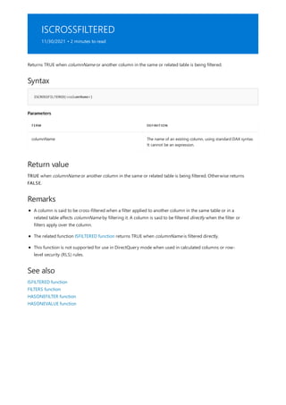
![ISEMPTY
11/30/2021 • 2 minutes to read
Syntax
ISEMPTY(<table_expression>)
Parameters
TERM DEFINITION
table_expression A table reference or a DAX expression that returns a table.
Return value
Remarks
Example
COUNTRY STATE COUNTY TOTAL
IND JK 20 800
IND MH 25 1000
IND WB 10 900
USA CA 5 500
USA WA 10 900
EVALUATE
ROW("Any countries with count > 25?", NOT(ISEMPTY(FILTER(Info, [County]>25))))
Checks if a table is empty.
True if the table is empty (has no rows), if else, False.
This function is not supported for use in DirectQuery mode when used in calculated columns or row-level
security (RLS) rules.
For the below table named 'Info':
Return value: FALSE](https://image.slidesharecdn.com/funcoesdax-220812141017-bb6cd4dc/85/Funcoes-DAX-pdf-312-320.jpg)
![ISERROR
11/30/2021 • 2 minutes to read
Syntax
ISERROR(<value>)
Parameters
TERM DEFINITION
value The value you want to test.
Return value
Remarks
Example
= IF( ISERROR(
SUM('ResellerSales_USD'[SalesAmount_USD])
/SUM('InternetSales_USD'[SalesAmount_USD])
)
, BLANK()
, SUM('ResellerSales_USD'[SalesAmount_USD])
/SUM('InternetSales_USD'[SalesAmount_USD])
)
See also
Checks whether a value is an error, and returns TRUE or FALSE.
A Boolean value of TRUE if the value is an error; otherwise FALSE.
For best practices when using ISERROR, see Appropriate use of error functions.
This function is not supported for use in DirectQuery mode when used in calculated columns or row-
level security (RLS) rules.
The following example calculates the ratio of total Internet sales to total reseller sales. The ISERROR function is
used to check for errors, such as division by zero. If there is an error a blank is returned, otherwise the ratio is
returned.
Information functions
IFERROR function
IF function](https://image.slidesharecdn.com/funcoesdax-220812141017-bb6cd4dc/85/Funcoes-DAX-pdf-313-320.jpg)

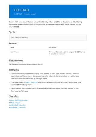
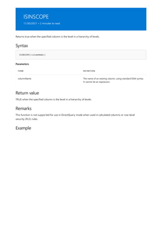
![DEFINE
MEASURE FactInternetSales[% of Parent] =
SWITCH (TRUE(),
ISINSCOPE(DimProduct[Subcategory]),
DIVIDE(
SUM(FactInternetSales[Sales Amount]),
CALCULATE(
SUM(FactInternetSales[Sales Amount]),
ALLSELECTED(DimProduct[Subcategory]))
),
ISINSCOPE(DimProduct[Category]),
DIVIDE(
SUM(FactInternetSales[Sales Amount]),
CALCULATE(
SUM(FactInternetSales[Sales Amount]),
ALLSELECTED(DimProduct[Category]))
),
1
) * 100
EVALUATE
SUMMARIZECOLUMNS
(
ROLLUPADDISSUBTOTAL
(
DimProduct[Category], "Category Subtotal",
DimProduct[Subcategory], "Subcategory Subtotal"
),
TREATAS(
{"Bike Racks", "Bike Stands", "Mountain Bikes", "Road Bikes", "Touring Bikes"},
DimProduct[Subcategory]),
"Sales", SUM(FactInternetSales[Sales Amount]),
"% of Parent", [% of Parent]
)
ORDER BY
[Category Subtotal] DESC, [Category],
[Subcategory Subtotal] DESC, [Subcategory]
DIMPRODUCT[C
ATEGORY]
DIMPRODUCT[S
UBCATEGORY]
[CATEGORY
SUBTOTAL]
[SUBCATEGORY
SUBTOTAL] [SALES] [% OF PARENT]
TRUE TRUE 28,397,095.65 100.00
Accessories FALSE TRUE 78,951.00 0.28
Accessories Bike Racks FALSE FALSE 39,360.00 49.85
Accessories Bike Stands FALSE FALSE 39,591.00 50.15
Bikes FALSE TRUE 28,318,144.65 99.72
Bikes Mountain Bikes FALSE FALSE 9,952,759.56 35.15
Bikes Road Bikes FALSE FALSE 14,520,584.04 51.28
Bikes Touring Bikes FALSE FALSE 3,844,801.05 13.58
See also
Returns,](https://image.slidesharecdn.com/funcoesdax-220812141017-bb6cd4dc/85/Funcoes-DAX-pdf-317-320.jpg)

![ISONORAFTER
11/30/2021 • 2 minutes to read
Syntax
ISONORAFTER(<scalar_expression>, <scalar_expression>[, sort_order [, <scalar_expression>,
<scalar_expression>[, sort_order]]…)
Parameters
TERM DEFINITION
scalar expression Any expression that returns a scalar value like a column
reference or integer or string value. Typically the first
parameter is a column reference and the second parameter
is a scalar value.
sort order (optional) The order in which the column is sorted. Can be
ascending (ASC) or descending (DEC). By default the sort
order is ascending.
Return value
Remarks
Example
COUNTRY STATE COUNT TOTAL
IND JK 20 800
IND MH 25 1000
A boolean function that emulates the behavior of a Start At clause and returns true for a row that meets all of
the condition parameters.
Based on the sort order, the first parameter is compared with the second parameter. If the sort order is
ascending, the comparison to be done is first parameter greater than the second parameter. If the sort order is
descending, the comparison to be done is second parameter less than the first parameter.
True or false.
This function is similar to ISAFTER. The difference is ISONORAFTER returns true for values sorted on or after the
filter values, where ISAFTER returns true for values sorted strictly after the filter values.
This function is not supported for use in DirectQuery mode when used in calculated columns or row-level
security (RLS) rules.
Table name: 'Info'](https://image.slidesharecdn.com/funcoesdax-220812141017-bb6cd4dc/85/Funcoes-DAX-pdf-323-320.jpg)
![IND WB 10 900
USA CA 5 500
USA WA 10 900
COUNTRY STATE COUNT TOTAL
FILTER (
Info,
ISONORAFTER (
Info[Country], "IND", ASC,
Info[State], "MH", ASC )
)
COUNTRY STATE COUNT TOTAL
IND MH 25 1000
IND WB 10 900
USA CA 5 500
USA WA 10 900
See also
The following expression:
Returns:
ISAFTER](https://image.slidesharecdn.com/funcoesdax-220812141017-bb6cd4dc/85/Funcoes-DAX-pdf-324-320.jpg)
![ISSELECTEDMEASURE
11/30/2021 • 2 minutes to read
Syntax
ISSELECTEDMEASURE( M1, M2, ... )
Parameters
TERM DEFINITION
M1, M2, ... A list of measures.
Return value
Remarks
Example
IF (
ISSELECTEDMEASURE ( [Expense Ratio 1], [Expense Ratio 2] ),
SELECTEDMEASURE (),
DIVIDE ( SELECTEDMEASURE (), COUNTROWS ( DimDate ) )
)
See also
Used by expressions for calculation items to determine the measure that is in context is one of those specified in
a list of measures.
A Boolean indicating whether the measure that is currently in context is one of those specified in the list of
parameters.
Can only be referenced in the expression for a calculation item.
This function is not supported for use in DirectQuery mode when used in calculated columns or row-
level security (RLS) rules.
The following calculation item expression checks if the current measure is one of those specified in the list of
parameters. If the measures are renamed, formula fixup will reflect the name changes in the expression.
SELECTEDMEASURE
SELECTEDMEASURENAME](https://image.slidesharecdn.com/funcoesdax-220812141017-bb6cd4dc/85/Funcoes-DAX-pdf-325-320.jpg)
![ISSUBTOTAL
11/30/2021 • 2 minutes to read
Syntax
ISSUBTOTAL(<columnName>)
SUMMARIZE(<table>, <groupBy_columnName>[, <groupBy_columnName>]…[, ROLLUP(<groupBy_columnName>[,<
groupBy_columnName>…])][, <name>, {<expression>|ISSUBTOTAL(<columnName>)}]…)
Parameters
TERM DEFINITION
columnName The name of any column in table of the SUMMARIZE
function or any column in a related table to table.
Return value
Remarks
Example
Creates another column in a SUMMARIZE expression that returns True if the row contains subtotal values for the
column given as argument, otherwise returns False.
With SUMMARIZE,
A True value if the row contains a subtotal value for the column given as argument, otherwise returns False.
This function can only be used in the expression of a SUMMARIZE function.
This function must be preceded by the name of the Boolean column.
See SUMMARIZE.](https://image.slidesharecdn.com/funcoesdax-220812141017-bb6cd4dc/85/Funcoes-DAX-pdf-326-320.jpg)
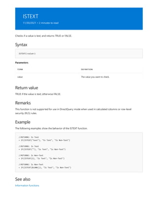
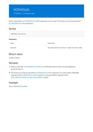
![SELECTEDMEASURE
11/30/2021 • 2 minutes to read
Syntax
SELECTEDMEASURE()
Parameters
Return value
Remarks
Example
CALCULATE(SELECTEDMEASURE(), DATESYTD(DimDate[Date]))
See also
Used by expressions for calculation items to reference the measure that is in context.
None
A reference to the measure that is currently in context when the calculation item is evaluated.
Can only be referenced in the expression for a calculation item.
This function is not supported for use in DirectQuery mode when used in calculated columns or row-
level security (RLS) rules.
The following calculation item expression calculates the year-to-date for whatever the measure is in context.
SELECTEDMEASURENAME
ISSELECTEDMEASURE](https://image.slidesharecdn.com/funcoesdax-220812141017-bb6cd4dc/85/Funcoes-DAX-pdf-329-320.jpg)
![SELECTEDMEASUREFORMATSTRING
11/30/2021 • 2 minutes to read
Syntax
SELECTEDMEASUREFORMATSTRING()
Parameters
Return value
Remarks
Example
SELECTEDVALUE( DimCurrency[FormatString], SELECTEDMEASUREFORMATSTRING() )
See also
Used by expressions for calculation items to retrieve the format string of the measure that is in context.
None
A string holding the format string of the measure that is currently in context when the calculation item is
evaluated.
This function can only be referenced in expressions for calculation items in calculation groups. It is
designed to be used by the Format String Expression property of calculation items.
This function is not supported for use in DirectQuery mode when used in calculated columns or row-
level security (RLS) rules.
The following expression is evaluated by the Format String Expression property for a calculation item. If there is
a single currency in filter context, the format string is retrieved from the DimCurrency[FormatString] column;
otherwise the format string of the measure in context is used.
SELECTEDMEASURE
ISSELECTEDMEASURE](https://image.slidesharecdn.com/funcoesdax-220812141017-bb6cd4dc/85/Funcoes-DAX-pdf-330-320.jpg)
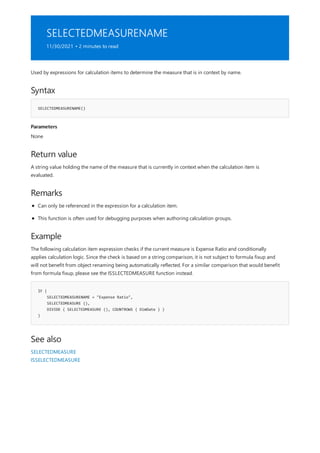
![USERNAME
11/30/2021 • 2 minutes to read
Syntax
USERNAME()
Parameters
Return value
Example
= IF(CONTAINS(UsersTable,UsersTable[login], USERNAME()), "Allowed", BLANK())
Returns the domain name and username from the credentials given to the system at connection time.
This expression has no parameters.
The username from the credentials given to the system at connection time
The following formula verifies if the user login is part of the UsersTable.](https://image.slidesharecdn.com/funcoesdax-220812141017-bb6cd4dc/85/Funcoes-DAX-pdf-332-320.jpg)
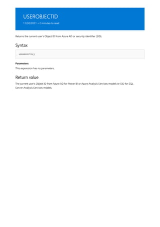
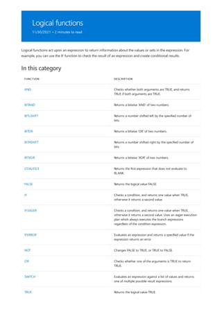
![AND
11/30/2021 • 2 minutes to read
Syntax
AND(<logical1>,<logical2>)
Parameters
TERM DEFINITION
logical_1, logical_2 The logical values you want to test.
Return value
Remarks
Example 1
= IF(AND(10 > 9, -10 < -1), "All true", "One or more false"
Example 2
= IF( AND( SUM( 'InternetSales_USD'[SalesAmount_USD])
>SUM('ResellerSales_USD'[SalesAmount_USD])
, CALCULATE(SUM('InternetSales_USD'[SalesAmount_USD]), PREVIOUSYEAR('DateTime'[DateKey] ))
>CALCULATE(SUM('ResellerSales_USD'[SalesAmount_USD]), PREVIOUSYEAR('DateTime'[DateKey] ))
)
, "Internet Hit"
, ""
)
Checks whether both arguments are TRUE, and returns TRUE if both arguments are TRUE. Otherwise returns
false.
Returns true or false depending on the combination of values that you test.
The AND function in DAX accepts only two (2) arguments. If you need to perform an AND operation on multiple
expressions, you can create a series of calculations or, better, use the AND operator (&&) to join all of them in a
simpler expression.
The following formula shows the syntax of the AND function.
Because both conditions, passed as arguments, to the AND function are true, the formula returns "All True".
The following sample uses the AND function with nested formulas to compare two sets of calculations at the
same time. For each product category, the formula determines if the current year sales and previous year sales
of the Internet channel are larger than the Reseller channel for the same periods. If both conditions are true, for
each category the formula returns the value, "Internet hit".](https://image.slidesharecdn.com/funcoesdax-220812141017-bb6cd4dc/85/Funcoes-DAX-pdf-336-320.jpg)
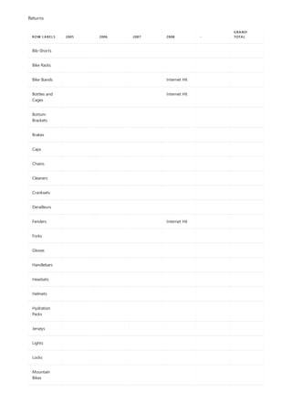
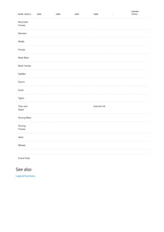
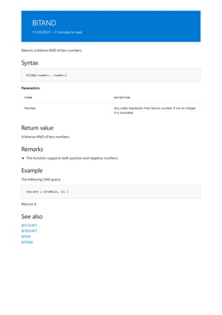
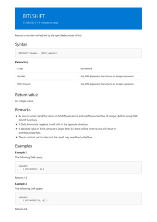
![Example 3
Define
Measure Sales[LeftShift] = BITLSHIFT(SELECTEDVALUE(Sales[Amount]), 3)
EVALUATE
SUMMARIZECOLUMNS(
Sales[Amount],
"LEFTSHIFT",
[LeftShift]
)
See also
The following DAX query:
Shifts left each sales amount with 3 bits and returns the bit-shifted sales amount.
BITRSHIFT
BITAND
BITOR
BITXOR](https://image.slidesharecdn.com/funcoesdax-220812141017-bb6cd4dc/85/Funcoes-DAX-pdf-341-320.jpg)
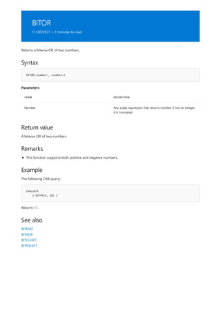

![Example 3
Define
Measure Sales[RightShift] = BITRSHIFT(SELECTEDVALUE(Sales[Amount]), 3)
EVALUATE
SUMMARIZECOLUMNS(
Sales[Amount],
"RIGHTSHIFT",
[RightShift]
)
See also
The following DAX query:
Shifts right each sales amount with 3 bits and returns the bit-shifted sales amount.
BITLSHIFT
BITAND
BITOR
BITXOR](https://image.slidesharecdn.com/funcoesdax-220812141017-bb6cd4dc/85/Funcoes-DAX-pdf-344-320.jpg)

![COALESCE
11/30/2021 • 2 minutes to read
Syntax
COALESCE(<expression>, <expression>[, <expression>]…)
Parameters
TERM DEFINITION
expression Any DAX expression that returns a scalar expression.
Return value
Remarks
Example 1
EVALUATE { COALESCE(BLANK(), 10, DATE(2008, 3, 3)) }
Example 2
= COALESCE(SUM(FactInternetSales[SalesAmount]), 0)
Returns the first expression that does not evaluate to BLANK. If all expressions evaluate to BLANK, BLANK is
returned.
A scalar value coming from one of the expressions or BLANK if all expressions evaluate to BLANK.
Input expressions may be of different data types.
The following DAX query:
Returns 10 , which is the first expression that does not evaluate to BLANK.
The following DAX expression:
Returns the sum of all values in the SalesAmount column in the FactInternetSales table, or 0 . This can be used
to convert BLANK values of total sales to 0 .](https://image.slidesharecdn.com/funcoesdax-220812141017-bb6cd4dc/85/Funcoes-DAX-pdf-346-320.jpg)
![FALSE
11/30/2021 • 2 minutes to read
Syntax
FALSE()
Return value
Remarks
Example
= IF(SUM('InternetSales_USD'[SalesAmount_USD]) >200000, TRUE(), false())
ROW LABELS 2005 2006 2007 2008 -
GRAND
TOTAL
Accessories FALSE FALSE TRUE TRUE FALSE TRUE
Bikes TRUE TRUE TRUE TRUE FALSE TRUE
Clothing FALSE FALSE FALSE FALSE FALSE TRUE
Components FALSE FALSE FALSE FALSE FALSE FALSE
FALSE FALSE FALSE FALSE FALSE FALSE
Grand Total TRUE TRUE TRUE TRUE FALSE TRUE
See also
Returns the logical value FALSE.
Always FALSE.
The word FALSE is also interpreted as the logical value FALSE.
The formula returns the logical value FALSE when the value in the column,
'InternetSales_USD'[SalesAmount_USD], is less than or equal to 200000.
The following table shows the results when the example formula is used with
'ProductCategory'[ProductCategoryName] in Row Labels and 'DateTime'[CalendarYear] in Column Labels.
TRUE function
NOT function
IF function](https://image.slidesharecdn.com/funcoesdax-220812141017-bb6cd4dc/85/Funcoes-DAX-pdf-347-320.jpg)
![IF
11/30/2021 • 2 minutes to read
Syntax
IF(<logical_test>, <value_if_true>[, <value_if_false>])
Parameters
TERM DEFINITION
logical_test Any value or expression that can be evaluated to TRUE or
FALSE.
value_if_true The value that's returned if the logical test is TRUE.
value_if_false (Optional) The value that's returned if the logical test is
FALSE. If omitted, BLANK is returned.
Return value
Remarks
Examples
Checks a condition, and returns one value when it's TRUE, otherwise it returns a second value.
Either value_if_true, value_if_false, or BLANK.
The IF function can return a variant data type if value_if_true and value_if_false are of different data
types, but the function attempts to return a single data type if both value_if_true and value_if_false
are of numeric data types. In the latter case, the IF function will implicitly convert data types to
accommodate both values.
For example, the formula IF(<condition>, TRUE(), 0) returns TRUE or 0, but the formula
IF(<condition>, 1.0, 0) returns only decimal values even though value_if_false is of the whole
number data type. To learn more about implicit data type conversion, see Data types.
To execute the branch expressions regardless of the condition expression, use IF.EAGER instead.
The following Product table calculated column definitions use the IF function in different ways to classify each
product based on its list price.
The first example tests whether the List Price column value is less than 500. When this condition is true, the
value Low is returned. Because there's no value_if_false value, BLANK is returned.
Examples in this article can be added to the Power BI Desktop sample model. To get the model, see DAX sample
model.](https://image.slidesharecdn.com/funcoesdax-220812141017-bb6cd4dc/85/Funcoes-DAX-pdf-348-320.jpg)
![Price Group =
IF(
'Product'[List Price] < 500,
"Low"
)
Price Group =
IF(
'Product'[List Price] < 500,
"Low",
"High"
)
Price Group =
IF(
'Product'[List Price] < 500,
"Low",
IF(
'Product'[List Price] < 1500,
"Medium",
"High"
)
)
TIP
See also
The second example uses the same test, but this time includes a value_if_false value. So, the formula classifies
each product as either Low or High.
The third example uses the same test, but this time nests an IF function to perform an additional test. So, the
formula classifies each product as either Low, Medium, or High.
When you need to nest multiple IF functions, the SWITCH function might be a better option. This function provides a
more elegant way to write an expression that returns more than two possible values.
IF.EAGER function
SWITCH function (DAX)
Logical functions](https://image.slidesharecdn.com/funcoesdax-220812141017-bb6cd4dc/85/Funcoes-DAX-pdf-349-320.jpg)
![IF.EAGER
11/30/2021 • 2 minutes to read
Syntax
IF.EAGER(<logical_test>, <value_if_true>[, <value_if_false>])
Parameters
TERM DEFINITION
logical_test Any value or expression that can be evaluated to TRUE or
FALSE.
value_if_true The value that's returned if the logical test is TRUE.
value_if_false (Optional) The value that's returned if the logical test is
FALSE. If omitted, BLANK is returned.
Return value
Remarks
Checks a condition, and returns one value when TRUE, otherwise it returns a second value. It uses an eager
execution plan which always executes the branch expressions regardless of the condition expression.
Either value_if_true, value_if_false, or BLANK.
VAR _value_if_true = <value_if_true>
VAR _value_if_false = <value_if_false>
RETURN
IF (<logical_test>, _value_if_true, _value_if_false)
The IF.EAGER function can return a variant data type if value_if_true and value_if_false are of different
data types, but the function attempts to return a single data type if both value_if_true and
value_if_false are of numeric data types. In the latter case, the IF.EAGER function will implicitly convert
data types to accommodate both values.
For example, the formula IF.EAGER(<condition>, TRUE(), 0) returns TRUE or 0, but the formula
IF.EAGER(<condition>, 1.0, 0) returns only decimal values even though value_if_false is of the whole
number data type. To learn more about implicit data type conversion, see Data types.
IF.EAGER has the same functional behavior as the IF function, but performance may differ due to
differences in execution plans. IF.EAGER(<logical_test>, <value_if_true>, <value_if_false>) has the
same execution plan as the following DAX expression:
Note: The two branch expressions are evaluated regardless of the condition expression.](https://image.slidesharecdn.com/funcoesdax-220812141017-bb6cd4dc/85/Funcoes-DAX-pdf-350-320.jpg)
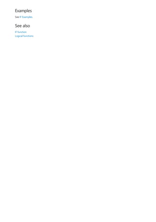
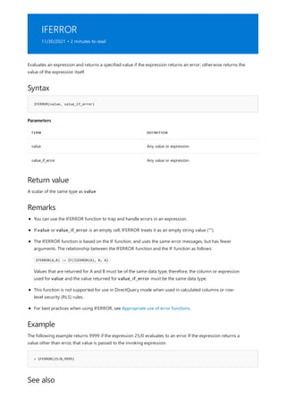

![NOT
11/30/2021 • 2 minutes to read
Syntax
NOT(<logical>)
Parameters
TERM DEFINITION
logical A value or expression that can be evaluated to TRUE or
FALSE.
Return value
Example
= NOT([CalculatedColumn1])
See also
Changes FALSE to TRUE, or TRUE to FALSE.
TRUE OR FALSE.
The following example retrieves values from the calculated column that was created to illustrate the IF function.
For that example, the calculated column was named using the default name, Calculated Column1, and
contains the following formula: = IF([Orders]<300,"true","false")
The formula checks the value in the column, [Orders], and returns "true" if the number of orders is under 300.
Now create a new calculated column, Calculated Column2, and type the following formula.
For each row in Calculated Column1, the values "true" and "false" are interpreted as the logical values TRUE or
FALSE, and the NOT function returns the logical opposite of that value.
TRUE function
FALSE function
IF function](https://image.slidesharecdn.com/funcoesdax-220812141017-bb6cd4dc/85/Funcoes-DAX-pdf-354-320.jpg)
![OR
11/30/2021 • 2 minutes to read
Syntax
OR(<logical1>,<logical2>)
Parameters
TERM DEFINITION
logical_1, logical_2 The logical values you want to test.
Return value
Remarks
Example
IF( OR( CALCULATE(SUM('ResellerSales_USD'[SalesAmount_USD]),
'ProductSubcategory'[ProductSubcategoryName]="Touring Bikes") > 1000000
, CALCULATE(SUM('ResellerSales_USD'[SalesAmount_USD]), 'DateTime'[CalendarYear]=2007) > 2500000
)
, "Circle of Excellence"
, ""
)
ROW LABELS 2005 2006 2007 2008 -
GRAND
TOTAL
Abbas, Syed E
Checks whether one of the arguments is TRUE to return TRUE. The function returns FALSE if both arguments are
FALSE.
A Boolean value. The value is TRUE if any of the two arguments is TRUE; the value is FALSE if both the
arguments are FALSE.
The OR function in DAX accepts only two (2) arguments. If you need to perform an OR operation on
multiple expressions, you can create a series of calculations or, better, use the OR operator (||) to join all of
them in a simpler expression.
The function evaluates the arguments until the first TRUE argument, then returns TRUE.
The following example shows how to use the OR function to obtain the sales people that belong to the Circle of
Excellence. The Circle of Excellence recognizes those who have achieved more than a million dollars in Touring
Bikes sales or sales of over two and a half million dollars in 2007.
Returns](https://image.slidesharecdn.com/funcoesdax-220812141017-bb6cd4dc/85/Funcoes-DAX-pdf-355-320.jpg)
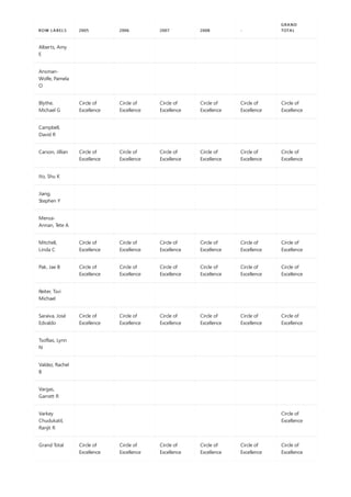

![SWITCH
11/30/2021 • 2 minutes to read
Syntax
SWITCH(<expression>, <value>, <result>[, <value>, <result>]…[, <else>])
Parameters
TERM DEFINITION
expression Any DAX expression that returns a single scalar value, where
the expression is to be evaluated multiple times (for each
row/context).
value A constant value to be matched with the results of
expression.
result Any scalar expression to be evaluated if the results of
expression match the corresponding value.
else Any scalar expression to be evaluated if the result of
expression doesn't match any of the value arguments.
Return value
Remarks
Example
= SWITCH([Month], 1, "January", 2, "February", 3, "March", 4, "April"
, 5, "May", 6, "June", 7, "July", 8, "August"
, 9, "September", 10, "October", 11, "November", 12, "December"
, "Unknown month number" )
Evaluates an expression against a list of values and returns one of multiple possible result expressions.
A scalar value coming from one of the result expressions, if there was a match with value, or from the else
expression, if there was no match with any value.
All result expressions and the else expression must be of the same data type.
The following example creates a calculated column of month names.](https://image.slidesharecdn.com/funcoesdax-220812141017-bb6cd4dc/85/Funcoes-DAX-pdf-358-320.jpg)
![TRUE
11/30/2021 • 2 minutes to read
Syntax
TRUE()
Return value
Remarks
Example
= IF(SUM('InternetSales_USD'[SalesAmount_USD]) >200000, TRUE(), false())
ROW LABELS 2005 2006 2007 2008 -
GRAND
TOTAL
Accessories FALSE FALSE TRUE TRUE FALSE TRUE
Bikes TRUE TRUE TRUE TRUE FALSE TRUE
Clothing FALSE FALSE FALSE FALSE FALSE TRUE
Components FALSE FALSE FALSE FALSE FALSE FALSE
FALSE FALSE FALSE FALSE FALSE FALSE
Grand Total TRUE TRUE TRUE TRUE FALSE TRUE
See also
Returns the logical value TRUE.
Always TRUE.
The word TRUE is also interpreted as the logical value TRUE.
The formula returns the logical value TRUE when the value in the column,
'InternetSales_USD'[SalesAmount_USD], is greater than 200000.
The following table shows the results when the example formula is used in a report with
'ProductCategory'[ProductCategoryName] in Row Labels and 'DateTime'[CalendarYear] in Column Labels.
FALSE
NOT
IF](https://image.slidesharecdn.com/funcoesdax-220812141017-bb6cd4dc/85/Funcoes-DAX-pdf-359-320.jpg)
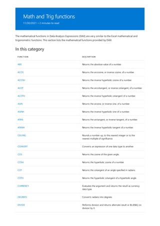
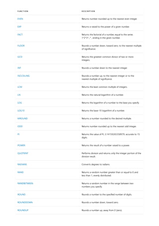
![ABS
11/30/2021 • 2 minutes to read
Syntax
ABS(<number>)
Parameters
TERM DEFINITION
number The number for which you want the absolute value.
Return value
Remarks
Example
= ABS([DealerPrice]-[ListPrice])
See also
Returns the absolute value of a number.
A decimal number.
The absolute value of a number is a decimal number, whole or decimal, without its sign. You can use the ABS
function to ensure that only non-negative numbers are returned from expressions when nested in functions that
require a positive number.
The following example returns the absolute value of the difference between the list price and the dealer price,
which you might use in a new calculated column, DealerMarkup.
Math and Trig functions
SIGN function](https://image.slidesharecdn.com/funcoesdax-220812141017-bb6cd4dc/85/Funcoes-DAX-pdf-363-320.jpg)

![Example 2
= CEILING([ProductPrice],0.05)
See also
The following formula returns similar results as the previous example, but uses numeric values stored in the
column, ProductPrice.
Math and Trig functions
FLOOR function
ISO.CEILING function
ROUNDUP function](https://image.slidesharecdn.com/funcoesdax-220812141017-bb6cd4dc/85/Funcoes-DAX-pdf-373-320.jpg)
![CONVERT
11/30/2021 • 2 minutes to read
Syntax
CONVERT(<Expression>, <Datatype>)
Parameters
TERM DEFINITION
Expression Any valid expression.
Datatype An enumeration that includes: INTEGER(Whole Number),
DOUBLE(Decimal Number), STRING(Text),
BOOLEAN(True/False), CURRENCY(Fixed Decimal Number),
DATETIME(Date, Time, etc).
Return value
Remarks
Example
EVALUATE { CONVERT(DATE(1900, 1, 1), INTEGER) }
[VALUE]
2
Converts an expression of one data type to another.
Returns the value of <Expression>, translated to <Datatype>.
The function returns an error when a value cannot be converted to the specified data type.
DAX calculated columns must be of a single data type. Since MEDIAN and MEDIANX functions over an
integer column return mixed data types, either integer or double, the following calculated column
expression will return an error as a result: MedianNumberCarsOwned = MEDIAN(DimCustomer[NumberCarsOwned]) .
To avoid mixed data types, change the expression to always return the double data type, for example:
MedianNumberCarsOwned = MEDIANX(DimCustomer, CONVERT([NumberCarsOwned], DOUBLE)) .
This function is not supported for use in DirectQuery mode when used in calculated columns or row-
level security (RLS) rules.
DAX query
Returns](https://image.slidesharecdn.com/funcoesdax-220812141017-bb6cd4dc/85/Funcoes-DAX-pdf-374-320.jpg)
![COT
11/30/2021 • 2 minutes to read
Syntax
COT (<number>)
Parameters
TERM DEFINITION
number The angle in radians for which you want the cotangent.
Return value
Remarks
Example
EVALUATE { COT(30) }
[VALUE]
-0.156119952161659
Returns the cotangent of an angle specified in radians.
The cotangent of the given angle.
The absolute value of number must be less than 2^27 and cannot be 0.
If number is outside its constraints, an error is returned.
If number is a non-numeric value, an error is returned.
The following DAX query,
Returns](https://image.slidesharecdn.com/funcoesdax-220812141017-bb6cd4dc/85/Funcoes-DAX-pdf-377-320.jpg)
![COTH
11/30/2021 • 2 minutes to read
Syntax
COTH (<number>)
Parameters
TERM DEFINITION
number The hyperbolic angle in radians for which you want the
hyperbolic cotangent.
Return value
Remarks
Example
EVALUATE { COTH(2) }
[VALUE]
1.03731472072755
Returns the hyperbolic cotangent of a hyperbolic angle.
The hyperbolic cotangent of the given angle.
The hyperbolic cotangent is an analog of the ordinary (circular) cotangent.
The absolute value of number must be less than $2^{27}$ and cannot be 0.
If number is outside its constraints, an error is returned
If number is a non-numeric value, an error is returned.
The following equation is used:
$$text{COTH}(N) = frac{1}{text{TANH}(N)} = frac{text{COSH(N)}}{text{SINH(N)}} = frac{e^{N} + e^{-
N}}{e^{N} - e^{-N}}$$
This function is not supported for use in DirectQuery mode when used in calculated columns or row-
level security (RLS) rules.
The following DAX query,
Returns](https://image.slidesharecdn.com/funcoesdax-220812141017-bb6cd4dc/85/Funcoes-DAX-pdf-378-320.jpg)
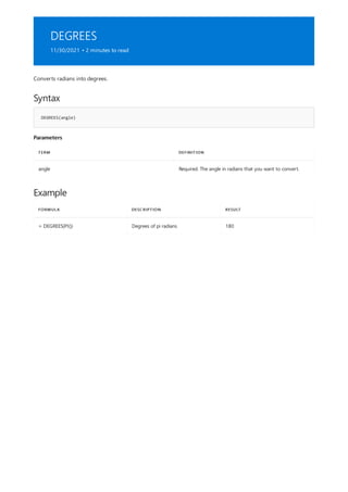
![DIVIDE
11/30/2021 • 2 minutes to read
Syntax
DIVIDE(<numerator>, <denominator> [,<alternateresult>])
Parameters
TERM DEFINITION
numerator The dividend or number to divide.
denominator The divisor or number to divide by.
alternateresult (Optional) The value returned when division by zero results
in an error. When not provided, the default value is BLANK().
Return value
Remarks
Example
= DIVIDE(5,2)
Example 1
= DIVIDE(5,0)
Example 2
Performs division and returns alternate result or BLANK() on division by 0.
A decimal number.
Alternate result on divide by 0 must be a constant.
For best practices when using DIVIDE, see DIVIDE function vs. divide operator (/) in DAX.
The following example returns 2.5.
The following example returns BLANK.
The following example returns 1.](https://image.slidesharecdn.com/funcoesdax-220812141017-bb6cd4dc/85/Funcoes-DAX-pdf-381-320.jpg)
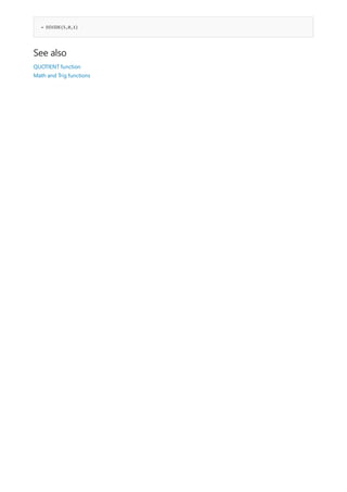
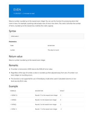
![EXP
11/30/2021 • 2 minutes to read
Syntax
EXP(<number>)
Parameters
TERM DEFINITION
number The exponent applied to the base e. The constant e equals
2.71828182845904, the base of the natural logarithm.
Return value
Exceptions
Remarks
Example
= EXP([Power])
See also
Returns e raised to the power of a given number. The constant e equals 2.71828182845904, the base of the
natural logarithm.
A decimal number.
EXP is the inverse of LN, which is the natural logarithm of the given number.
To calculate powers of bases other than e, use the exponentiation operator (^). For more information, see
DAX Operator Reference.
The following formula calculates e raised to the power of the number contained in the column, [Power] .
Math and Trig functions
LN function
EXP function
LOG function
LOG function](https://image.slidesharecdn.com/funcoesdax-220812141017-bb6cd4dc/85/Funcoes-DAX-pdf-384-320.jpg)
![FACT
11/30/2021 • 2 minutes to read
Syntax
FACT(<number>)
Parameters
TERM DEFINITION
number The non-negative number for which you want to calculate
the factorial.
Return value
Remarks
Example
= FACT([Values])
VALUES RESULTS
0 1
1 1
2 2
3 6
4 24
Returns the factorial of a number, equal to the series 1*2*3*...* , ending in the given number.
A decimal number.
If the number is not an integer, it is truncated and an error is returned. If the result is too large, an error is
returned.
This function is not supported for use in DirectQuery mode when used in calculated columns or row-
level security (RLS) rules.
The following formula returns the factorial for the series of integers in the column, [Values] .
The following table shows the expected results:](https://image.slidesharecdn.com/funcoesdax-220812141017-bb6cd4dc/85/Funcoes-DAX-pdf-385-320.jpg)
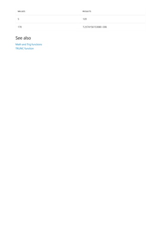
![FLOOR
11/30/2021 • 2 minutes to read
Syntax
FLOOR(<number>, <significance>)
Parameters
TERM DEFINITION
number The numeric value you want to round.
significance The multiple to which you want to round. The
argumentsnumber and significance must either both be
positive, or both be negative.
Return value
Remarks
Example
= FLOOR(InternetSales[Total Product Cost],.5)
VALUES EXPECTED RESULT
10.8423 10.8
8.0373 8
Rounds a number down, toward zero, to the nearest multiple of significance.
A decimal number.
If either argument is nonnumeric, FLOOR returns **#VALUE!**error value.
If number and significance have different signs, FLOOR returns the **#NUM!**error value.
Regardless of the sign of the number, a value is rounded down when adjusted away from zero. If the
number is an exact multiple of significance, no rounding occurs.
This function is not supported for use in DirectQuery mode when used in calculated columns or row-
level security (RLS) rules.
The following formula takes the values in the [Total Product Cost] column from the table, InternetSales.and
rounds down to the nearest multiple of .1.
The following table shows the expected results for some sample values.](https://image.slidesharecdn.com/funcoesdax-220812141017-bb6cd4dc/85/Funcoes-DAX-pdf-387-320.jpg)
![GCD
11/30/2021 • 2 minutes to read
Syntax
GCD(number1, [number2], ...)
Parameters
TERM DEFINITION
number1, number2, ... Number1 is required, subsequent numbers are optional. 1 to
255 values. If any value is not an integer, it is truncated.
Return value
Remarks
Example
FORMULA DESCRIPTION RESULT
= GCD(5, 2) Greatest common divisor of 5 and 2. 1
= GCD(24, 36) Greatest common divisor of 24 and
36.
12
= GCD(7, 1) Greatest common divisor of 7 and 1. 1
Returns the greatest common divisor of two or more integers. The greatest common divisor is the largest
integer that divides both number1 and number2 without a remainder.
The greatest common divisor of two or more integers.
If any argument is nonnumeric, GCD returns the #VALUE! error value.
If any argument is less than zero, GCD returns the #NUM! error value.
One divides any value evenly.
A prime number has only itself and one as even divisors.
If a parameter to GCD is >=2^53, GCD returns the #NUM! error value.
This function is not supported for use in DirectQuery mode when used in calculated columns or row-
level security (RLS) rules.](https://image.slidesharecdn.com/funcoesdax-220812141017-bb6cd4dc/85/Funcoes-DAX-pdf-389-320.jpg)
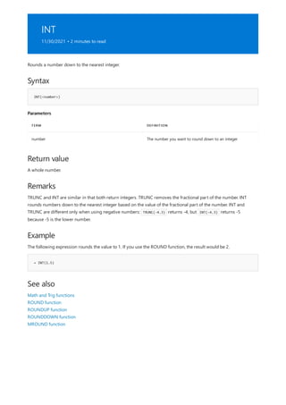
![ISO.CEILING
11/30/2021 • 2 minutes to read
Syntax
ISO.CEILING(<number>[, <significance>])
Parameters
TERM DEFINITION
number The number you want to round, or a reference to a column
that contains numbers.
significance (optional) The multiple of significance to which you want to
round. For example, to round to the nearest integer, type 1.
If the unit of significance is not specified, the number is
rounded up to the nearest integer.
Return value
Remarks
Example: Positive Numbers
Rounds a number up, to the nearest integer or to the nearest multiple of significance.
A number, of the same type as the number argument, rounded as specified.
There are two CEILING functions in DAX, with the following differences:
The CEILING function emulates the behavior of the CEILING function in Excel.
The ISO.CEILING function follows the ISO-defined behavior for determining the ceiling value.
The two functions return the same value for positive numbers, but different values for negative numbers. When
using a positive multiple of significance, both CEILING and ISO.CEILING round negative numbers upward
(toward positive infinity). When using a negative multiple of significance, CEILING rounds negative numbers
downward (toward negative infinity), while ISO.CEILING rounds negative numbers upward (toward positive
infinity).
The result type is usually the same type of the significance used as argument with the following exceptions:
If the first argument is of currency type then the result will be currency type.
If the optional argument is not included the result is of integer type.
If the significance argument is of Boolean type then the result is of integer type.
If the significance argument is non-numeric type then the result is of real type.
The following formula returns 4.45. This might be useful if you want to avoid using smaller units in your pricing.](https://image.slidesharecdn.com/funcoesdax-220812141017-bb6cd4dc/85/Funcoes-DAX-pdf-391-320.jpg)
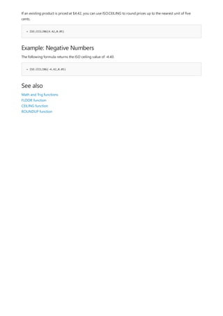
![LCM
11/30/2021 • 2 minutes to read
Syntax
LCM(number1, [number2], ...)
Parameters
TERM DEFINITION
number1, number2,... Number1 is required, subsequent numbers are optional. 1 to
255 values for which you want the least common multiple. If
value is not an integer, it is truncated.
Return value
Remarks
Example
FORMULA DESCRIPTION RESULT
= LCM(5, 2) Least common multiple of 5 and 2. 10
= LCM(24, 36) Least common multiple of 24 and 36. 72
Returns the least common multiple of integers. The least common multiple is the smallest positive integer that is
a multiple of all integer arguments number1, number2, and so on. Use LCM to add fractions with different
denominators.
Returns the least common multiple of integers.
If any argument is nonnumeric, LCM returns the #VALUE! error value.
If any argument is less than zero, LCM returns the #NUM! error value.
If LCM(a,b) >=2^53, LCM returns the #NUM! error value.
This function is not supported for use in DirectQuery mode when used in calculated columns or row-
level security (RLS) rules.](https://image.slidesharecdn.com/funcoesdax-220812141017-bb6cd4dc/85/Funcoes-DAX-pdf-393-320.jpg)
![LN
11/30/2021 • 2 minutes to read
Syntax
LN(<number>)
Parameters
TERM DEFINITION
number The positive number for which you want the natural
logarithm.
Return value
Remarks
Example
= LN([Values])
See also
Returns the natural logarithm of a number. Natural logarithms are based on the constant e
(2.71828182845904).
A decimal number.
LN is the inverse of the EXP function.
The following example returns the natural logarithm of the number in the column, [Values] .
Math and Trig functions
EXP function](https://image.slidesharecdn.com/funcoesdax-220812141017-bb6cd4dc/85/Funcoes-DAX-pdf-394-320.jpg)
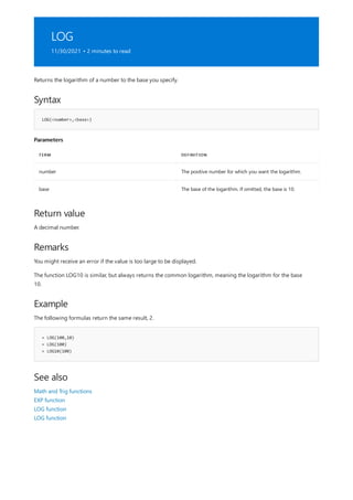


![PI
11/30/2021 • 2 minutes to read
Syntax
PI()
Return value
Remarks
Example
= PI()*([Radius]*2)
See also
Returns the value of Pi, 3.14159265358979, accurate to 15 digits.
A decimal number with the value of Pi, 3.14159265358979, accurate to 15 digits.
Pi is a mathematical constant. In DAX, Pi is represented as a real number accurate to 15 digits, the same as Excel.
The following formula calculates the area of a circle given the radius in the column, [Radius] .
Math and Trig functions](https://image.slidesharecdn.com/funcoesdax-220812141017-bb6cd4dc/85/Funcoes-DAX-pdf-402-320.jpg)

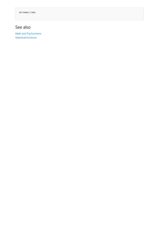
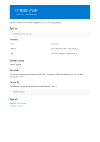
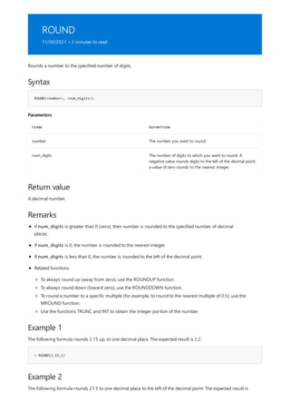
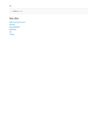
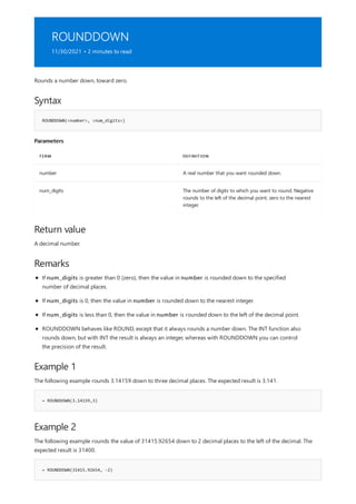

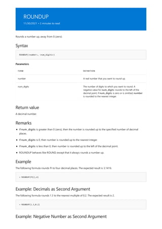
![= ROUNDUP([Values],-1)
FREIGHTCOST EXPECTED RESULT
13.25 20
2.45 10
25.56 30
1.34 10
345.01 350
See also
The following formula rounds the value in the column, FreightCost, with the expected results shown in the
following table:
When num_digits is less than zero, the number of places to the left of the decimal sign is increased by the
value you specify.
Math and Trig functions
ROUND
ROUNDDOWN
MROUND
INT](https://image.slidesharecdn.com/funcoesdax-220812141017-bb6cd4dc/85/Funcoes-DAX-pdf-414-320.jpg)
![SIGN
11/30/2021 • 2 minutes to read
Syntax
SIGN(<number>)
Parameters
TERM DEFINITION
number Any real number, a column that contains numbers, or an
expression that evaluates to a number.
Return value
RETURN VALUE DESCRIPTION
1 The number is positive
0 The number is zero
-1 The number is negative
Example
= SIGN( ([Sale Price] - [Cost]) )
See also
Determines the sign of a number, the result of a calculation, or a value in a column. The function returns 1 if the
number is positive, 0 (zero) if the number is zero, or -1 if the number is negative.
A whole number. The possible Return values are 1, 0, and -1.
The following formula returns the sign of the result of the expression that calculates sale price minus cost.
Math and Trig functions](https://image.slidesharecdn.com/funcoesdax-220812141017-bb6cd4dc/85/Funcoes-DAX-pdf-415-320.jpg)
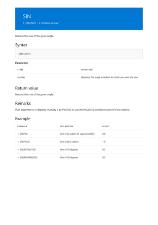
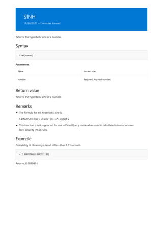
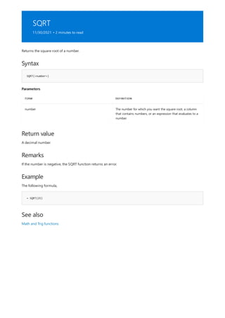

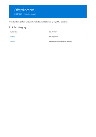
![BLANK
11/30/2021 • 2 minutes to read
Syntax
BLANK()
Return value
Remarks
Example
= IF( SUM(InternetSales_USD[SalesAmount_USD])= 0 , BLANK() ,
SUM(ResellerSales_USD[SalesAmount_USD])/SUM(InternetSales_USD[SalesAmount_USD]) )
ROW LABELS ACCESSORIES BIKES CLOTHING GRAND TOTAL
2005 2.65 2.89
2006 3.33 4.03
2007 1.04 2.92 6.63 3.51
2008 0.41 1.53 2.00 1.71
Grand Total 0.83 2.51 5.45 2.94
Returns a blank.
A blank.
Blanks are not equivalent to nulls. DAX uses blanks for both database nulls and for blank cells in Excel.
Some DAX functions treat blank cells somewhat differently from Microsoft Excel. Blanks and empty
strings ("") are not always equivalent, but some operations may treat them as such.
The following example illustrates how you can work with blanks in formulas. The formula calculates the ratio of
sales between the Resellers and the Internet channels. However, before attempting to calculate the ratio the
denominator should be checked for zero values. If the denominator is zero then a blank value should be
returned; otherwise, the ratio is calculated.
The table shows the expected results when this formula is used to create a table visualization.
In the original data source, the column evaluated by the BLANK function might have included text, empty
strings, or nulls. If the original data source was a SQL Server database, nulls and empty strings are different
kinds of data. However, for this operation an implicit type cast is performed and DAX treats them as the same.](https://image.slidesharecdn.com/funcoesdax-220812141017-bb6cd4dc/85/Funcoes-DAX-pdf-425-320.jpg)

![ERROR
11/30/2021 • 2 minutes to read
Syntax
ERROR(<text>)
Parameters
TERM DEFINITION
text A text string containing an error message.
Return value
Remarks
Example 1
DEFINE
MEASURE DimProduct[Measure] =
IF(
SELECTEDVALUE(DimProduct[Color]) = "Red",
ERROR("red color encountered"),
SELECTEDVALUE(DimProduct[Color])
)
EVALUATE SUMMARIZECOLUMNS(DimProduct[Color], "Measure", [Measure])
ORDER BY [Color]
Example 2
Raises an error with an error message.
None
The ERROR function can be placed in a DAX expression anywhere a scalar value is expected.
This function is not supported for use in DirectQuery mode when used in calculated columns or row-
level security (RLS) rules.
The following DAX query:
Fails and raises and error message containing "red color encountered".
The following DAX query:](https://image.slidesharecdn.com/funcoesdax-220812141017-bb6cd4dc/85/Funcoes-DAX-pdf-427-320.jpg)
![DEFINE
MEASURE DimProduct[Measure] =
IF(
SELECTEDVALUE(DimProduct[Color]) = "Magenta",
ERROR("magenta color encountered"),
SELECTEDVALUE(DimProduct[Color])
)
EVALUATE SUMMARIZECOLUMNS(DimProduct[Color], "Measure", [Measure])
ORDER BY [Color]
DIMPRODUCT[COLOR] [MEASURE]
Black Black
Blue Blue
Grey Grey
Multi Multi
NA NA
Red Red
Silver Silver
SilverBlack SilverBlack
White White
Yellow Yellow
Returns the following table:
Because Magenta is not one of the product colors, the ERROR function is not executed.](https://image.slidesharecdn.com/funcoesdax-220812141017-bb6cd4dc/85/Funcoes-DAX-pdf-428-320.jpg)
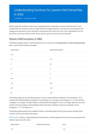
![14 112 112|14
3 14 112|14|3
11 3 112|14|3|11
13 3 112|14|3|13
162 3 112|14|3|162
117 162 112|14|3|162|117
221 162 112|14|3|162|221
81 162 112|14|3|162|81
EMPLOYEEKEY PARENTEMPLOYEEKEY PATH
EMPLOYEEKEY PARENTEMPLOYEEKEY PATH PATHLENGTH
112 112 1
14 112 112|14 2
3 14 112|14|3 3
11 3 112|14|3|11 4
13 3 112|14|3|13 4
162 3 112|14|3|162 4
117 162 112|14|3|162|117 5
221 162 112|14|3|162|221 5
81 162 112|14|3|162|81 5
EMPLOYEEKEY PARENTEMPLOYEEKEY PATH
PATHITEM - 4TH FROM
LEFT
112 112
14 112 112|14
PATHLENGTH function - Returns the number of levels in a given PATH(), starting at current level until the oldest
or top most parent level. In the following example column PathLength is defined as ' = PATHLENGTH([Path]) '; the
example includes all data from the Path() example to help understand how this function works.
PATHITEM function - Returns the item at the specified position from a PATH() like result, counting from left to
right. In the following example column PathItem - 4th from left is defined as ' = PATHITEM([Path], 4) '; this
example returns the EmployeKey at fourth position in the Path string from the left, using the same sample data
from the Path() example.](https://image.slidesharecdn.com/funcoesdax-220812141017-bb6cd4dc/85/Funcoes-DAX-pdf-431-320.jpg)
![3 14 112|14|3
11 3 112|14|3|11 11
13 3 112|14|3|13 13
162 3 112|14|3|162 162
117 162 112|14|3|162|117 162
221 162 112|14|3|162|221 162
81 162 112|14|3|162|81 162
EMPLOYEEKEY PARENTEMPLOYEEKEY PATH
PATHITEM - 4TH FROM
LEFT
EMPLOYEEKEY PARENTEMPLOYEEKEY PATH
PATHITEMREVERSE - 3RD
FROM RIGHT
112 112
14 112 112|14
3 14 112|14|3 112
11 3 112|14|3|11 14
13 3 112|14|3|13 14
162 3 112|14|3|162 14
117 162 112|14|3|162|117 3
221 162 112|14|3|162|221 3
81 162 112|14|3|162|81 3
PATHITEMREVERSE function - Returns the item at position from a PATH() like function result, counting backwards
from right to left.
In the following example column PathItemReverse - 3rd from right is defined as ' = PATHITEMREVERSE([Path], 3) ';
this example returns the EmployeKey at third position in the Path string from the right, using the same sample
data from the Path() example.
PATHCONTAINS function - Returns TRUE if the specified item exists within the specified path. In the following
example column PathContains - employee 162 is defined as ' = PATHCONTAINS([Path], "162") '; this example
returns TRUE if the given path contains employee 162. This example uses the results from the Path() example
above.](https://image.slidesharecdn.com/funcoesdax-220812141017-bb6cd4dc/85/Funcoes-DAX-pdf-432-320.jpg)
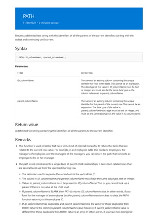
![Example
= PATH(Employee[EmployeeKey], Employee[ParentEmployeeKey])
the same employee ID and they have the same manager ID, the PATH function returns the ID for that
manager. However, if there are two identical employee IDs that have different manager IDs, the PATH
function returns an error.
If ID_columnName is BLANK then PATH() returns BLANK.
If ID_columnName contains a vertical bar '|' then PATH() returns an error.
This function is not supported for use in DirectQuery mode when used in calculated columns or row-
level security (RLS) rules.
The following example creates a calculated column that lists all the managers for each employee.](https://image.slidesharecdn.com/funcoesdax-220812141017-bb6cd4dc/85/Funcoes-DAX-pdf-435-320.jpg)
![PATHCONTAINS
11/30/2021 • 2 minutes to read
Syntax
PATHCONTAINS(<path>, <item>)
Parameters
TERM DEFINITION
path A string created as the result of evaluating a PATH function.
item A text expression to look for in the path result.
Return value
Remarks
Example
= PATHCONTAINS(PATH(Employee[EmployeeKey], Employee[ParentEmployeeKey]), "23")
Returns TRUE if the specified item exists within the specified path.
A value of TRUE if item exists in path; otherwise FALSE.
If item is an integer number it is converted to text and then the function is evaluated. If conversion fails
then the function returns an error.
This function is not supported for use in DirectQuery mode when used in calculated columns or row-
level security (RLS) rules.
The following example creates a calculated column that takes a manager ID and checks a set of employees. If the
manager ID is among the list of managers returned by the PATH function, the PATHCONTAINS function returns
true; otherwise it returns false.](https://image.slidesharecdn.com/funcoesdax-220812141017-bb6cd4dc/85/Funcoes-DAX-pdf-436-320.jpg)
![PATHITEM
11/30/2021 • 2 minutes to read
Syntax
PATHITEM(<path>, <position>[, <type>])
Parameters
TERM DEFINITION
path A text string in the form of the results of a PATH function.
position An integer expression with the position of the item to be
returned.
type (Optional)An enumeration that defines the data type of the
result:
type enumeration
ENUMERATION ALTERNATE ENUMERATION DESCRIPTION
TEXT 0 Results are returned with the data type
text. (default).
INTEGER 1 Results are returned as integers.
Return value
Remarks
Example
Returns the item at the specified position from a string resulting from evaluation of a PATH function. Positions
are counted from left to right.
The identifier returned by the PATH function at the specified position in the list of identifiers. Items returned by
the PATH function are ordered by most distant to current.
This function can be used to return a specific level from a hierarchy returned by a PATH function. For
example, you could return just the skip-level managers for all employees.
If you specify a number for position that is less than one (1) or greater than the number of elements in
path, the PATHITEM function returns BLANK
If type is not a valid enumeration element an error is returned.
This function is not supported for use in DirectQuery mode when used in calculated columns or row-
level security (RLS) rules.](https://image.slidesharecdn.com/funcoesdax-220812141017-bb6cd4dc/85/Funcoes-DAX-pdf-437-320.jpg)
![= PATHITEM(PATH(Employee[EmployeeKey], Employee[ParentEmployeeKey]), 3, 1)
The following example returns the third tier manager of the current employee; it takes the employee and
manager IDs as the input to a PATH function that returns a string with the hierarchy of parents to current
employee. From that string PATHITEM returns the third entry as an integer.](https://image.slidesharecdn.com/funcoesdax-220812141017-bb6cd4dc/85/Funcoes-DAX-pdf-438-320.jpg)
![PATHITEMREVERSE
11/30/2021 • 2 minutes to read
Syntax
PATHITEMREVERSE(<path>, <position>[, <type>])
Parameters
TERM DEFINITION
path A text string resulting from evaluation of a PATH function.
position An integer expression with the position of the item to be
returned. Position is counted backwards from right to left.
type (Optional)An enumeration that defines the data type of the
result:
type enumeration
ENUMERATION ALTERNATE ENUMERATION DESCRIPTION
TEXT 0 Results are returned with the data type
text. (default).
INTEGER 1 Results are returned as integers.
Return value
Remarks
Returns the item at the specified position from a string resulting from evaluation of a PATH function. Positions
are counted backwards from right to left.
The n-position ascendant in the given path, counting from current to the oldest.
This function can be used to get an individual item from a hierarchy resulting from a PATH function.
This function reverses the standard order of the hierarchy, so that closest items are listed first, For
example, if the PATh function returns a list of managers above an employee in a hierarchy, the
PATHITEMREVERSE function returns the employee's immediate manager in position 2 because position 1
contains the employee's id.
If the number specified for position is less than one (1) or greater than the number of elements in path,
the PATHITEM function returns BLANK.
If type is not a valid enumeration element an error is returned.
This function is not supported for use in DirectQuery mode when used in calculated columns or row-
level security (RLS) rules.](https://image.slidesharecdn.com/funcoesdax-220812141017-bb6cd4dc/85/Funcoes-DAX-pdf-439-320.jpg)
![Example
= PATHITEMREVERSE(PATH(Employee[EmployeeKey], Employee[ParentEmployeeKey]), 3, 1)
The following example takes an employee ID column as the input to a PATH function, and reverses the list of
grandparent elements that are returned. The position specified is 3 and the return type is 1; therefore, the
PATHITEMREVERSE function returns an integer representing the manager two levels up from the employee.](https://image.slidesharecdn.com/funcoesdax-220812141017-bb6cd4dc/85/Funcoes-DAX-pdf-440-320.jpg)
![PATHLENGTH
11/30/2021 • 2 minutes to read
Syntax
PATHLENGTH(<path>)
Parameters
TERM DEFINITION
path A text expression resulting from evaluation of a PATH
function.
Return value
Remarks
Example
= PATHLENGTH(PATH(Employee[EmployeeKey], Employee[ParentEmployeeKey]))
Returns the number of parents to the specified item in a given PATH result, including self.
The number of items that are parents to the specified item in a given PATH result, including the specified item.
This function is not supported for use in DirectQuery mode when used in calculated columns or row-level
security (RLS) rules.
The following example takes an employee ID as input to a PATH function and returns a list of the managers
above that employee in the hierarchy, The PATHLENGTH function takes that result and counts the different levels
of employees and managers, including the employee you started with.](https://image.slidesharecdn.com/funcoesdax-220812141017-bb6cd4dc/85/Funcoes-DAX-pdf-441-320.jpg)
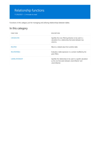
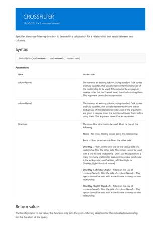
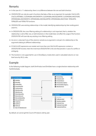
![BiDi:= CALCULATE([Distinct Count of ProductKey], CROSSFILTER(FactInternetSales[ProductKey],
DimProduct[ProductKey] , Both))
There are two ways to get the count of products by year:
Turn on bi-directional cross-filtering on the relationship. This will change how filters work for all data
between these two tables.
Use the CROSSFILTER function to change how the relationships work for just this measure.
When using DAX, we can use the CROSSFILTER function to change how the cross-filter direction behaves
between two columns defined by a relationship. In this case, the DAX expression looks like this:
By using the CROSSFILTER function in our measure expression, we get the expected results:](https://image.slidesharecdn.com/funcoesdax-220812141017-bb6cd4dc/85/Funcoes-DAX-pdf-445-320.jpg)
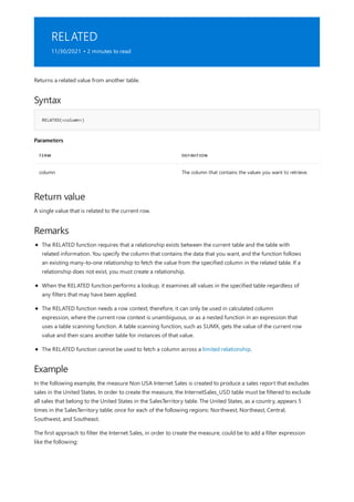
![FILTER('InternetSales_USD'
, 'InternetSales_USD'[SalesTerritoryKey]<>1 && 'InternetSales_USD'[SalesTerritoryKey]<>2 &&
'InternetSales_USD'[SalesTerritoryKey]<>3 && 'InternetSales_USD'[SalesTerritoryKey]<>4 &&
'InternetSales_USD'[SalesTerritoryKey]<>5)
FILTER( 'InternetSales_USD', RELATED('SalesTerritory'[SalesTerritoryCountry])<>"United States")
NOTE
= SUMX(FILTER( 'InternetSales_USD'
, RELATED('SalesTerritory'[SalesTerritoryCountry])
<>"United States"
)
,'InternetSales_USD'[SalesAmount_USD])
ROW LABELS INTERNET SALES NON USA INTERNET SALES
Australia $4,999,021.84 $4,999,021.84
Canada $1,343,109.10 $1,343,109.10
France $2,490,944.57 $2,490,944.57
Germany $2,775,195.60 $2,775,195.60
United Kingdom $5,057,076.55 $5,057,076.55
United States $9,389,479.79
Grand Total $26,054,827.45 $16,665,347.67
ROW LABELS ACCESSORIES BIKES CLOTHING GRAND TOTAL
2005 $1,526,481.95 $1,526,481.95
However, this approach is counterintuitive, prone to typing errors, and might not work if any of the existing
regions is split in the future.
A better approach would be to use the existing relationship between InternetSales_USD and SalesTerritory and
explicitly state that the country must be different from the United States. To do so, create a filter expression like
the following:
This expression uses the RELATED function to lookup the country value in the SalesTerritory table, starting with
the value of the key column, SalesTerritoryKey, in the InternetSales_USD table. The result of the lookup is used
by the filter function to determine if the InternetSales_USD row is filtered or not.
If the example does not work, you might need to create a relationship between the tables.
The following table shows only totals for each region, to prove that the filter expression in the measure, Non
USA Internet Sales, works as intended.
The following shows what that you might get if you used this measure in a report table visual:](https://image.slidesharecdn.com/funcoesdax-220812141017-bb6cd4dc/85/Funcoes-DAX-pdf-447-320.jpg)
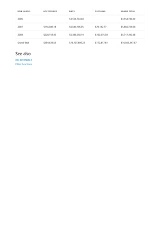
![RELATEDTABLE
11/30/2021 • 2 minutes to read
Syntax
RELATEDTABLE(<tableName>)
Parameters
TERM DEFINITION
tableName The name of an existing table using standard DAX syntax. It
cannot be an expression.
Return value
Remarks
Example
= SUMX( RELATEDTABLE('InternetSales_USD')
, [SalesAmount_USD])
PRODUCT CATEGORY KEY
PRODUCT CATEGORY
ALTERNATEKEY
PRODUCT CATEGORY
NAME INTERNET SALES
1 1 Bikes $28,318,144.65
2 2 Components
3 3 Clothing $339,772.61
Evaluates a table expression in a context modified by the given filters.
A table of values.
The RELATEDTETABLE function changes the context in which the data is filtered, and evaluates the
expression in the new context that you specify.
This function is a shortcut for CALCULATETABLE function with no logical expression.
This function is not supported for use in DirectQuery mode when used in calculated columns or row-
level security (RLS) rules.
The following example uses the RELATEDTABLE function to create a calculated column with the Internet Sales in
the Product Category table:
The following table shows the results:](https://image.slidesharecdn.com/funcoesdax-220812141017-bb6cd4dc/85/Funcoes-DAX-pdf-449-320.jpg)
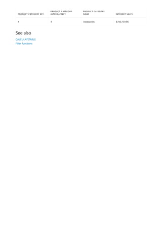
![USERELATIONSHIP
11/30/2021 • 2 minutes to read
Syntax
USERELATIONSHIP(<columnName1>,<columnName2>)
Parameters
TERM DEFINITION
columnName1 The name of an existing column, using standard DAX syntax
and fully qualified, that usually represents the many side of
the relationship to be used; if the arguments are given in
reverse order the function will swap them before using them.
This argument cannot be an expression.
columnName2 The name of an existing column, using standard DAX syntax
and fully qualified, that usually represents the one side or
lookup side of the relationship to be used; if the arguments
are given in reverse order the function will swap them before
using them. This argument cannot be an expression.
Return value
Remarks
Specifies the relationship to be used in a specific calculation as the one that exists between columnName1 and
columnName2.
The function returns no value; the function only enables the indicated relationship for the duration of the
calculation.
USERELATIONSHIP can only be used in functions that take a filter as an argument, for example:
CALCULATE, CALCULATETABLE, CLOSINGBALANCEMONTH, CLOSINGBALANCEQUARTER,
CLOSINGBALANCEYEAR, OPENINGBALANCEMONTH, OPENINGBALANCEQUARTER,
OPENINGBALANCEYEAR, TOTALMTD, TOTALQTD and TOTALYTD functions.
USERELATIONSHIP cannot be used when row level security is defined for the table in which the measure
is included. For example,
CALCULATE(SUM([SalesAmount]), USERELATIONSHIP(FactInternetSales[CustomerKey],
DimCustomer[CustomerKey]))
will return an error if row level security is defined for DimCustomer.
USERELATIONSHIP uses existing relationships in the model, identifying relationships by their ending
point columns.
In USERELATIONSHIP, the status of a relationship is not important; that is, whether the relationship is
active or not does not affect the usage of the function. Even if the relationship is inactive, it will be used
and overrides any other active relationships that might be present in the model but not mentioned in the
function arguments.](https://image.slidesharecdn.com/funcoesdax-220812141017-bb6cd4dc/85/Funcoes-DAX-pdf-451-320.jpg)
![Example
= CALCULATE(SUM(InternetSales[SalesAmount]), USERELATIONSHIP(InternetSales[ShippingDate], DateTime[Date]))
An error is returned if any of the columns named as an argument is not part of a relationship or the
arguments belong to different relationships.
If multiple relationships are needed to join table A to table B in a calculation, each relationship must be
indicated in a different USERELATIONSHIP function.
If CALCULATE expressions are nested, and more than one CALCULATE expression contains a
USERELATIONSHIP function, then the innermost USERELATIONSHIP is the one that prevails in case of a
conflict or ambiguity.
Up to 10 USERELATIONSHIP functions can be nested; however, your expression might have a deeper level
of nesting, ie. the following sample expression is nested 3 levels deep but only 2 for USEREALTIONSHIP:
=CALCULATE(CALCULATE( CALCULATE( <anyExpression>, USERELATIONSHIP( t1[colA], t2[colB])),
t99[colZ]=999), USERELATIONSHIP( t1[colA], t2[colA]))
.
For 1-to-1 relationships, USERELATIONSHIP will only activate the relationship in one direction. In
particular, filters will only be able to flow from columnName2's table to columnName1's table. If bi-
directional cross-filtering is desired, two USERELATIONSHIPs with opposite directionality can be used in
the same calculation. For example,
CALCULATE(..., USERELATIONSHIP(T1[K], T2[K]), USERELATIONSHIP(T2[K], T1[K])) .
The following sample shows how to override the default, active, relationship between InternetSales and
DateTime tables. The default relationship exists between the OrderDate column, in the InternetSales table, and
the Date column, in the DateTime table.
To calculate the sum of internet sales and allow slicing by ShippingDate instead of the traditional OrderDate,
create measure, [InternetSales by ShippingDate] using the following expression:
Relationships between InternetSales[ShipmentDate] and DateTime[Date] must exist and should not be the active
relationship; also, the relationship between InternetSales[OrderDate] and DateTime[Date] should exist and
should be the active relationship.](https://image.slidesharecdn.com/funcoesdax-220812141017-bb6cd4dc/85/Funcoes-DAX-pdf-452-320.jpg)

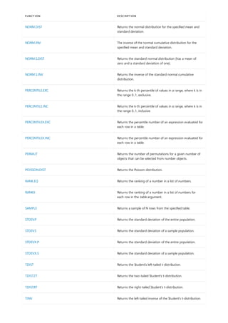
![BETA.DIST
11/30/2021 • 2 minutes to read
Syntax
BETA.DIST(x,alpha,beta,cumulative,[A],[B])
Parameters
TERM DEFINITION
x The value between A and B at which to evaluate the function
Alpha A parameter of the distribution.
Beta A parameter of the distribution.
A Optional. A lower bound to the interval of x.
B Optional. An upper bound to the interval of x.
Return value
Remarks
Returns the beta distribution. The beta distribution is commonly used to study variation in the percentage of
something across samples, such as the fraction of the day people spend watching television.
Returns the beta distribution.
If any argument is nonnumeric, BETA.DIST returns the #VALUE! error value.
If any argument is not an integer, it is rounded.
If alpha ≤ 0 or beta ≤ 0, BETA.DIST returns the #NUM! error value.
If x < A, x > B, or A = B, BETA.DIST returns the #NUM! error value.
If you omit values for A and B, BETA.DIST uses the standard cumulative beta distribution, so that A = 0
and B = 1.
This function is not supported for use in DirectQuery mode when used in calculated columns or row-
level security (RLS) rules.](https://image.slidesharecdn.com/funcoesdax-220812141017-bb6cd4dc/85/Funcoes-DAX-pdf-456-320.jpg)
![BETA.INV
11/30/2021 • 2 minutes to read
Syntax
BETA.INV(probability,alpha,beta,[A],[B])
Parameters
TERM DEFINITION
Probability A probability associated with the beta distribution.
Alpha A parameter of the distribution.
Beta A parameter the distribution.
A Optional. A lower bound to the interval of x.
B Optional. An upper bound to the interval of x.
Return value
Remarks
Returns the inverse of the beta cumulative probability density function (BETA.DIST).
If probability = BETA.DIST(x,...TRUE), then BETA.INV(probability,...) = x. The beta distribution can be used in project
planning to model probable completion times given an expected completion time and variability.
Returns the inverse of the beta cumulative probability density function (BETA.DIST).
If any argument is nonnumeric, BETA.INV returns the #VALUE! error value.
If any argument is not an integer, it is rounded.
If alpha ≤ 0 or beta ≤ 0, BETA.INV returns the #NUM! error value.
If probability ≤ 0 or probability > 1, BETA.INV returns the #NUM! error value.
If you omit values for A and B, BETA.INV uses the standard cumulative beta distribution, so that A = 0 and
B = 1.
This function is not supported for use in DirectQuery mode when used in calculated columns or row-
level security (RLS) rules.](https://image.slidesharecdn.com/funcoesdax-220812141017-bb6cd4dc/85/Funcoes-DAX-pdf-457-320.jpg)
![[VALUE]
0.632120558828558](https://image.slidesharecdn.com/funcoesdax-220812141017-bb6cd4dc/85/Funcoes-DAX-pdf-459-320.jpg)
![CHISQ.DIST.RT
11/30/2021 • 2 minutes to read
Syntax
CHISQ.DIST.RT(<x>, <deg_freedom>)
Parameters
TERM DEFINITION
x The value at which you want to evaluate the distribution.
Deg_freedom The number of degrees of freedom.
Return value
Remarks
Example
EVALUATE { CHISQ.DIST.RT(2, 5) }
[VALUE]
0.84914503608461
Returns the right-tailed probability of the chi-squared distribution.
The chi-squared distribution is associated with a chi-squared test. Use the chi-squared test to compare observed
and expected values. For example, a genetic experiment might hypothesize that the next generation of plants will
exhibit a certain set of colors. By comparing the observed results with the expected ones, you can decide
whether your original hypothesis is valid.
The right-tailed probability of the chi-squared distribution.
If x or deg_freedom is nonnumeric, an error is returned.
If deg_freedom is not an integer, it is rounded.
If x < 0, an error is returned.
If deg_freedom < 1 or deg_freedom > 10^10, an error is returned.
This function is not supported for use in DirectQuery mode when used in calculated columns or row-
level security (RLS) rules.
The following DAX query,
Returns](https://image.slidesharecdn.com/funcoesdax-220812141017-bb6cd4dc/85/Funcoes-DAX-pdf-460-320.jpg)
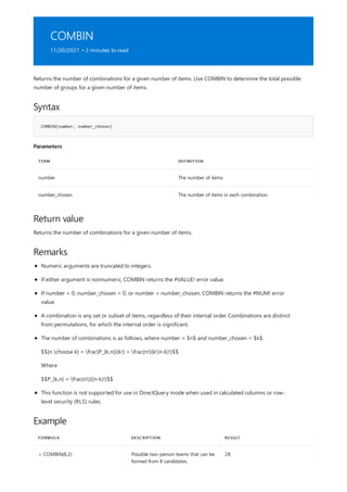
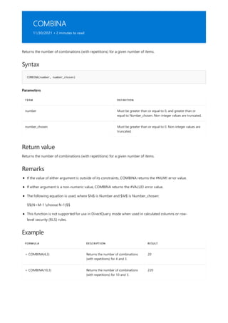
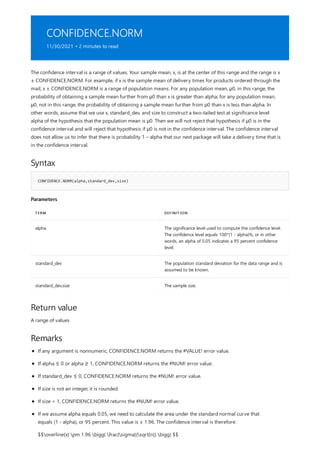
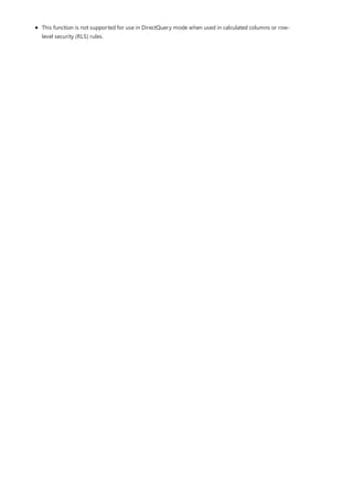
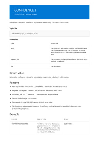
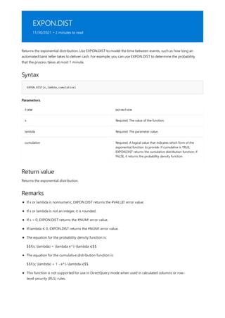
![GEOMEAN
11/30/2021 • 2 minutes to read
Syntax
GEOMEAN(<column>)
Parameters
TERM DEFINITION
column The column that contains the numbers for which the
geometric mean is to be computed.
Return value
Remarks
Example
= GEOMEAN( Investment[Return] )
See also
Returns the geometric mean of the numbers in a column.
To return the geometric mean of an expression evaluated for each row in a table, use GEOMEANX function.
A decimal number.
Only the numbers in the column are counted. Blanks, logical values, and text are ignored.
GEOMEAN( Table[Column] ) is equivalent to GEOMEANX( Table, Table[Column] )
This function is not supported for use in DirectQuery mode when used in calculated columns or row-
level security (RLS) rules.
The following computes the geometric mean of the Return column in the Investment table:
GEOMEANX function](https://image.slidesharecdn.com/funcoesdax-220812141017-bb6cd4dc/85/Funcoes-DAX-pdf-469-320.jpg)
![GEOMEANX
11/30/2021 • 2 minutes to read
Syntax
GEOMEANX(<table>, <expression>)
Parameters
TERM DEFINITION
table The table containing the rows for which the expression will
be evaluated.
expression The expression to be evaluated for each row of the table.
Return value
Remarks
Example
= GEOMEANX( Investments, Investments[ReturnPct] + 1 )
See also
Returns the geometric mean of an expression evaluated for each row in a table.
To return the geometric mean of the numbers in a column, use GEOMEAN function.
A decimal number.
The GEOMEANX function takes as its first argument a table, or an expression that returns a table. The
second argument is a column that contains the numbers for which you want to compute the geometric
mean, or an expression that evaluates to a column.
Only the numbers in the column are counted. Blanks, logical values, and text are ignored.
This function is not supported for use in DirectQuery mode when used in calculated columns or row-
level security (RLS) rules.
The following computes the geometric mean of the ReturnPct column in the Investments table:
GEOMEAN function](https://image.slidesharecdn.com/funcoesdax-220812141017-bb6cd4dc/85/Funcoes-DAX-pdf-470-320.jpg)
![MEDIAN
11/30/2021 • 2 minutes to read
Syntax
MEDIAN(<column>)
Parameters
TERM DEFINITION
column The column that contains the numbers for which the median
is to be computed.
Return value
Remarks
Example
= MEDIAN( Customers[Age] )
See also
Returns the median of numbers in a column.
To return the median of an expresssion evaluated for each row in a table, use MEDIANX function.
A decimal number.
Only the numbers in the column are counted. Blanks, logical values, and text are ignored.
MEDIAN( Table[Column] ) is equivalent to MEDIANX( Table, Table[Column] ).
This function is not supported for use in DirectQuery mode when used in calculated columns or row-
level security (RLS) rules.
The following computes the median of a column named Age in a table named Customers:
MEDIANX function](https://image.slidesharecdn.com/funcoesdax-220812141017-bb6cd4dc/85/Funcoes-DAX-pdf-471-320.jpg)
![MEDIANX)
11/30/2021 • 2 minutes to read
Syntax
MEDIANX(<table>, <expression>)
Parameters
TERM DEFINITION
table The table containing the rows for which the expression will
be evaluated.
expression The expression to be evaluated for each row of the table.
Return value
Remarks
Example
= MEDIANX( FILTER(Customers, RELATED( Geography[Country]="USA" ) ), Customers[Age] )
See also
Returns the median number of an expression evaluated for each row in a table.
To return the median of numbers in a column, use MEDIAN function.
A decimal number.
The MEDIANX function takes as its first argument a table, or an expression that returns a table. The
second argument is a column that contains the numbers for which you want to compute the median, or
an expression that evaluates to a column.
Only the numbers in the column are counted.
Logical values and text are ignored.
MEDIANX does not ignore blanks; however, MEDIAN does ignore blanks
This function is not supported for use in DirectQuery mode when used in calculated columns or row-
level security (RLS) rules.
The following computes the median age of customers who live in the USA.
MEDIAN function](https://image.slidesharecdn.com/funcoesdax-220812141017-bb6cd4dc/85/Funcoes-DAX-pdf-472-320.jpg)
![NORM.DIST
11/30/2021 • 2 minutes to read
Syntax
NORM.DIST(X, Mean, Standard_dev, Cumulative)
Parameters
TERM DEFINITION
X The value for which you want the distribution.
Mean The arithmetic mean of the distribution.
Standard_dev The standard deviation of the distribution.
Cumulative* A logical value that determines the form of the function. If
cumulative is TRUE, NORM.DIST returns the cumulative
distribution function; if FALSE, it returns the probability
density function.
Return value
Remarks
Example
EVALUATE { NORM.DIST(42, 40, 1.5, TRUE) }
[VALUE]
0.908788780274132
See also
Returns the normal distribution for the specified mean and standard deviation.
The normal distribution for the specified mean and standard deviation.
This function is not supported for use in DirectQuery mode when used in calculated columns or row-level
security (RLS) rules.
Returns
NORM.S.DIST function
NORM.INV function
NORM.S.INV](https://image.slidesharecdn.com/funcoesdax-220812141017-bb6cd4dc/85/Funcoes-DAX-pdf-473-320.jpg)
![NORM.INV
11/30/2021 • 2 minutes to read
Syntax
NORM.INV(Probability, Mean, Standard_dev)
Parameters
TERM DEFINITION
Probability A probability corresponding to the normal distribution.
Mean The arithmetic mean of the distribution.
Standard_dev The standard deviation of the distribution.
Return value
Remarks
Example
EVALUATE { NORM.INV(0.908789, 40, 1.5) }
[VALUE]
42.00000200956628780274132
See also
The inverse of the normal cumulative distribution for the specified mean and standard deviation.
Returns the inverse of the normal cumulative distribution for the specified mean and standard deviation.
This function is not supported for use in DirectQuery mode when used in calculated columns or row-level
security (RLS) rules.
Returns
NORM.S.INV
NORM.S.DIST function
NORM.DIST function](https://image.slidesharecdn.com/funcoesdax-220812141017-bb6cd4dc/85/Funcoes-DAX-pdf-474-320.jpg)
![NORM.S.DIST
11/30/2021 • 2 minutes to read
Syntax
NORM.S.DIST(Z, Cumulative)
Parameters
TERM DEFINITION
Z The value for which you want the distribution.
Cumulative Cumulative is a logical value that determines the form of the
function. If cumulative is TRUE, NORM.S.DIST returns the
cumulative distribution function; if FALSE, it returns the
probability density function.
Return value
Remarks
Example
EVALUATE { NORM.S.DIST(1.333333, TRUE) }
[VALUE]
0.908788725604095
See also
Returns the standard normal distribution (has a mean of zero and a standard deviation of one).
The standard normal distribution (has a mean of zero and a standard deviation of one.
This function is not supported for use in DirectQuery mode when used in calculated columns or row-level
security (RLS) rules.
Returns
NORM.INV function
NORM.DIST function
NORM.S.INV](https://image.slidesharecdn.com/funcoesdax-220812141017-bb6cd4dc/85/Funcoes-DAX-pdf-475-320.jpg)
![NORM.S.INV
11/30/2021 • 2 minutes to read
Syntax
NORM.S.INV(Probability)
Parameters
TERM DEFINITION
Probability A probability corresponding to the normal distribution.
Return value
Remarks
Example
EVALUATE { NORM.S.INV(0.908789) }
[VALUE]
1.33333467304411
See also
Returns the inverse of the standard normal cumulative distribution. The distribution has a mean of zero and a
standard deviation of one.
The inverse of the standard normal cumulative distribution. The distribution has a mean of zero and a standard
deviation of one.
This function is not supported for use in DirectQuery mode when used in calculated columns or row-level
security (RLS) rules.
Returns
NORM.INV
NORM.S.DIST function
NORM.DIST function](https://image.slidesharecdn.com/funcoesdax-220812141017-bb6cd4dc/85/Funcoes-DAX-pdf-476-320.jpg)

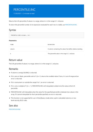


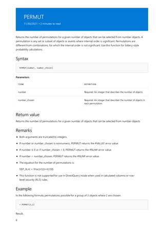
![RANK.EQ
11/30/2021 • 2 minutes to read
Syntax
RANK.EQ(<value>, <columnName>[, <order>])
Parameters
TERM DEFINITION
value Any DAX expression that returns a single scalar value whose
rank is to be found. The expression is to be evaluated exactly
once, before the function is evaluated, and it's value passed
to the argument list.
columnName The name of an existing column against which ranks will be
determined. It cannot be an expression or a column created
using these functions: ADDCOLUMNS, ROW or
SUMMARIZE.
order (Optional) A value that specifies how to rank number, low to
high or high to low:
order values
VALUE ALTERNATE VALUE DESCRIPTION
0 (zero) FALSE Ranks in descending order of
columnName. If value is equal to the
highest number in columnName then
RANK.EQ is 1.
1 TRUE Ranks in ascending order of
columnName. If value is equal to the
lowest number in columnName then
RANK.EQ is 1.
Return value
Remarks
Returns the ranking of a number in a list of numbers.
A number indicating the rank of value among the numbers in columnName.
columnName cannot refer to any column created using these functions: ADDCOLUMNS, ROW or
SUMMARIZE.I
If value is not in columnName or value is a blank, then RANK.EQ returns a blank value.
Duplicate values of value receive the same rank value; the next rank value assigned will be the rank value](https://image.slidesharecdn.com/funcoesdax-220812141017-bb6cd4dc/85/Funcoes-DAX-pdf-483-320.jpg)
![Example 1
= RANK.EQ(InternetSales_USD[SalesAmount_USD], InternetSales_USD[SalesAmount_USD])
Example 2
= RANK.EQ(Students[Test_Score], NationalScores[Test_Score])
plus the number of duplicate values. For example if five (5) values are tied with a rank of 11 then the next
value will receive a rank of 16 (11 + 5).
This function is not supported for use in DirectQuery mode when used in calculated columns or row-
level security (RLS) rules.
The following example creates a calculated column that ranks the values in SalesAmount_USD, from the
InternetSales_USD table, against all numbers in the same column.
The following example ranks a subset of values against a given sample. Assume that you have a table of local
students with their performance in a specific national test and, also, you have the entire set of scores in that
national test. The following calculated column will give you the national ranking for each of the local students.](https://image.slidesharecdn.com/funcoesdax-220812141017-bb6cd4dc/85/Funcoes-DAX-pdf-484-320.jpg)
![RANKX
11/30/2021 • 2 minutes to read
Syntax
RANKX(<table>, <expression>[, <value>[, <order>[, <ties>]]])
Parameters
VALUE ALTERNATE VALUE DESCRIPTION
0 (zero) FALSE Ranks in descending order of values of
expression. If value is equal to the
highest number in expression then
RANKX returns 1.
This is the default value when order
parameter is omitted.
1 TRUE Ranks in ascending order of
expression. If value is equal to the
lowest number in expression then
RANKX returns 1.
ENUMERATION DESCRIPTION
Returns the ranking of a number in a list of numbers for each row in the table argument.
table
Any DAX expression that returns a table of data over which the expression is evaluated.
expression
Any DAX expression that returns a single scalar value. The expression is evaluated for each row of table, to
generate all possible values for ranking. See the remarks section to understand the function behavior when
expression evaluates to BLANK.
value
(Optional) Any DAX expression that returns a single scalar value whose rank is to be found. See the remarks
section to understand the function's behavior when value is not found in the expression.
When the value parameter is omitted, the value of expression at the current row is used instead.
order
(Optional) A value that specifies how to rank value, low to high or high to low:
ties
(Optional) An enumeration that defines how to determine ranking when there are ties.](https://image.slidesharecdn.com/funcoesdax-220812141017-bb6cd4dc/85/Funcoes-DAX-pdf-485-320.jpg)
![Skip The next rank value, after a tie, is the rank value of the tie
plus the count of tied values. For example if five (5) values
are tied with a rank of 11 then the next value will receive a
rank of 16 (11 + 5).
This is the default value when ties parameter is omitted.
Dense The next rank value, after a tie, is the next rank value. For
example if five (5) values are tied with a rank of 11 then the
next value will receive a rank of 12.
ENUMERATION DESCRIPTION
Return value
Remarks
Example
= RANKX(ALL(Products), SUMX(RELATEDTABLE(InternetSales), [SalesAmount]))
The rank number of value among all possible values of expression evaluated for all rows of table numbers.
If expression or value evaluates to BLANK it is treated as a 0 (zero) for all expressions that result in a
number, or as an empty text for all text expressions.
If value is not among all possible values of expression then RANKX temporarily adds value to the values
from expression and re-evaluates RANKX to determine the proper rank of value.
Optional arguments might be skipped by placing an empty comma (,) in the argument list, i.e.
RANKX(Inventory, [InventoryCost],,,"Dense")
This function is not supported for use in DirectQuery mode when used in calculated columns or row-
level security (RLS) rules.
The following calculated column in the Products table calculates the sales ranking for each product in the
Internet channel.](https://image.slidesharecdn.com/funcoesdax-220812141017-bb6cd4dc/85/Funcoes-DAX-pdf-486-320.jpg)
![SAMPLE
11/30/2021 • 2 minutes to read
Syntax
SAMPLE(<n_value>, <table>, <orderBy_expression>, [<order>[, <orderBy_expression>, [<order>]]…])
Parameters
TERM DEFINITION
n_value The number of rows to return. It is any DAX expression that
returns a single scalar value, where the expression is to be
evaluated multiple times (for each row/context). If a non-
integer value (or expression) is entered, the result is cast as
an integer.
table Any DAX expression that returns a table of data from where
to extract the 'n' sample rows.
orderBy_expression (Optional) Any scalar DAX expression where the result value
is evaluated for each row of table.
order (Optional) A value that specifies how to sort
orderBy_expression values, ascending or descending: 0
(zero), sorts in descending order of values of order_by. 1,
ranks in ascending order of order_by.
Return value
Remarks
Returns a sample of N rows from the specified table.
A table consisting of a sample of N rows of table or an empty table if n_value is 0 (zero) or less. If OrderBy
arguments are provided, the sample will be stable and deterministic, returning the first row, the last row, and
evenly distributed rows between them. If no ordering is specified, the sample will be random, not stable, and not
deterministic.
If n_value is 0 (zero) or less then SAMPLE returns an empty table.
In order to avoid duplicate values in the sample, the table provided as the second argument should be
grouped by the column used for sorting.
This function is not supported for use in DirectQuery mode when used in calculated columns or row-
level security (RLS) rules.](https://image.slidesharecdn.com/funcoesdax-220812141017-bb6cd4dc/85/Funcoes-DAX-pdf-487-320.jpg)
![STDEV.S
11/30/2021 • 2 minutes to read
Syntax
STDEV.S(<ColumnName>)
Parameters
TERM DEFINITION
columnName The name of an existing column using standard DAX syntax,
usually fully qualified. It cannot be an expression.
Return value
Exceptions
Remarks
Example
= STDEV.S(InternetSales_USD[SalesAmount_USD])
Returns the standard deviation of a sample population.
A number that represents the standard deviation of a sample population.
STDEV.S assumes that the column refers to a sample of the population. If your data represents the entire
population, then compute the standard deviation by using STDEV.P.
STDEV.S uses the following formula:
Ã[∑(x - x̃) /(n-1)]
2
where x̃ is the average value of x for the sample population and n is the population size.
Blank rows are filtered out from columnName and not considered in the calculations.
An error is returned if columnName contains less than 2 non-blank rows.
This function is not supported for use in DirectQuery mode when used in calculated columns or row-
level security (RLS) rules.
The following example shows the formula for a measure that calculates the standard deviation of the column,
SalesAmount_USD, when the table InternetSales_USD is the sample population.](https://image.slidesharecdn.com/funcoesdax-220812141017-bb6cd4dc/85/Funcoes-DAX-pdf-488-320.jpg)
![STDEV.P
11/30/2021 • 2 minutes to read
Syntax
STDEV.P(<ColumnName>)
Parameters
TERM DEFINITION
columnName The name of an existing column using standard DAX syntax,
usually fully qualified. It cannot be an expression.
Return value
Remarks
Example
= STDEV.P(InternetSales_USD[SalesAmount_USD])
Returns the standard deviation of the entire population.
A number representing the standard deviation of the entire population.
STDEV.P assumes that the column refers to the entire population. If your data represents a sample of the
population, then compute the standard deviation by using STDEV.S.
STDEV.P uses the following formula:
Ã[∑(x - x̃) /n]
2
where x̃ is the average value of x for the entire population and n is the population size.
Blank rows are filtered out from columnName and not considered in the calculations.
An error is returned if columnName contains less than 2 non-blank rows
This function is not supported for use in DirectQuery mode when used in calculated columns or row-
level security (RLS) rules.
The following example shows the formula for a measure that calculates the standard deviation of the column,
SalesAmount_USD, when the table InternetSales_USD is the entire population.](https://image.slidesharecdn.com/funcoesdax-220812141017-bb6cd4dc/85/Funcoes-DAX-pdf-489-320.jpg)
![STDEVX.S
11/30/2021 • 2 minutes to read
Syntax
STDEVX.S(<table>, <expression>)
Parameters
TERM DEFINITION
table Any DAX expression that returns a single scalar value, where
the expression is to be evaluated multiple times (for each
row/context).
expression Any DAX expression that returns a single scalar value, where
the expression is to be evaluated multiple times (for each
row/context).
Return value
Exceptions
Remarks
Example
Returns the standard deviation of a sample population.
A number with the standard deviation of a sample population.
STDEVX.S evaluates expression for each row of table and returns the standard deviation of expression
assuming that table refers to a sample of the population. If table represents the entire population, then
compute the standard deviation by using STDEVX.P.
STDEVX.S uses the following formula:
Ã[∑(x - x̃) /(n-1)]
2
where x̃ is the average value of x for the entire population and n is the population size.
Blank rows are filtered out from columnName and not considered in the calculations.
An error is returned if columnName contains less than 2 non-blank rows.
This function is not supported for use in DirectQuery mode when used in calculated columns or row-
level security (RLS) rules.
The following example shows the formula for a calculated column that estimates the standard deviation of the
unit price per product for a sample population, when the formula is used in the Product table.](https://image.slidesharecdn.com/funcoesdax-220812141017-bb6cd4dc/85/Funcoes-DAX-pdf-490-320.jpg)
![= STDEVX.S(RELATEDTABLE(InternetSales_USD), InternetSales_USD[UnitPrice_USD] –
(InternetSales_USD[DiscountAmount_USD]/InternetSales_USD[OrderQuantity]))](https://image.slidesharecdn.com/funcoesdax-220812141017-bb6cd4dc/85/Funcoes-DAX-pdf-491-320.jpg)
![STDEVX.P
11/30/2021 • 2 minutes to read
Syntax
STDEVX.P(<table>, <expression>)
Parameters
TERM DEFINITION
table Any DAX expression that returns a single scalar value, where
the expression is to be evaluated multiple times (for each
row/context).
expression Any DAX expression that returns a single scalar value, where
the expression is to be evaluated multiple times (for each
row/context).
Return value
Remarks
Example
= STDEVX.P(RELATEDTABLE(InternetSales_USD), InternetSales_USD[UnitPrice_USD] –
(InternetSales_USD[DiscountAmount_USD]/InternetSales_USD[OrderQuantity]))
Returns the standard deviation of the entire population.
A number that represents the standard deviation of the entire population.
STDEVX.P evaluates expression for each row of table and returns the standard deviation of expression
assuming that table refers to the entire population. If the data in table represents a sample of the
population, you should compute the standard deviation by using STDEVX.S instead.
STDEVX.P uses the following formula:
Ã[∑(x - x̃) /n]
2
where x̃ is the average value of x for the entire population and n is the population size.
Blank rows are filtered out from columnName and not considered in the calculations.
An error is returned if columnName contains less than 2 non-blank rows
This function is not supported for use in DirectQuery mode when used in calculated columns or row-
level security (RLS) rules.
The following example shows the formula for a calculated column that calculates the standard deviation of the
unit price per product, when the formula is used in the Product table.](https://image.slidesharecdn.com/funcoesdax-220812141017-bb6cd4dc/85/Funcoes-DAX-pdf-492-320.jpg)
![T.DIST
11/30/2021 • 2 minutes to read
Syntax
T.DIST(X,Deg_freedom,Cumulative)
Parameters
TERM DEFINITION
X The numeric value at which to evaluate the distribution.
Deg_freedom An integer indicating the number of degrees of freedom.
Cumulative A logical value that determines the form of the function. If
cumulative is TRUE, T.DIST returns the cumulative
distribution function; if FALSE, it returns the probability
density function.
Return value
Remarks
Example
EVALUATE { T.DIST(60, 1, TRUE) }
[VALUE]
0.994695326367377
See also
Returns the Student's left-tailed t-distribution.
The Student's left-tailed t-distribution.
This function is not supported for use in DirectQuery mode when used in calculated columns or row-level
security (RLS) rules.
Returns,
T.DIST.2T
T.DIST.RT
T.INV
T.INV.2t](https://image.slidesharecdn.com/funcoesdax-220812141017-bb6cd4dc/85/Funcoes-DAX-pdf-493-320.jpg)
![T.DIST.2T
11/30/2021 • 2 minutes to read
Syntax
T.DIST.2T(X,Deg_freedom)
Parameters
TERM DEFINITION
X The numeric value at which to evaluate the distribution.
Deg_freedom An integer indicating the number of degrees of freedom.
Return value
Remarks
Example
EVALUATE { T.DIST.2T(1.959999998, 60) }
[VALUE]
0.054644929975921
See also
Returns the two-tailed Student's t-distribution.
The two-tailed Student's t-distribution.
This function is not supported for use in DirectQuery mode when used in calculated columns or row-level
security (RLS) rules.
Returns
T.DIST
T.DIST.RT
T.INV
T.INV.2t](https://image.slidesharecdn.com/funcoesdax-220812141017-bb6cd4dc/85/Funcoes-DAX-pdf-494-320.jpg)
![T.DIST.RT
11/30/2021 • 2 minutes to read
Syntax
T.DIST.RT(X,Deg_freedom)
Parameters
TERM DEFINITION
X The numeric value at which to evaluate the distribution.
Deg_freedom An integer indicating the number of degrees of freedom.
Return value
Remarks
Example
EVALUATE { T.DIST.RT(1.959999998, 60) }
[VALUE]
0.0273224649879605
See also
Returns the right-tailed Student's t-distribution.
The right-tailed Student's t-distribution.
This function is not supported for use in DirectQuery mode when used in calculated columns or row-level
security (RLS) rules.
Returns
T.DIST
T.DIST.2T
T.INV
T.INV.2t](https://image.slidesharecdn.com/funcoesdax-220812141017-bb6cd4dc/85/Funcoes-DAX-pdf-495-320.jpg)
![T.INV
11/30/2021 • 2 minutes to read
Syntax
T.INV(Probability,Deg_freedom)
Parameters
TERM DEFINITION
Probability The probability associated with the Student's t-distribution.
Deg_freedom The number of degrees of freedom with which to
characterize the distribution.
Return value
Remarks
Example
EVALUATE { T.INV(0.75, 2) }
[VALUE]
0.816496580927726
See also
Returns the left-tailed inverse of the Student's t-distribution.
The left-tailed inverse of the Student's t-distribution.
This function is not supported for use in DirectQuery mode when used in calculated columns or row-level
security (RLS) rules.
Returns
T.INV.2T
T.DIST
T.DIST.2T
T.DIST.RT](https://image.slidesharecdn.com/funcoesdax-220812141017-bb6cd4dc/85/Funcoes-DAX-pdf-496-320.jpg)
![T.INV.2T
11/30/2021 • 2 minutes to read
Syntax
T.INV.2T(Probability,Deg_freedom)
Parameters
TERM DEFINITION
Probability The probability associated with the Student's t-distribution.
Deg_freedom The number of degrees of freedom with which to
characterize the distribution.
Return value
Remarks
Example
EVALUATE { T.INV.2T(0.546449, 60) }
[VALUE]
0.606533075825759
See also
Returns the two-tailed inverse of the Student's t-distribution.
The two-tailed inverse of the Student's t-distribution.
This function is not supported for use in DirectQuery mode when used in calculated columns or row-level
security (RLS) rules.
Returns
T.INV
T.DIST
T.DIST.2T
T.DIST.RT](https://image.slidesharecdn.com/funcoesdax-220812141017-bb6cd4dc/85/Funcoes-DAX-pdf-497-320.jpg)
![VAR.S
11/30/2021 • 2 minutes to read
Syntax
VAR.S(<columnName>)
Parameters
TERM DEFINITION
columnName The name of an existing column using standard DAX syntax,
usually fully qualified. It cannot be an expression.
Return value
Remarks
Example
= VAR.S(InternetSales_USD[SalesAmount_USD])
Returns the variance of a sample population.
A number with the variance of a sample population.
VAR.S assumes that the column refers to a sample of the population. If your data represents the entire
population, then compute the variance by using VAR.P.
VAR.S uses the following formula:
∑(x - x̃) /(n-1)
2
where x̃ is the average value of x for the sample population
and n is the population size
Blank rows are filtered out from columnName and not considered in the calculations.
An error is returned if columnName contains less than 2 non-blank rows.
This function is not supported for use in DirectQuery mode when used in calculated columns or row-
level security (RLS) rules.
The following example shows the formula for a measure that calculates the variance of the SalesAmount_USD
column from the InternetSales_USD for a sample population.](https://image.slidesharecdn.com/funcoesdax-220812141017-bb6cd4dc/85/Funcoes-DAX-pdf-498-320.jpg)
![VAR.P
11/30/2021 • 2 minutes to read
Syntax
VAR.P(<columnName>)
Parameters
TERM DEFINITION
columnName The name of an existing column using standard DAX syntax,
usually fully qualified. It cannot be an expression.
Return value
Remarks
Example
= VAR.P(InternetSales_USD[SalesAmount_USD])
Returns the variance of the entire population.
A number with the variance of the entire population.
VAR.P assumes that the column refers the entire population. If your data represents a sample of the
population, then compute the variance by using VAR.S.
VAR.P uses the following formula:
∑(x - x̃) /n
2
where x̃ is the average value of x for the entire population
and n is the population size
Blank rows are filtered out from columnName and not considered in the calculations.
An error is returned if columnName contains less than 2 non-blank rows
This function is not supported for use in DirectQuery mode when used in calculated columns or row-
level security (RLS) rules.
The following example shows the formula for a measure that estimates the variance of the SalesAmount_USD
column from the InternetSales_USD table, for the entire population.](https://image.slidesharecdn.com/funcoesdax-220812141017-bb6cd4dc/85/Funcoes-DAX-pdf-499-320.jpg)
![VARX.S
11/30/2021 • 2 minutes to read
Syntax
VARX.S(<table>, <expression>)
Parameters
TERM DEFINITION
table Any DAX expression that returns a table of data.
expression Any DAX expression that returns a single scalar value, where
the expression is to be evaluated multiple times (for each
row/context).
Return value
Remarks
Example
= VARX.S(InternetSales_USD, InternetSales_USD[UnitPrice_USD] –
(InternetSales_USD[DiscountAmount_USD]/InternetSales_USD[OrderQuantity]))
Returns the variance of a sample population.
A number that represents the variance of a sample population.
VARX.S evaluates expression for each row of table and returns the variance of expression; on the
assumption that table refers to a sample of the population. If table represents the entire population, then
you should compute the variance by using VARX.P.
VAR.S uses the following formula:
∑(x - x̃) /(n-1)
2
where x̃ is the average value of x for the sample population
and n is the population size
Blank rows are filtered out from columnName and not considered in the calculations.
An error is returned if columnName contains less than 2 non-blank rows.
This function is not supported for use in DirectQuery mode when used in calculated columns or row-
level security (RLS) rules.
The following example shows the formula for a calculated column that estimates the variance of the unit price
per product for a sample population, when the formula is used in the Product table.](https://image.slidesharecdn.com/funcoesdax-220812141017-bb6cd4dc/85/Funcoes-DAX-pdf-500-320.jpg)
![VARX.P
11/30/2021 • 2 minutes to read
Syntax
VARX.P(<table>, <expression>)
Parameters
TERM DEFINITION
table Any DAX expression that returns a table of data.
expression Any DAX expression that returns a single scalar value, where
the expression is to be evaluated multiple times (for each
row/context).
Return value
Remarks
Example
= VARX.P(InternetSales_USD, InternetSales_USD[UnitPrice_USD] –
(InternetSales_USD[DiscountAmount_USD]/InternetSales_USD[OrderQuantity]))
Returns the variance of the entire population.
A number with the variance of the entire population.
VARX.P evaluates <expression> for each row of <table> and returns the variance of <expression>
assuming that <table> refers to the entire population.. If <table> represents a sample of the population,
then compute the variance by using VARX.S.
VARX.P uses the following formula:
∑(x - x̃) /n
2
where x̃ is the average value of x for the entire population
and n is the population size
Blank rows are filtered out from columnName and not considered in the calculations.
An error is returned if columnName contains less than 2 non-blank rows
This function is not supported for use in DirectQuery mode when used in calculated columns or row-
level security (RLS) rules.
The following example shows the formula for a calculated column that calculates the variance of the unit price
per product, when the formula is used in the Product table](https://image.slidesharecdn.com/funcoesdax-220812141017-bb6cd4dc/85/Funcoes-DAX-pdf-501-320.jpg)
![ADDCOLUMNS
11/30/2021 • 2 minutes to read
Syntax
ADDCOLUMNS(<table>, <name>, <expression>[, <name>, <expression>]…)
Parameters
TERM DEFINITION
table Any DAX expression that returns a table of data.
name The name given to the column, enclosed in double quotes.
expression Any DAX expression that returns a scalar expression,
evaluated for each row of table.
Return value
Remarks
Example
ADDCOLUMNS(ProductCategory,
, "Internet Sales", SUMX(RELATEDTABLE(InternetSales_USD), InternetSales_USD[SalesAmount_USD])
, "Reseller Sales", SUMX(RELATEDTABLE(ResellerSales_USD),
ResellerSales_USD[SalesAmount_USD]))
PRODUCTCATEGORY[
PRODUCTCATEGORY
NAME]
PRODUCTCATEGORY[
PRODUCTCATEGORY
ALTERNATEKEY]
PRODUCTCATEGORY[
PRODUCTCATEGORY
KEY] [INTERNET SALES] [RESELLER SALES]
Bikes 1 1 25107749.77 63084675.04
Components 2 2 11205837.96
Adds calculated columns to the given table or table expression.
A table with all its original columns and the added ones.
This function is not supported for use in DirectQuery mode when used in calculated columns or row-level
security (RLS) rules.
The following example returns an extended version of the Product Category table that includes total sales values
from the reseller channel and the internet sales.
The following table shows a preview of the data as it would be received by any function expecting to receive a
table:](https://image.slidesharecdn.com/funcoesdax-220812141017-bb6cd4dc/85/Funcoes-DAX-pdf-505-320.jpg)
![Clothing 3 3 306157.5829 1669943.267
Accessories 4 4 640920.1338 534301.9888
PRODUCTCATEGORY[
PRODUCTCATEGORY
NAME]
PRODUCTCATEGORY[
PRODUCTCATEGORY
ALTERNATEKEY]
PRODUCTCATEGORY[
PRODUCTCATEGORY
KEY] [INTERNET SALES] [RESELLER SALES]](https://image.slidesharecdn.com/funcoesdax-220812141017-bb6cd4dc/85/Funcoes-DAX-pdf-506-320.jpg)
![ADDMISSINGITEMS
11/30/2021 • 2 minutes to read
Syntax
ADDMISSINGITEMS ( [<showAll_columnName> [, <showAll_columnName> [, … ] ] ], <table> [, <groupBy_columnName>
[, [<filterTable>] [, <groupBy_columnName> [, [<filterTable>] [, … ] ] ] ] ] ] )
Parameters
TERM DEFINITION
showAll_columnName (Optional) A column for which to return items with no data
for the measures used. If not specified, all columns are
returned.
table A SUMMARIZECOLUMNS table.
groupBy_columnName (Optional) A column to group by in the supplied table
argument.
filterTable (Optional) A table expression that defines which rows are
returned.
Return value
Remarks
With SUMMARIZECOLUMNS
Example
SUMMARIZECOLUMNS(
'Sales'[CustomerId],
"Total Qty", SUM ( Sales[TotalQty] )
)
Adds rows with empty values to a table returned by SUMMARIZECOLUMNS.
A table with one or more columns.
This function is not supported for use in DirectQuery mode when used in calculated columns or row-level
security (RLS) rules.
A table returned by SUMMARIZECOLUMNS will include only rows with values. By wrapping a
SUMMARIZECOLUMNS expression within an ADDMISSINGITEMS expression, rows containing no values are
also returned.
Without ADDMISSINGITEMS, the following query:
Returns,](https://image.slidesharecdn.com/funcoesdax-220812141017-bb6cd4dc/85/Funcoes-DAX-pdf-507-320.jpg)
![CUSTOMERID TOTALQTY
A 5
B 3
C 3
E 2
EVALUATE
ADMISSINGITEMS (
'Sales'[CustomerId],
SUMMARIZECOLUMNS(
'Sales'[CustomerId],
"Total Qty", SUM ( Sales[TotalQty] )
),
'Sales'[CustomerId]
)
CUSTOMERID TOTALQTY
A 5
B 3
C 3
D
E 2
F
With ADDMISSINGITEMS, the following query:
Returns,](https://image.slidesharecdn.com/funcoesdax-220812141017-bb6cd4dc/85/Funcoes-DAX-pdf-508-320.jpg)
![CROSSJOIN
11/30/2021 • 2 minutes to read
Syntax
CROSSJOIN(<table>, <table>[, <table>]…)
Parameters
TERM DEFINITION
table Any DAX expression that returns a table of data
Return value
Remarks
Example
COLOR PATTERN
Red Horizontal Stripe
Green Vertical Stripe
Blue Crosshatch
Returns a table that contains the Cartesian product of all rows from all tables in the arguments. The columns in
the new table are all the columns in all the argument tables.
A table that contains the Cartesian product of all rows from all tables in the arguments.
Column names from table arguments must all be different in all tables or an error is returned.
The total number of rows returned by CROSSJOIN() is equal to the product of the number of rows from
all tables in the arguments; also, the total number of columns in the result table is the sum of the number
of columns in all tables. For example, if TableA has rA rows and cA columns, and TableB has rB rows
and cB columns, and TableC has rC rows and cC column; then, the resulting table has rA × rb × rC
rows and cA + cB + cC columns.
This function is not supported for use in DirectQuery mode when used in calculated columns or row-
level security (RLS) rules.
The following example shows the results of applying CROSSJOIN() to two tables: Colors and Stationery.
The table Colors contains colors and patterns:
The table Stationery contains fonts and presentation:](https://image.slidesharecdn.com/funcoesdax-220812141017-bb6cd4dc/85/Funcoes-DAX-pdf-509-320.jpg)
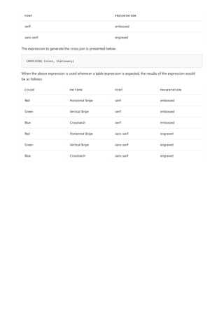
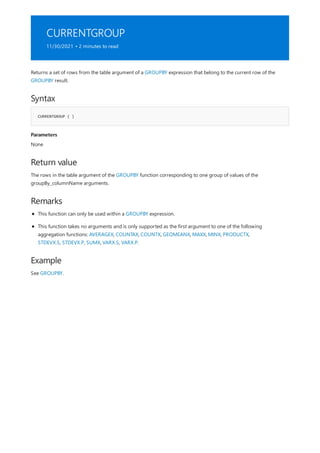
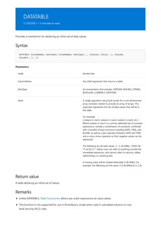
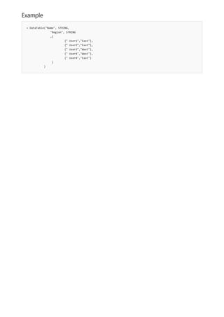
![DETAILROWS
11/30/2021 • 2 minutes to read
Syntax
DETAILROWS([Measure])
Parameters
TERM DEFINITION
Measure Name of a measure.
Return value
Evaluates a Detail Rows Expression defined for a measure and returns the data.
A table with the data returned by the Detail Rows Expression. If no Detail Rows Expression is defined, the data for
the table containing the measure is returned.](https://image.slidesharecdn.com/funcoesdax-220812141017-bb6cd4dc/85/Funcoes-DAX-pdf-514-320.jpg)
![= COUNTROWS(DISTINCT(InternetSales_USD[CustomerKey]))
ROW LABELS ACCESSORIES BIKES CLOTHING GRAND TOTAL
2005 1013 1013
2006 2677 2677
2007 6792 4875 2867 9309
2008 9435 5451 4196 11377
Grand Total 15114 9132 6852 18484
See also
You cannot paste the list of values that DISTINCT returns directly into a column. Instead, you pass the results of
the DISTINCT function to another function that counts, filters, or aggregates values by using the list. To make the
example as simple as possible, here the table of distinct values has been passed to the COUNTROWS function.
Also, note that the results are not additive. That is to say, the total number of unique customers in 2007 is not
the sum of unique customers of Accessories, Bikes and Clothing for that year. The reason is that a customer can
be counted in multiple groups.
Filter functions
FILTER function
RELATED function
VALUES function](https://image.slidesharecdn.com/funcoesdax-220812141017-bb6cd4dc/85/Funcoes-DAX-pdf-516-320.jpg)
![DISTINCT (table)
11/30/2021 • 2 minutes to read
Syntax
DISTINCT(<table>)
Parameters
TERM DEFINITION
table The table from which unique rows are to be returned. The
table can also be an expression that results in a table.
Return value
Related functions
Example
EVALUATE DISTINCT( { (1, "A"), (2, "B"), (1, "A") } )
[VALUE1] [VALUE2]
1 A
2 B
See also
Returns a table by removing duplicate rows from another table or expression.
A table containing only distinct rows.
There is another version of the DISTINCT function, DISTINCT (column), that takes a column name as input
parameter.
The following query:
Returns table:
Filter functions
DISTINCT (column)
FILTER function
RELATED function
VALUES function](https://image.slidesharecdn.com/funcoesdax-220812141017-bb6cd4dc/85/Funcoes-DAX-pdf-517-320.jpg)
![FILTERS
11/30/2021 • 2 minutes to read
Syntax
FILTERS(<columnName>)
Parameters
TERM DESCRIPTION
columnName The name of an existing column, using standard DAX syntax.
It cannot be an expression.
Return value
Remarks
Example
= COUNTROWS(FILTERS(ResellerSales_USD[ProductKey]))
Returns the values that are directly applied as filters to columnName.
The values that are directly applied as filters to columnName.
This function is not supported for use in DirectQuery mode when used in calculated columns or row-level
security (RLS) rules.
The following example shows how to determine the number of direct filters a column has.
This example lets you know how many direct filters on ResellerSales_USD[ProductKey] have been applied to the
context where the expression is being evaluated.](https://image.slidesharecdn.com/funcoesdax-220812141017-bb6cd4dc/85/Funcoes-DAX-pdf-520-320.jpg)
![GENERATE
11/30/2021 • 2 minutes to read
Syntax
GENERATE(<table1>, <table2>)
Parameters
TERM DEFINITION
table1 Any DAX expression that returns a table.
table2 Any DAX expression that returns a table.
Return value
Remarks
Example
SALESTERRITORY[SALESTERRITORYGR
OUP]
PRODUCTCATEGORY[PRODUCTCATEG
ORYNAME] [RESELLER SALES]
Europe Accessories $ 142,227.27
Europe Bikes $ 9,970,200.44
Europe Clothing $ 365,847.63
Returns a table with the Cartesian product between each row in table1 and the table that results from evaluating
table2 in the context of the current row from table1.
A table with the Cartesian product between each row in table1 and the table that results from evaluating table2
in the context of the current row from table1
If the evaluation of table2 for the current row in table1 returns an empty table, then the result table will
not contain the current row from table1. This is different than GENERATEALL() where the current row
from table1 will be included in the results and columns corresponding to table2 will have null values for
that row.
All column names from table1 and table2 must be different or an error is returned.
This function is not supported for use in DirectQuery mode when used in calculated columns or row-
level security (RLS) rules.
In the following example the user wants a summary table of the sales by Region and Product Category for the
Resellers channel, like the following table:](https://image.slidesharecdn.com/funcoesdax-220812141017-bb6cd4dc/85/Funcoes-DAX-pdf-521-320.jpg)
![Europe Components $ 2,214,440.19
North America Accessories $ 379,305.15
North America Bikes $ 52,403,796.85
North America Clothing $ 1,281,193.26
North America Components $ 8,882,848.05
Pacific Accessories $ 12,769.57
Pacific Bikes $ 710,677.75
Pacific Clothing $ 22,902.38
Pacific Components $ 108,549.71
SALESTERRITORY[SALESTERRITORYGR
OUP]
PRODUCTCATEGORY[PRODUCTCATEG
ORYNAME] [RESELLER SALES]
GENERATE(
SUMMARIZE(SalesTerritory, SalesTerritory[SalesTerritoryGroup])
,SUMMARIZE(ProductCategory
, [ProductCategoryName]
, "Reseller Sales", SUMX(RELATEDTABLE(ResellerSales_USD), ResellerSales_USD[SalesAmount_USD])
)
)
The following formula produces the above table:
SALESTERRITORY[SALESTERRITORYGROUP]
North America
Europe
Pacific
NA
PRODUCTCATEGORY[PRODUCTCATEGORYNAME] [RESELLER SALES]
Bikes $ 63,084,675.04
Components $ 11,205,837.96
1. The first SUMMARIZE statement, SUMMARIZE(SalesTerritory, SalesTerritory[SalesTerritoryGroup]) ,
produces a table of territory groups, where each row is a territory group, as shown below:
2. The second SUMMARIZE statement,
SUMMARIZE(ProductCategory, [ProductCategoryName], "Reseller Sales",
SUMX(RELATEDTABLE(ResellerSales_USD), ResellerSales_USD[SalesAmount_USD]))
, produces a table of Product Category groups with the Reseller sales for each group, as shown below:](https://image.slidesharecdn.com/funcoesdax-220812141017-bb6cd4dc/85/Funcoes-DAX-pdf-522-320.jpg)
![Clothing $ 1,669,943.27
Accessories $ 534,301.99
PRODUCTCATEGORY[PRODUCTCATEGORYNAME] [RESELLER SALES]
3. However, when you take the above table and evaluate it under the context of each row from the territory
groups table, you obtain different results for each territory.](https://image.slidesharecdn.com/funcoesdax-220812141017-bb6cd4dc/85/Funcoes-DAX-pdf-523-320.jpg)
![GENERATEALL
11/30/2021 • 2 minutes to read
Syntax
GENERATEALL(<table1>, <table2>)
Parameters
TERM DEFINITION
table1 Any DAX expression that returns a table.
table2 Any DAX expression that returns a table.
Return value
Remarks
Example
SALESTERRITORY[SALESTERRITORYGR
OUP]
PRODUCTCATEGORY[PRODUCTCATEG
ORYNAME] [RESELLER SALES]
Europe Accessories $ 142,227.27
Europe Bikes $ 9,970,200.44
Europe Clothing $ 365,847.63
Returns a table with the Cartesian product between each row in table1 and the table that results from evaluating
table2 in the context of the current row from table1.
A table with the Cartesian product between each row in table1 and the table that results from evaluating table2
in the context of the current row from table1
If the evaluation of table2 for the current row in table1 returns an empty table, then the current row from
table1 will be included in the results and columns corresponding to table2 will have null values for that
row. This is different than GENERATE() where the current row from table1 will not be included in the
results.
All column names from table1 and table2 must be different or an error is returned.
This function is not supported for use in DirectQuery mode when used in calculated columns or row-
level security (RLS) rules.
In the following example, the user wants a summary table of the sales by Region and Product Category for the
Resellers channel, like the following table:](https://image.slidesharecdn.com/funcoesdax-220812141017-bb6cd4dc/85/Funcoes-DAX-pdf-524-320.jpg)
![Europe Components $ 2,214,440.19
NA Accessories
NA Bikes
NA Clothing
NA Components
North America Accessories $ 379,305.15
North America Bikes $ 52,403,796.85
North America Clothing $ 1,281,193.26
North America Components $ 8,882,848.05
Pacific Accessories $ 12,769.57
Pacific Bikes $ 710,677.75
Pacific Clothing $ 22,902.38
Pacific Components $ 108,549.71
SALESTERRITORY[SALESTERRITORYGR
OUP]
PRODUCTCATEGORY[PRODUCTCATEG
ORYNAME] [RESELLER SALES]
GENERATEALL(
SUMMARIZE(SalesTerritory, SalesTerritory[SalesTerritoryGroup])
,SUMMARIZE(ProductCategory
, [ProductCategoryName]
, "Reseller Sales", SUMX(RELATEDTABLE(ResellerSales_USD), ResellerSales_USD[SalesAmount_USD])
)
)
The following formula produces the above table:
SALESTERRITORY[SALESTERRITORYGROUP]
North America
Europe
Pacific
NA
1. The first SUMMARIZE produces a table of territory groups, where each row is a territory group, like those
listed below:
2. The second SUMMARIZE produces a table of Product Category groups with the Reseller sales for each
group, as shown below:](https://image.slidesharecdn.com/funcoesdax-220812141017-bb6cd4dc/85/Funcoes-DAX-pdf-525-320.jpg)
![PRODUCTCATEGORY[PRODUCTCATEGORYNAME] [RESELLER SALES]
Bikes $ 63,084,675.04
Components $ 11,205,837.96
Clothing $ 1,669,943.27
Accessories $ 534,301.99
3. However, when you take the above table and evaluate the table under the context of each row from the
territory groups table, you obtain different results for each territory.](https://image.slidesharecdn.com/funcoesdax-220812141017-bb6cd4dc/85/Funcoes-DAX-pdf-526-320.jpg)
![GENERATESERIES
11/30/2021 • 2 minutes to read
Syntax
GENERATESERIES(<startValue>, <endValue>[, <incrementValue>])
Parameters
TERM DEFINITION
startValue The initial value used to generate the sequence.
endValue The end value used to generate the sequence.
incrementValue (Optional) The increment value of the sequence. When not
provided, the default value is 1.
Return value
Remarks
Example 1
EVALUATE GENERATESERIES(1, 5)
[VALUE]
1
2
Returns a single column table containing the values of an arithmetic series, that is, a sequence of values in which
each differs from the preceding by a constant quantity. The name of the column returned is Value.
A single column table containing the values of an arithmetic series. The name of the column is Value.
When startValue is less than endValue, an empty table is returned.
incrementValue must be a positive value.
The sequence stops at the last value that is less than or equal to endValue.
This function is not supported for use in DirectQuery mode when used in calculated columns or row-
level security (RLS) rules.
The following DAX query:
Returns the following table with a single column:](https://image.slidesharecdn.com/funcoesdax-220812141017-bb6cd4dc/85/Funcoes-DAX-pdf-527-320.jpg)
![3
4
5
[VALUE]
Example 2
EVALUATE GENERATESERIES(1.2, 2.4, 0.4)
[VALUE]
1.2
1.6
2
2.4
Example 3
EVALUATE GENERATESERIES(CURRENCY(10), CURRENCY(12.4), CURRENCY(0.5))
[VALUE]
10
10.5
11
11.5
12
The following DAX query:
Returns the following table with a single column:
The following DAX query:
Returns the following table with a single column:](https://image.slidesharecdn.com/funcoesdax-220812141017-bb6cd4dc/85/Funcoes-DAX-pdf-528-320.jpg)
![GROUPBY
11/30/2021 • 2 minutes to read
Syntax
GROUPBY (<table> [, <groupBy_columnName> [, <groupBy_columnName> [, …]]] [, <name>, <expression> [, <name>,
<expression> [, …]]])
Parameters
TERM DEFINITION
table Any DAX expression that returns a table of data.
groupBy_columnName The name of an existing column in the table (or in a related
table,) by which the data is to be grouped. This parameter
cannot be an expression.
name The name given to a new column that is being added to the
list of GroupBy columns, enclosed in double quotes.
expression One of the X aggregation functions with the first argument
being CURRENTGROUP(). See With CURRENTGROUP section
below for the full list of supported X aggregation functions.
Return value
Remarks
The GROUPBY function is similar to the SUMMARIZE function. However, GROUPBY does not do an implicit
CALCULATE for any extension columns that it adds. GROUPBY permits a new function, CURRENTGROUP, to be
used inside aggregation functions in the extension columns that it adds. GROUPBY is used to perform multiple
aggregations in a single table scan.
A table with the selected columns for the groupBy_columnName arguments and the extension columns
designated by the name arguments.
The GROUPBY function does the following:
1. Start with the specified table (and all related tables in the "to-one" direction).
2. Create a grouping using all of the GroupBy columns (which are required to exist in the table from
step #1.).
3. Each group is one row in the result, but represents a set of rows in the original table.
4. For each group, evaluate the extension columns being added. Unlike the SUMMARIZE function, an
implied CALCULATE is not performed, and the group isn't placed into the filter context.
Each column for which you define a name must have a corresponding expression; otherwise, an error is
returned. The first argument, name, defines the name of the column in the results. The second argument,
expression, defines the calculation performed to obtain the value for each row in that column.](https://image.slidesharecdn.com/funcoesdax-220812141017-bb6cd4dc/85/Funcoes-DAX-pdf-529-320.jpg)
![With CURRENTGROUP
Example
DEFINE
VAR SalesByCountryAndCategory =
SUMMARIZECOLUMNS(
Geography[Country],
Product[Category],
"Total Sales", SUMX(Sales, Sales[Price] * Sales[Qty])
)
EVALUATE
GROUPBY(
SalesByCountryAndCategory,
Geography[Country],
"Max Sales", MAXX(CURRENTGROUP(), [Total Sales])
)
See also
groupBy_columnName must be either in table or in a related table.
Each name must be enclosed in double quotation marks.
The function groups a selected set of rows into a set of summary rows by the values of one or more
groupBy_columnName columns. One row is returned for each group.
GROUPBY is primarily used to perform aggregations over intermediate results from DAX table
expressions. For efficient aggregations over physical tables in the model, consider using
SUMMARIZECOLUMNS or SUMMARIZE function.
This function is not supported for use in DirectQuery mode when used in calculated columns or row-
level security (RLS) rules.
CURRENTGROUP can only be used in an expression that defines an extension column within the GROUPBY
function. In-effect, CURRENTGROUP returns a set of rows from the table argument of GROUPBY that belong to
the current row of the GROUPBY result. The CURRENTGROUP function takes no arguments and is only
supported as the first argument to one of the following aggregation functions: AVERAGEX, COUNTAX, COUNTX,
GEOMEANX, MAXX, MINX, PRODUCTX, STDEVX.S, STDEVX.P, SUMX, VARX.S, VARX.P.
The following example first calculates the total sales grouped by country and product category over physical
tables by using the SUMMARIZECOLUMNS function. It then uses the GROUPBY function to scan the
intermediate result from the first step to find the maximum sales in each country across the product categories.
SUMMARIZE function
SUMMARIZECOLUMNS function](https://image.slidesharecdn.com/funcoesdax-220812141017-bb6cd4dc/85/Funcoes-DAX-pdf-530-320.jpg)
![IGNORE
11/30/2021 • 2 minutes to read
Syntax
IGNORE(<expression>)
SUMMARIZECOLUMNS(<groupBy_columnName>[, < groupBy_columnName >]…, [<filterTable>]…[, <name>, IGNORE(…)]…)
Parameters
TERM DEFINITION
expression Any DAX expression that returns a single value (not a table).
Return value
Remarks
Example
Modifies the behavior of the SUMMARIZECOLUMNS function by omitting specific expressions from the
BLANK/NULL evaluation. Rows for which all expressions not using IGNORE return BLANK/NULL will be
excluded independent of whether the expressions which do use IGNORE evaluate to BLANK/NULL or not. This
function can only be used within a SUMMARIZECOLUMNS expression.
With SUMMARIZECOLUMNS,
The function does not return a value.
IGNORE can only be used as an expression argument to SUMMARIZECOLUMNS.
See SUMMARIZECOLUMNS.](https://image.slidesharecdn.com/funcoesdax-220812141017-bb6cd4dc/85/Funcoes-DAX-pdf-531-320.jpg)
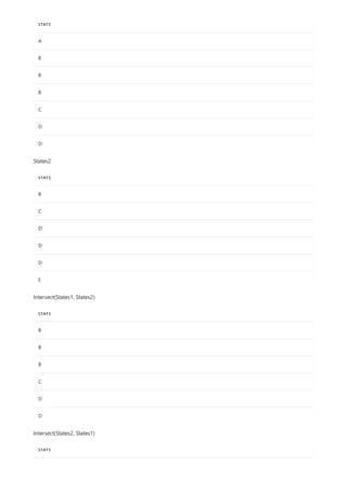
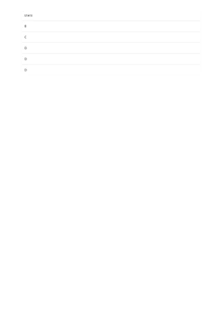
![NATURALINNERJOIN
11/30/2021 • 2 minutes to read
Syntax
NATURALINNERJOIN(<leftJoinTable>, <rightJoinTable>)
Parameters
TERM DEFINITION
leftJoinTable A table expression defining the table on the left side of the
join.
rightJoinTable A table expression defining the table on the right side of the
join.
Return value
Remarks
Performs an inner join of a table with another table. The tables are joined on common columns (by name) in the
two tables. If the two tables have no common column names, an error is returned.
A table which includes only rows for which the values in the common columns specified are present in both
tables. The table returned will have the common columns from the left table and other columns from both the
tables.
There is no sort order guarantee for the results.
Columns being joined on must have the same data type in both tables.
Only columns from the same source table (have the same lineage) are joined on. For example,
Products[ProductID], WebSales[ProductdID], StoreSales[ProductdID] with many-to-one relationships
between WebSales and StoreSales and the Products table based on the ProductID column, WebSales and
StoreSales tables are joined on [ProductID].
Strict comparison semantics are used during join. There is no type coercion; for example, 1 does not equal
1.0.
This function is not supported for use in DirectQuery mode when used in calculated columns or row-
level security (RLS) rules.](https://image.slidesharecdn.com/funcoesdax-220812141017-bb6cd4dc/85/Funcoes-DAX-pdf-535-320.jpg)
![NATURALLEFTOUTERJOIN
11/30/2021 • 2 minutes to read
Syntax
NATURALLEFTOUTERJOIN(<leftJoinTable>, <rightJoinTable>)
Parameters
TERM DEFINITION
leftJoinTable A table expression defining the table on the left side of the
join.
rightJoinTable A table expression defining the table on the right side of the
join.
Return value
Remarks
Performs an inner join of a table with another table. The tables are joined on common columns (by name) in the
two tables. If the two tables have no common column names, an error is returned.
A table which includes only rows from rightJoinTable for which the values in the common columns specified are
also present in leftJoinTable. The table returned will have the common columns from the left table and the other
columns from both the tables.
There is no sort order guarantee for the results.
Columns being joined on must have the same data type in both tables.
Only columns from the same source table (have the same lineage) are joined on. For example,
Products[ProductID], WebSales[ProductdID], StoreSales[ProductdID] with many-to-one relationships
between WebSales and StoreSales and the Products table based on the ProductID column, WebSales and
StoreSales tables are joined on [ProductID].
Strict comparison semantics are used during join. There is no type coercion; for example, 1 does not equal
1.0.
This function is not supported for use in DirectQuery mode when used in calculated columns or row-
level security (RLS) rules.](https://image.slidesharecdn.com/funcoesdax-220812141017-bb6cd4dc/85/Funcoes-DAX-pdf-536-320.jpg)
![ROLLUP
11/30/2021 • 2 minutes to read
Syntax
ROLLUP ( <groupBy_columnName> [, <groupBy_columnName> [, … ] ] )
SUMMARIZE(<table>, <groupBy_columnName>[, <groupBy_columnName>]…[, ROLLUP(<groupBy_columnName>[,<
groupBy_columnName>…])][, <name>, <expression>]…)
Parameters
TERM DEFINITION
groupBy_columnName The qualified name of an existing column or ROLLUPGROUP
function to be used to create summary groups based on the
values found in it. This parameter cannot be an expression.
Return value
Remarks
Example
Modifies the behavior of the SUMMARIZE function by adding rollup rows to the result on columns defined by
the groupBy_columnName parameter. This function can only be used within a SUMMARIZE expression.
With SUMMARIZE,
This function does not return a value. It only specifies the set of columns to be subtotaled.
This function can only be used within a SUMMARIZE expression.
See SUMMARIZE.](https://image.slidesharecdn.com/funcoesdax-220812141017-bb6cd4dc/85/Funcoes-DAX-pdf-537-320.jpg)
![ROLLUPADDISSUBTOTAL
11/30/2021 • 2 minutes to read
Syntax
ROLLUPADDISSUBTOTAL ( [<grandtotalFilter>], <groupBy_columnName>, <name> [, [<groupLevelFilter>] [,
<groupBy_columnName>, <name> [, [<groupLevelFilter>] [, … ] ] ] ] )
Parameters
TERM DEFINITION
grandtotalFilter (Optional) Filter to be applied to the grandtotal level.
groupBy_columnName Name of an existing column used to create summary groups
based on the values found in it. Cannot be an expression.
name Name of an ISSUBTOTAL column. The values of the column
are calculated using the ISSUBTOTAL function.
groupLevelFilter (Optional) Filter to be applied to the current level.
Return value
Remarks
Example
Modifies the behavior of the SUMMARIZECOLUMNS function by adding rollup/subtotal rows to the result based
on the groupBy_columnName columns. This function can only be used within a SUMMARIZECOLUMNS
expression.
The function does not return a value.
None
See SUMMARIZECOLUMNS.](https://image.slidesharecdn.com/funcoesdax-220812141017-bb6cd4dc/85/Funcoes-DAX-pdf-538-320.jpg)
![ROLLUPGROUP
11/30/2021 • 2 minutes to read
Syntax
ROLLUPGROUP ( <groupBy_columnName> [, <groupBy_columnName> [, … ] ] )
Parameters
TERM DEFINITION
groupBy_columnName The qualified name of an existing column or ROLLUPGROUP
function to be used to create summary groups based on the
values found in it. This parameter cannot be an expression.
Return value
Remarks
Example
Modifies the behavior of the SUMMARIZE and SUMMARIZECOLUMNS functions by adding rollup rows to the
result on columns defined by the the groupBy_columnName parameter. This function can only be used within a
SUMMARIZE or SUMMARIZECOLUMNS expression.
This function does not return a value. It marks a set of columns to be treated as a single group during
subtotaling by ROLLUP or ROLLUPADDISSUBTOTAL.
ROLLUPGROUP can only be used as a groupBy_columnName argument to ROLLUP, ROLLUPADDISSUBTOTAL,
or ROLLUPISSUBTOTAL.
See SUMMARIZE and SUMMARIZECOLUMNS.](https://image.slidesharecdn.com/funcoesdax-220812141017-bb6cd4dc/85/Funcoes-DAX-pdf-539-320.jpg)
![ROLLUPISSUBTOTAL
11/30/2021 • 2 minutes to read
Syntax
ROLLUPISSUBTOTAL ( [<grandTotalFilter>], <groupBy_columnName>, <isSubtotal_columnName> [,
[<groupLevelFilter>] [, <groupBy_columnName>, <isSubtotal_columnName> [, [<groupLevelFilter>] [, … ] ] ] ] )
Parameters
TERM DEFINITION
grandTotalFilter (Optional) Filter to be applied to the grandtotal level.
groupBy_columnName Name of an existing column used to create summary groups
based on the values found in it. Cannot be an expression.
isSubtotal_columnName Name of an ISSUBTOTAL column. The values of the column
are calculated using the ISSUBTOTAL function.
groupLevelFilter (Optional) Filter to be applied to the current level.
Return value
Remarks
Pairs rollup groups with the column added by ROLLUPADDISSUBTOTAL. This function can only be used within an
ADDMISSINGITEMS expression.
None
This function can only be used within an ADDMISSINGITEMS expression.](https://image.slidesharecdn.com/funcoesdax-220812141017-bb6cd4dc/85/Funcoes-DAX-pdf-540-320.jpg)
![ROW function
11/30/2021 • 2 minutes to read
Syntax
ROW(<name>, <expression>[[,<name>, <expression>]…])
Parameters
TERM DEFINITION
name The name given to the column, enclosed in double quotes.
expression Any DAX expression that returns a single scalar value to
populate. name.
Return value
Remarks
Example
ROW("Internet Total Sales (USD)", SUM(InternetSales_USD[SalesAmount_USD]),
"Resellers Total Sales (USD)", SUM(ResellerSales_USD[SalesAmount_USD]))
Returns a table with a single row containing values that result from the expressions given to each column.
A single row table
Arguments must always come in pairs of name and expression.
This function is not supported for use in DirectQuery mode when used in calculated columns or row-
level security (RLS) rules.
The following example returns a single row table with the total sales for internet and resellers channels.](https://image.slidesharecdn.com/funcoesdax-220812141017-bb6cd4dc/85/Funcoes-DAX-pdf-541-320.jpg)
![SELECTCOLUMNS
11/30/2021 • 2 minutes to read
Syntax
SELECTCOLUMNS(<table>, <name>, <scalar_expression> [, <name>, <scalar_expression>]…)
Parameters
TERM DEFINITION
table Any DAX expression that returns a table.
name The name given to the column, enclosed in double quotes.
expression Any expression that returns a scalar value like a column
reference, integer, or string value.
Return value
Remarks
Example
COUNTRY STATE COUNT TOTAL
IND JK 20 800
IND MH 25 1000
IND WB 10 900
USA CA 5 500
USA WA 10 900
Adds calculated columns to the given table or table expression.
A table with the same number of rows as the table specified as the first argument. The returned table has one
column for each pair of <name>, <scalar_expression> arguments, and each expression is evaluated in the
context of a row from the specified <table> argument.
SELECTCOLUMNS has the same signature as ADDCOLUMNS, and has the same behavior except that instead of
starting with the <table> specified, SELECTCOLUMNS starts with an empty table before adding columns.
This function is not supported for use in DirectQuery mode when used in calculated columns or row-level
security (RLS) rules.
For the following table named Info:](https://image.slidesharecdn.com/funcoesdax-220812141017-bb6cd4dc/85/Funcoes-DAX-pdf-542-320.jpg)
![SELECTCOLUMNS(Info, "StateCountry", [State]&", "&[Country])
STATECOUNTRY
IND, JK
IND, MH
IND, WB
USA, CA
USA, WA
Returns,](https://image.slidesharecdn.com/funcoesdax-220812141017-bb6cd4dc/85/Funcoes-DAX-pdf-543-320.jpg)
![SUBSTITUTEWITHINDEX
11/30/2021 • 2 minutes to read
Syntax
SUBSTITUTEWITHINDEX(<table>, <indexColumnName>, <indexColumnsTable>, [<orderBy_expression>, [<order>][,
<orderBy_expression>, [<order>]]…])
Parameters
TERM DEFINITION
table A table to be filtered by performing a left semijoin with the
table specified as the third argument (indexColumnsTable).
This is the table on the left side of the left semijoin so the
table returned includes the same columns as this table
except that all common columns of the two tables will be
replaced with a single index column in the table returned.
indexColumnName A string which specifies the name of the index column which
is replacing all the common columns in the two tables
supplied as arguments to this function.
indexColumnsTable The second table for the left semijoin. This is the table on the
right side of the left semijoin. Only values present in this
table will be returned by the function. Also, the columns of
this table (based on column names) will be replaced with a
single index column in the table returned by this function.
orderBy_expression Any DAX expression where the result value is used to specify
the desired sort order of the indexColumnsTable table for
generating correct index values. The sort order specified for
the indexColumnsTable table defines the index of each row in
the table and that index is used in the table returned to
represent combinations of values in the indexColumnsTable
as they appear in the table supplied as the first argument to
this function.
Returns a table which represents a left semijoin of the two tables supplied as arguments. The semijoin is
performed by using common columns, determined by common column names and common data type . The
columns being joined on are replaced with a single column in the returned table which is of type integer and
contains an index. The index is a reference into the right join table given a specified sort order.
Columns in the right/second table supplied which do not exist in the left/first table supplied are not included in
the returned table and are not used to join on.
The index starts at 0 (0-based) and is incremented by one for each additional row in the right/second join table
supplied. The index is based on the sort order specified for the right/second join table.](https://image.slidesharecdn.com/funcoesdax-220812141017-bb6cd4dc/85/Funcoes-DAX-pdf-544-320.jpg)
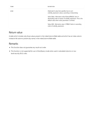
![SUMMARIZE
11/30/2021 • 4 minutes to read
Syntax
SUMMARIZE (<table>, <groupBy_columnName>[, <groupBy_columnName>]…[, <name>, <expression>]…)
Parameters
TERM DEFINITION
table Any DAX expression that returns a table of data.
groupBy_ColumnName (Optional) The qualified name of an existing column used to
create summary groups based on the values found in it. This
parameter cannot be an expression.
name The name given to a total or summarize column, enclosed in
double quotes.
expression Any DAX expression that returns a single scalar value, where
the expression is to be evaluated multiple times (for each
row/context).
Return value
Remarks
Example
Returns a summary table for the requested totals over a set of groups.
A table with the selected columns for the groupBy_columnName arguments and the summarized columns
designed by the name arguments.
Each column for which you define a name must have a corresponding expression; otherwise, an error is
returned. The first argument, name, defines the name of the column in the results. The second argument,
expression, defines the calculation performed to obtain the value for each row in that column.
groupBy_columnName must be either in table or in a related table to table.
Each name must be enclosed in double quotation marks.
The function groups a selected set of rows into a set of summary rows by the values of one or more
groupBy_columnName columns. One row is returned for each group.
This function is not supported for use in DirectQuery mode when used in calculated columns or row-
level security (RLS) rules.
The following example returns a summary of the reseller sales grouped around the calendar year and the
product category name, this result table allows you to do analysis over the reseller sales by year and product](https://image.slidesharecdn.com/funcoesdax-220812141017-bb6cd4dc/85/Funcoes-DAX-pdf-546-320.jpg)
![SUMMARIZE(ResellerSales_USD
, DateTime[CalendarYear]
, ProductCategory[ProductCategoryName]
, "Sales Amount (USD)", SUM(ResellerSales_USD[SalesAmount_USD])
, "Discount Amount (USD)", SUM(ResellerSales_USD[DiscountAmount])
)
DATETIME[CALENDARYEAR
]
PRODUCTCATEGORY[PROD
UCTCATEGORYNAME] [SALES AMOUNT (USD)]
[DISCOUNT AMOUNT
(USD)]
2008 Bikes 12968255.42 36167.6592
2005 Bikes 6958251.043 4231.1621
2006 Bikes 18901351.08 178175.8399
2007 Bikes 24256817.5 276065.992
2008 Components 2008052.706 39.9266
2005 Components 574256.9865 0
2006 Components 3428213.05 948.7674
2007 Components 5195315.216 4226.0444
2008 Clothing 366507.844 4151.1235
2005 Clothing 31851.1628 90.9593
2006 Clothing 455730.9729 4233.039
2007 Clothing 815853.2868 12489.3835
2008 Accessories 153299.924 865.5945
2005 Accessories 18594.4782 4.293
2006 Accessories 86612.7463 1061.4872
2007 Accessories 275794.8403 4756.6546
With ROLLUP
Example
category.
The following table shows a preview of the data as it would be received by any function expecting to receive a
table:
The addition of the ROLLUP syntax modifies the behavior of the SUMMARIZE function by adding rollup rows to
the result on the groupBy_columnName columns. ROLLUP can only be used within a SUMMARIZE expression.
The following example adds rollup rows to the Group-By columns of the SUMMARIZE function call:](https://image.slidesharecdn.com/funcoesdax-220812141017-bb6cd4dc/85/Funcoes-DAX-pdf-547-320.jpg)
![SUMMARIZE(ResellerSales_USD
, ROLLUP( DateTime[CalendarYear], ProductCategory[ProductCategoryName])
, "Sales Amount (USD)", SUM(ResellerSales_USD[SalesAmount_USD])
, "Discount Amount (USD)", SUM(ResellerSales_USD[DiscountAmount])
)
DATETIME[CALENDARYEAR
]
PRODUCTCATEGORY[PROD
UCTCATEGORYNAME] [SALES AMOUNT (USD)]
[DISCOUNT AMOUNT
(USD)]
2008 Bikes 12968255.42 36167.6592
2005 Bikes 6958251.043 4231.1621
2006 Bikes 18901351.08 178175.8399
2007 Bikes 24256817.5 276065.992
2008 Components 2008052.706 39.9266
2005 Components 574256.9865 0
2006 Components 3428213.05 948.7674
2007 Components 5195315.216 4226.0444
2008 Clothing 366507.844 4151.1235
2005 Clothing 31851.1628 90.9593
2006 Clothing 455730.9729 4233.039
2007 Clothing 815853.2868 12489.3835
2008 Accessories 153299.924 865.5945
2005 Accessories 18594.4782 4.293
2006 Accessories 86612.7463 1061.4872
2007 Accessories 275794.8403 4756.6546
2008 15496115.89 41224.3038
2005 7582953.67 4326.4144
2006 22871907.85 184419.1335
2007 30543780.84 297538.0745
76494758.25 527507.9262
Returns the following table,](https://image.slidesharecdn.com/funcoesdax-220812141017-bb6cd4dc/85/Funcoes-DAX-pdf-548-320.jpg)
![With ROLLUPGROUP
Example
SUMMARIZE(ResellerSales_USD
, ROLLUP(ROLLUPGROUP( DateTime[CalendarYear], ProductCategory[ProductCategoryName]))
, "Sales Amount (USD)", SUM(ResellerSales_USD[SalesAmount_USD])
, "Discount Amount (USD)", SUM(ResellerSales_USD[DiscountAmount])
)
DATETIME[CALENDARYEAR
]
PRODUCTCATEGORY[PROD
UCTCATEGORYNAME] [SALES AMOUNT (USD)]
[DISCOUNT AMOUNT
(USD)]
2008 Bikes 12968255.42 36167.6592
2005 Bikes 6958251.043 4231.1621
2006 Bikes 18901351.08 178175.8399
2007 Bikes 24256817.5 276065.992
2008 Components 2008052.706 39.9266
2005 Components 574256.9865 0
2006 Components 3428213.05 948.7674
2007 Components 5195315.216 4226.0444
2008 Clothing 366507.844 4151.1235
2005 Clothing 31851.1628 90.9593
2006 Clothing 455730.9729 4233.039
2007 Clothing 815853.2868 12489.3835
2008 Accessories 153299.924 865.5945
2005 Accessories 18594.4782 4.293
2006 Accessories 86612.7463 1061.4872
2007 Accessories 275794.8403 4756.6546
76494758.25 527507.9262
The addition of ROLLUPGROUP inside a ROLLUP syntax can be used to prevent partial subtotals in rollup rows.
ROLLUPGROUP can only be used within a ROLLUP, ROLLUPADDISSUBTOTAL, or ROLLUPISSUBTOTAL
expression.
The following example shows only the grand total of all years and categories without the subtotal of each year
with all categories:
Returns the following table,](https://image.slidesharecdn.com/funcoesdax-220812141017-bb6cd4dc/85/Funcoes-DAX-pdf-549-320.jpg)
![DATETIME[CALENDARYEAR
]
PRODUCTCATEGORY[PROD
UCTCATEGORYNAME] [SALES AMOUNT (USD)]
[DISCOUNT AMOUNT
(USD)]
With ISSUBTOTAL
Example
SUMMARIZE(ResellerSales_USD
, ROLLUP( DateTime[CalendarYear], ProductCategory[ProductCategoryName])
, "Sales Amount (USD)", SUM(ResellerSales_USD[SalesAmount_USD])
, "Discount Amount (USD)", SUM(ResellerSales_USD[DiscountAmount])
, "Is Sub Total for DateTimeCalendarYear", ISSUBTOTAL(DateTime[CalendarYear])
, "Is Sub Total for ProductCategoryName", ISSUBTOTAL(ProductCategory[ProductCategoryName])
)
[IS SUB TOTAL
FOR
DATETIMECALEN
DARYEAR]
[IS SUB TOTAL
FOR
PRODUCTCATEG
ORYNAME]
DATETIME[CALE
NDARYEAR]
PRODUCTCATEG
ORY[PRODUCTC
ATEGORYNAME]
[SALES AMOUNT
(USD)]
[DISCOUNT
AMOUNT (USD)]
FALSE FALSE
FALSE FALSE 2008 Bikes 12968255.42 36167.6592
FALSE FALSE 2005 Bikes 6958251.043 4231.1621
FALSE FALSE 2006 Bikes 18901351.08 178175.8399
FALSE FALSE 2007 Bikes 24256817.5 276065.992
FALSE FALSE 2008 Components 2008052.706 39.9266
FALSE FALSE 2005 Components 574256.9865 0
FALSE FALSE 2006 Components 3428213.05 948.7674
FALSE FALSE 2007 Components 5195315.216 4226.0444
FALSE FALSE 2008 Clothing 366507.844 4151.1235
FALSE FALSE 2005 Clothing 31851.1628 90.9593
FALSE FALSE 2006 Clothing 455730.9729 4233.039
With ISSUBTOTAL, you can create another column in the SUMMARIZE expression that returns True if the row
contains subtotal values for the column given as argument to ISSUBTOTAL, otherwise returns False. ISSUBTOTAL
can only be used within a SUMMARIZE expression.
The following sample generates an ISSUBTOTAL column for each of the ROLLUP columns in the given
SUMMARIZE function call:
Returns the following table,](https://image.slidesharecdn.com/funcoesdax-220812141017-bb6cd4dc/85/Funcoes-DAX-pdf-550-320.jpg)
![FALSE FALSE 2007 Clothing 815853.2868 12489.3835
FALSE FALSE 2008 Accessories 153299.924 865.5945
FALSE FALSE 2005 Accessories 18594.4782 4.293
FALSE FALSE 2006 Accessories 86612.7463 1061.4872
FALSE FALSE 2007 Accessories 275794.8403 4756.6546
FALSE TRUE
FALSE TRUE 2008 15496115.89 41224.3038
FALSE TRUE 2005 7582953.67 4326.4144
FALSE TRUE 2006 22871907.85 184419.1335
FALSE TRUE 2007 30543780.84 297538.0745
TRUE TRUE 76494758.25 527507.9262
[IS SUB TOTAL
FOR
DATETIMECALEN
DARYEAR]
[IS SUB TOTAL
FOR
PRODUCTCATEG
ORYNAME]
DATETIME[CALE
NDARYEAR]
PRODUCTCATEG
ORY[PRODUCTC
ATEGORYNAME]
[SALES AMOUNT
(USD)]
[DISCOUNT
AMOUNT (USD)]
See also
SUMMARIZECOLUMNS](https://image.slidesharecdn.com/funcoesdax-220812141017-bb6cd4dc/85/Funcoes-DAX-pdf-551-320.jpg)
![SUMMARIZECOLUMNS
11/30/2021 • 5 minutes to read
Syntax
SUMMARIZECOLUMNS( <groupBy_columnName> [, < groupBy_columnName >]…, [<filterTable>]…[, <name>, <expression>]
…)
Parameters
TERM DEFINITION
groupBy_columnName A fully qualified column reference (Table[Column]) to a base
table for which the distinct values are included in the
returned table. Each groupBy_columnName column is cross-
joined (different tables) or auto-existed (same table) with the
subsequent specified columns.
filterTable A table expression which is added to the filter context of all
columns specified as groupBy_columnName arguments. The
values present in the filter table are used to filter before
cross-join/auto-exist is performed.
name A string representing the column name to use for the
subsequent expression specified.
expression Any DAX expression that returns a single value (not a table).
Return value
Remarks
Filter context
Returns a summary table over a set of groups.
A table which includes combinations of values from the supplied columns based on the grouping specified. Only
rows for which at least one of the supplied expressions return a non-blank value are included in the table
returned. If all expressions evaluate to BLANK/NULL for a row, that row is not included in the table returned.
This function does not guarantee any sort order for the results.
A column cannot be specified more than once in the groupBy_columnName parameter. For example, the
following formula is invalid.
SUMMARIZECOLUMNS( Sales[StoreId], Sales[StoreId] )
This function is not supported for use in DirectQuery mode when used in calculated columns or row-
level security (RLS) rules.
Consider the following query:](https://image.slidesharecdn.com/funcoesdax-220812141017-bb6cd4dc/85/Funcoes-DAX-pdf-552-320.jpg)
![SUMMARIZECOLUMNS (
'Sales Territory'[Category],
FILTER('Customer', 'Customer' [First Name] = "Alicia")
)
SUMMARIZECOLUMNS (
'Sales Territory'[Category], 'Customer' [Education],
FILTER('Customer', 'Customer'[First Name] = "Alicia")
)
With IGNORE
Example
SUMMARIZECOLUMNS(
Sales[CustomerId], "Total Qty",
IGNORE( SUM( Sales[Qty] ) ),
"BlankIfTotalQtyIsNot3", IF( SUM( Sales[Qty] )=3, 3 )
)
CUSTOMERID TOTALQTY BLANKIFTOTALQTYISNOT3
A 5
B 3 3
C 3 3
CUSTOMERID TOTALQTY BLANKIFTOTALQTYISNOT3
B 3 3
C 3 3
In this query, without a measure the groupBy columns do not contain any columns from the FILTER expression
(for example, from Customer table). The filter is not applied to the groupBy columns. The Sales Territory and
Customer tables may be indirectly related through the Reseller sales fact table. Since they're not directly related,
the filter expression is a no-op and the groupBy columns are not impacted.
However, with this query:
The groupBy columns contain a column which is impacted by the filter and that filter is applied to the groupBy
results.
The IGNORE syntax can be used to modify the behavior of the SUMMARIZECOLUMNS function by omitting
specific expressions from the BLANK/NULL evaluation. Rows for which all expressions not using IGNORE return
BLANK/NULL will be excluded independent of whether the expressions which do use IGNORE evaluate to
BLANK/NULL or not. IGNORE can only be used within a SUMMARIZECOLUMNS expression.
This rolls up the Sales[CustomerId] column, creating a subtotal for all customers in the given grouping. Without
IGNORE, the result is:
With IGNORE,
All expression ignored,](https://image.slidesharecdn.com/funcoesdax-220812141017-bb6cd4dc/85/Funcoes-DAX-pdf-553-320.jpg)
![SUMMARIZECOLUMNS(
Sales[CustomerId], "Blank",
IGNORE( Blank() ), "BlankIfTotalQtyIsNot5",
IGNORE( IF( SUM( Sales[Qty] )=5, 5 ) )
)
CUSTOMERID TOTALQTY BLANKIFTOTALQTYISNOT3
A 5
B
C
With NONVISUAL
Example
DEFINE
MEASURE FactInternetSales[Sales] = SUM(FactInternetSales[Sales Amount])
EVALUATE
SUMMARIZECOLUMNS
(
DimDate[CalendarYear],
NONVISUAL(TREATAS({2007, 2008}, DimDate[CalendarYear])),
"Sales", [Sales],
"Visual Total Sales", CALCULATE([Sales], ALLSELECTED(DimDate[CalendarYear]))
)
ORDER BY [CalendarYear]
DIMDATE[CALENDARYEAR] [SALES] [VISUAL TOTAL SALES]
2007 9,791,060.30 29,358,677.22
2008 9,770,899.74 29,358,677.22
Even though both expressions return blank for some rows, they're included since there are no unignored
expressions which return blank.
The NONVISUAL function marks a value filter in SUMMARIZECOLUMNS function as not affecting measure
values, but only applying to groupBy columns. NONVISUAL can only be used within a SUMMARIZECOLUMNS
expression.
Returns the result where [Visual Total Sales] is the total across all years:
In contrast, the same query without the NONVISUAL function:](https://image.slidesharecdn.com/funcoesdax-220812141017-bb6cd4dc/85/Funcoes-DAX-pdf-554-320.jpg)
![DEFINE
MEASURE FactInternetSales[Sales] = SUM(FactInternetSales[Sales Amount])
EVALUATE
SUMMARIZECOLUMNS
(
DimDate[CalendarYear],
TREATAS({2007, 2008}, DimDate[CalendarYear]),
"Sales", [Sales],
"Visual Total Sales", CALCULATE([Sales], ALLSELECTED(DimDate[CalendarYear]))
)
ORDER BY [CalendarYear]
DIMDATE[CALENDARYEAR] [SALES] [VISUAL TOTAL SALES]
2007 9,791,060.30 19,561,960.04
2008 9,770,899.74 19,561,960.04
With ROLLUPADDISSUBTOTAL
Example with single subtotal
DEFINE
VAR vCategoryFilter =
TREATAS({"Accessories", "Clothing"}, Product[Category])
VAR vSubcategoryFilter =
TREATAS({"Bike Racks", "Mountain Bikes"}, Product[Subcategory])
EVALUATE
SUMMARIZECOLUMNS
(
ROLLUPADDISSUBTOTAL
(
Product[Category], "IsCategorySubtotal", vCategoryFilter,
Product[Subcategory], "IsSubcategorySubtotal", vSubcategoryFilter
),
"Total Qty", SUM(Sales[Qty])
)
ORDER BY
[IsCategorySubtotal] DESC, [Category],
[IsSubcategorySubtotal] DESC, [Subcategory]
CATEGORY SUBCATEGORY
ISCATEGORYSUBTOT
AL
ISSUBCATEGORYSUB
TOTAL TOTAL QTY
True True 60398
Accessories False True 36092
Accessories Bike Racks False False 328
Returns the result where [Visual Total Sales] is the total across the two selected years:
The addition of the ROLLUPADDISSUBTOTAL syntax modifies the behavior of the SUMMARIZECOLUMNS
function by adding rollup/subtotal rows to the result based on the groupBy_columnName columns.
ROLLUPADDISSUBTOTAL can only be used within a SUMMARIZECOLUMNS expression.
Returns the following table,](https://image.slidesharecdn.com/funcoesdax-220812141017-bb6cd4dc/85/Funcoes-DAX-pdf-555-320.jpg)
![Bikes Mountain Bikes False False 4970
Clothing False True 9101
CATEGORY SUBCATEGORY
ISCATEGORYSUBTOT
AL
ISSUBCATEGORYSUB
TOTAL TOTAL QTY
Example with multiple subtotals
SUMMARIZECOUMNS (
Regions[State], ROLLUPADDISSUBTOTAL ( Sales[CustomerId], "IsCustomerSubtotal" ),
ROLLUPADDISSUBTOTAL ( Sales[Date], "IsDateSubtotal"), "Total Qty", SUM( Sales[Qty] )
)
CUSTOMERID
ISCUSTOMERSUB
TOTAL STATE TOTAL QTY DATE ISDATESUBTOTAL
A FALSE WA 5 7/10/2014
B FALSE WA 1 7/10/2014
B FALSE WA 2 7/11/2014
C FALSE OR 2 7/10/2014
C FALSE OR 1 7/11/2014
TRUE WA 6 7/10/2014
TRUE WA 2 7/11/2014
TRUE OR 2 7/10/2014
TRUE OR 1 7/11/2014
A FALSE WA 5 TRUE
B FALSE WA 3 TRUE
C FALSE OR 3 TRUE
TRUE WA 8 TRUE
TRUE OR 3 TRUE
With ROLLUPGROUP
Sales is grouped by state, by customer, by date, with subtotals for 1. Sales by state, by date 2. Sales by State, by
Customer 3. Rolled up on both customer and date leading to sales by state.
Returns the following table,
Like with the SUMMARIZE function, ROLLUPGROUP can be used together with ROLLUPADDISSUBTOTAL to
specify which summary groups/granularities (subtotals) to include, reducing the number of subtotal rows](https://image.slidesharecdn.com/funcoesdax-220812141017-bb6cd4dc/85/Funcoes-DAX-pdf-556-320.jpg)
![Example with multiple subtotals
SUMMARIZECOLUMNS(
ROLLUPADDISSUBTOTAL( Sales[CustomerId], "IsCustomerSubtotal" ),
ROLLUPADDISSUBTOTAL(ROLLUPGROUP(Regions[City], Regions[State]), "IsCityStateSubtotal"),"Total Qty", SUM(
Sales[Qty] )
)
STATE CUSTOMERID
ISCUSTOMERSUB
TOTAL TOTAL QTY CITY
ISCITYSTATESUB
TOTAL
WA A FALSE 2 Bellevue FALSE
WA B FALSE 2 Bellevue FALSE
WA A FALSE 3 Redmond FALSE
WA B FALSE 1 Redmond FALSE
OR C FALSE 3 Portland FALSE
WA TRUE 4 Bellevue FALSE
WA TRUE 4 Redmond FALSE
OR TRUE 3 Portland FALSE
A FALSE 5 FALSE
B FALSE 3 TRUE
C FALSE 3 TRUE
TRUE 11 TRUE
See also
returned. ROLLUPGROUP can only be used within a SUMMARIZECOLUMNS or SUMMARIZE expression.
Still grouped by City and State, but rolled together when reporting a subtotal returns the following table,
SUMMARIZE](https://image.slidesharecdn.com/funcoesdax-220812141017-bb6cd4dc/85/Funcoes-DAX-pdf-557-320.jpg)
![Table constructor
11/30/2021 • 2 minutes to read
Syntax
{ <scalarExpr1>, <scalarExpr2>, … }
{ ( <scalarExpr1>, <scalarExpr2>, … ), ( <scalarExpr1>, <scalarExpr2>, … ), … }
Parameters
TERM DEFINITION
scalarExprN Any DAX expression that returns a scalar value.
Return value
Remarks
Example 1
EVALUATE { 1, 2, 3 }
EVALUATE { (1), (2), (3) }
[VALUE]
1
2
Returns a table of one or more columns.
A table of one or more columns. When there is only one column, the name of the column is Value. When there
are N columns where N > 1, the names of the columns from left to right are Value1, Value2, …, ValueN.
The first syntax returns a table of a single column. The second syntax returns a table of one or more
columns.
The number of scalar expressions must be the same for all rows.
When the data types of the values for a column are different in different rows, all values are converted to
a common data type.
The following DAX queries:
and
Return the following table of a single column:](https://image.slidesharecdn.com/funcoesdax-220812141017-bb6cd4dc/85/Funcoes-DAX-pdf-558-320.jpg)
![3
[VALUE]
Example 2
EVALUATE
{
(1.5, DATE(2017, 1, 1), CURRENCY(199.99), "A"),
(2.5, DATE(2017, 1, 2), CURRENCY(249.99), "B"),
(3.5, DATE(2017, 1, 3), CURRENCY(299.99), "C")
}
[VALUE1] [VALUE2] [VALUE3] [VALUE4]
1.5 1/1/2017 199.99 A
2.5 1/2/2017 249.99 B
3.5 1/3/2017 299.99 C
Example 3
EVALUATE { 1, DATE(2017, 1, 1), TRUE, "A" }
[VALUE]
1
1/1/2017
TRUE
A
The following DAX query:
Returns,
The following DAX query:
Returns the following table of a single column of String data type:](https://image.slidesharecdn.com/funcoesdax-220812141017-bb6cd4dc/85/Funcoes-DAX-pdf-559-320.jpg)
![TOPN
11/30/2021 • 2 minutes to read
Syntax
TOPN(<n_value>, <table>, <orderBy_expression>, [<order>[, <orderBy_expression>, [<order>]]…])
Parameters
VALUE ALTERNATE VALUE DESCRIPTION
0 (zero) FALSE Sorts in descending order of values of
order_by.
This is the default value when order
parameter is omitted.
1 TRUE Ranks in ascending order of order_by.
Return value
Remarks
Returns the top N rows of the specified table.
The number of rows to return. It is any DAX expression that returns a single scalar value, where the expression is
to be evaluated multiple times (for each row/context).
See the remarks section to understand when the number of rows returned could possible be larger than
n_value.
See the remarks section to understand when an empty table is returned.
table Any DAX expression that returns a table of data from where to extract the top 'n' rows.
orderBy_expression
Any DAX expression where the result value is used to sort the table and it is evaluated for each row of table.
order (Optional) A value that specifies how to sort orderBy_expression values, ascending or descending:
A table with the top N rows of table or an empty table if n_value is 0 (zero) or less. Rows are not necessarily
sorted in any particular order.
If there is a tie, in order_by values, at the N-th row of the table, then all tied rows are returned. Then, when
there are ties at the N-th row the function might return more than n rows.
If n_value is 0 (zero) or less then TOPN returns an empty table.
TOPN does not guarantee any sort order for the results.
This function is not supported for use in DirectQuery mode when used in calculated columns or row-
level security (RLS) rules.](https://image.slidesharecdn.com/funcoesdax-220812141017-bb6cd4dc/85/Funcoes-DAX-pdf-560-320.jpg)
![Example
= SUMX(TOPN(10, SUMMARIZE(Product, [ProductKey], "TotalSales",
SUMX(RELATED(InternetSales_USD[SalesAmount_USD]), InternetSales_USD[SalesAmount_USD]) +
SUMX(RELATED(ResellerSales_USD[SalesAmount_USD]), ResellerSales_USD[SalesAmount_USD]))
The following sample creates a measure with the sales of the top 10 sold products.](https://image.slidesharecdn.com/funcoesdax-220812141017-bb6cd4dc/85/Funcoes-DAX-pdf-561-320.jpg)
![TREATAS
11/30/2021 • 2 minutes to read
Syntax
TREATAS(table_expression, <column>[, <column>[, <column>[,…]]]} )
Parameters
TERM DEFINITION
table_expression An expression that results in a table.
column One or more existing columns. It cannot be an expression.
Return value
Remarks
Example
CALCULATE(
SUM(Sales[Amount]),
TREATAS(VALUES(DimProduct1[ProductCategory]), DimProduct2[ProductCategory])
)
See also
Applies the result of a table expression as filters to columns from an unrelated table.
A table that contains all the rows in column(s) that are also in table_expression.
The number of columns specified must match the number of columns in the table expression and be in
the same order.
If a value returned in the table expression does not exist in the column, it is ignored. For example,
TREATAS({"Red", "Green", "Yellow"}, DimProduct[Color]) sets a filter on column DimProduct[Color] with
three values "Red", "Green", and "Yellow". If "Yellow" does not exist in DimProduct[Color], the effective
filter values would are "Red" and "Green".
Best for use when a relationship does not exist between the tables. If you have multiple relationships
between the tables involved, consider using USERELATIONSHIP instead.
This function is not supported for use in DirectQuery mode when used in calculated columns or row-
level security (RLS) rules.
In the following example, the model contains two unrelated product tables. If a user applies a filter to
DimProduct1[ProductCategory] selecting Bikes, Seats, Tires, the same filter, Bikes, Seats, Tires is applied to
DimProduct2[ProductCategory].](https://image.slidesharecdn.com/funcoesdax-220812141017-bb6cd4dc/85/Funcoes-DAX-pdf-562-320.jpg)

![UNION
11/30/2021 • 2 minutes to read
Syntax
UNION(<table_expression1>, <table_expression2> [,<table_expression>]…)
Parameters
TERM DEFINITION
table_expression Any DAX expression that returns a table.
Return value
Remarks
Example
UNION(UsaInventory, IndInventory)
Creates a union (join) table from a pair of tables.
A table that contains all the rows from each of the two table expressions.
The two tables must have the same number of columns.
Columns are combined by position in their respective tables.
The column names in the return table will match the column names in table_expression1.
Duplicate rows are retained.
The returned table has lineage where possible. For example, if the first column of each table_expression
has lineage to the same base column C1 in the model, the first column in the UNION result will have
lineage to C1. However, if combined columns have lineage to different base columns, or if there is an
extension column, the resulting column in UNION will have no lineage.
When data types differ, the resulting data type is determined based on the rules for data type coercion.
The returned table will not contain columns from related tables.
This function is not supported for use in DirectQuery mode when used in calculated columns or row-
level security (RLS) rules.
The following expression creates a union by combining the USAInventory table and the INDInventory table into
a single table:
USAInventory](https://image.slidesharecdn.com/funcoesdax-220812141017-bb6cd4dc/85/Funcoes-DAX-pdf-564-320.jpg)
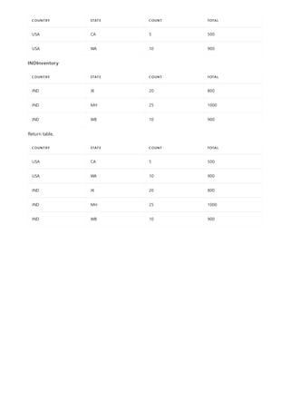
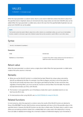
![NOTE
MYORDERS TABLE MYSALES TABLE
June 1 June 1 sales
June 2 June 2 sales
(no order dates have been entered) June 3 sales
Example
= COUNTROWS(VALUES('InternetSales_USD'[SalesOrderNumber]))
ROW LABELS COUNT INVOICES
Accessories 18,208
Bikes 15,205
Clothing 7,461
Grand Total 27,659
See also
data can occur when one table is being updated and the related table is not.
When the argument is a table name, the result of the VALUES function returns all rows in the specified table plus
a blank row, if there is a violation of referential integrity. The DISTINCT function removes duplicate rows and
returns unique rows in the specified table.
The DISTINCT function allows a column name or any valid table expression to be its argument but the VALUES function
only accepts a column name or a table name as the argument.
The following table summarizes the mismatch between data that can occur in two related tables when
referential integrity is not preserved.
If you use the DISTINCT function to return a list of dates, only two dates would be returned. However, if you use
the VALUES function, the function returns the two dates plus an additional blank member. Also, any row from
the MySales table that does not have a matching date in the MyOrders table will be "matched" to this unknown
member.
The following formula counts the number of unique invoices (sales orders), and produces the following results
when used in a report that includes the Product Category Names:
Returns
FILTER function
COUNTROWS function
Filter functions](https://image.slidesharecdn.com/funcoesdax-220812141017-bb6cd4dc/85/Funcoes-DAX-pdf-567-320.jpg)
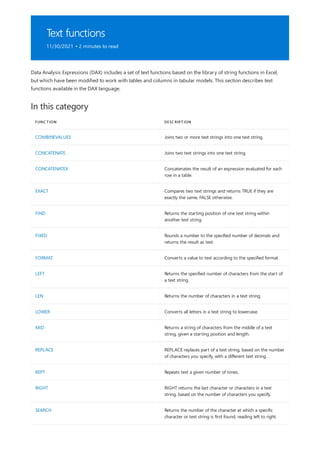
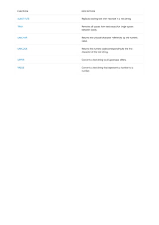
![COMBINEVALUES
11/30/2021 • 2 minutes to read
Syntax
COMBINEVALUES(<delimiter>, <expression>, <expression>[, <expression>]…)
Parameters
TERM DEFINITION
delimiter A separator to use during concatenation. Must be a
constant value.
expression A DAX expression whose value will be be joined into a single
text string.
Return value
Remarks
Joins two or more text strings into one text string. The primary purpose of this function is to support multi-
column relationships in DirectQuery models. See Remarks for details.
The concatenated string.
The COMBINEVALUES function assumes, but does not validate, that when the input values are different,
the output strings are also different. Based on this assumption, when COMBINEVALUES is used to create
calculated columns in order to build a relationship that joins multiple columns from two DirectQuery
tables, an optimized join condition is generated at query time. For example, if users want to create a
relationship between Table1(Column1, Column2) and Table2(Column1, Column2), they can create two
calculated columns, one on each table, as:
Table1[CalcColumn] = COMBINEVALUES(",", Table1[Column1], Table1[Column2])
and
Table2[CalcColumn] = COMBINEVALUES(",", Table2[Column1], Table2[Column2]) ,
And then create a relationship between Table1[CalcColumn] and Table2[CalcColumn] . Unlike other DAX
functions and operators, which are translated literally to the corresponding SQL operators and functions,
the above relationship generates a SQL join predicate as:
(Table1.Column1 = Table2.Column1 OR Table1.Column1 IS NULL AND Table2.Column1 IS NULL)
and
(Table1.Column2 = Table2.Column2 OR Table1.Column2 IS NULL AND Table2.Column2 IS NULL) .
The join predicate can potentially deliver much better query performance than one that involves complex
SQL operators and functions.](https://image.slidesharecdn.com/funcoesdax-220812141017-bb6cd4dc/85/Funcoes-DAX-pdf-570-320.jpg)
![Example
[MONTH]
January,2007
February,2007
March,2007
April,2007
May,2007
June,2007
July,2007
August,2007
September,2007
October,2007
November,2007
December,2007
January,2008
January,2008
February,2008
March,2008
April,2008
The COMBINEVALUES function relies on users to choose the appropriate delimiter to ensure that unique
combinations of input values produce distinct output strings but it does not validate that the assumption
is true. For example, if users choose "| " as the delimiter, but one row in Table1 has
Table1[Column1] = "| " and Table2 [Column2] = " " , while one row in Table2 has Table2[Column1] = " "
and Table2[Column2] = "| " , the two concatenated outputs will be the same "|| " , which seem to
indicate that the two rows are a match in the join operation. The two rows are not joined together if both
tables are from the same DirectQuery source although they are joined together if both tables are
imported.
The following DAX query:
EVALUATE DISTINCT(SELECTCOLUMNS(DimDate, "Month", COMBINEVALUES(",", [MonthName], [CalendarYear])))
Returns the following single column table:](https://image.slidesharecdn.com/funcoesdax-220812141017-bb6cd4dc/85/Funcoes-DAX-pdf-571-320.jpg)
![May,2008
June,2008
July,2008
August,2008
September,2008
October,2008
November,2008
December,2008
[MONTH]](https://image.slidesharecdn.com/funcoesdax-220812141017-bb6cd4dc/85/Funcoes-DAX-pdf-572-320.jpg)

![= CONCATENATE(Customer[LastName], CONCATENATE(", ", Customer[FirstName]))
Example: Conditional Concatenation of Strings in Columns
= CONCATENATE( [FirstName]&" ", CONCATENATE( IF( LEN([MiddleName])>1, LEFT([MiddleName],1)&" ", ""),
[LastName]))
Example: Concatenation of Columns with Different Data Types
PRODUCT DESCRIPTION
PRODUCT ABBREVIATION
(COLUMN 1 OF
COMPOSITE KEY)
PRODUCT NUMBER
(COLUMN 2 OF
COMPOSITE KEY)
NEW GENERATED KEY
COLUMN
Mountain bike MTN 40 MTN40
Mountain bike MTN 42 MTN42
= CONCATENATE('Products'[Product abbreviation],'Products'[Product number])
= [Product abbreviation] & "-" & [Product number]
See also
values that you want to use as arguments.
The sample formula creates a new calculated column in the Customer table with the full customer name as a
combination of first name, middle initial, and last name. If there is no middle name, the last name comes directly
after the first name. If there is a middle name, only the first letter of the middle name is used and the initial letter
is followed by a period.
This formula uses nested CONCATENATE and IF functions, together with the ampersand (&) operator, to
conditionally concatenate three string values and add spaces as separators.
The following example demonstrates how to concatenate values in columns that have different data types. If the
value that you are concatenating is numeric, the value will be implicitly converted to text. If both values are
numeric, both values will be cast to text and concatenated as if they were strings.
The CONCATENATE function in DAX accepts only two arguments, whereas the Excel CONCATENATE function
accepts up to 255 arguments. If you need to add more arguments, you can use the ampersand (&) operator. For
example, the following formula produces the results, MTN-40 and MTN-42.
Text functions](https://image.slidesharecdn.com/funcoesdax-220812141017-bb6cd4dc/85/Funcoes-DAX-pdf-574-320.jpg)
![CONCATENATEX
11/30/2021 • 2 minutes to read
Syntax
CONCATENATEX(<table>, <expression>[, <delimiter> [, <orderBy_expression> [, <order>]]...])
Parameters
TERM DEFINITION
table The table containing the rows for which the expression will
be evaluated.
expression The expression to be evaluated for each row of table.
delimiter (Optional) A separator to use during concatenation.
orderBy_expression (Optional) Any DAX expression where the result value is
used to sort the concatenated values in the output string. It
is evaluated for each row of table.
order (Optional) A value that specifies how to sort
orderBy_expression values, ascending or descending.
VALUE ALTERNATE VALUES DESCRIPTION
0 (zero) FALSE, DESC Sorts in descending order of values of
orderBy_expression.
This is the default value when the
order parameter is omitted.
1 TRUE, ASC Sorts in ascending order of values of
orderBy_expression.
Return value
Remarks
Concatenates the result of an expression evaluated for each row in a table.
The order parameter accepts the following values:
A text string.
This function takes as its first argument a table or an expression that returns a table. The second
argument is a column that contains the values you want to concatenate, or an expression that returns a
value.
Concatenated values are not necessarily sorted in any particular order, unless orderBy_expression is](https://image.slidesharecdn.com/funcoesdax-220812141017-bb6cd4dc/85/Funcoes-DAX-pdf-575-320.jpg)
![Example
FIRSTNAME LASTNAME
Alan Brewer
Michael Blythe
CONCATENATEX(Employees, [FirstName] & " " & [LastName], ",")
specified.
This function is not supported for use in DirectQuery mode when used in calculated columns or row-
level security (RLS) rules.
Employees table
The following formula:
Returns:
"Alan Brewer, Michael Blythe"](https://image.slidesharecdn.com/funcoesdax-220812141017-bb6cd4dc/85/Funcoes-DAX-pdf-576-320.jpg)
![EXACT
11/30/2021 • 2 minutes to read
Syntax
EXACT(<text1>,<text2>)
Parameters
TERM DEFINITION
text1 The first text string or column that contains text.
text2 The second text string or column that contains text.
Return value
Example
= EXACT([Column1],[Column2])
See also
Compares two text strings and returns TRUE if they are exactly the same, FALSE otherwise. EXACT is case-
sensitive but ignores formatting differences. You can use EXACT to test text being entered into a document.
True or false. (Boolean)
The following formula checks the value of Column1 for the current row against the value of Column2 for the
current row, and returns TRUE if they are the same, and returns FALSE if they are different.
Text functions](https://image.slidesharecdn.com/funcoesdax-220812141017-bb6cd4dc/85/Funcoes-DAX-pdf-577-320.jpg)
![FIND
11/30/2021 • 2 minutes to read
Syntax
FIND(<find_text>, <within_text>[, [<start_num>][, <NotFoundValue>]])
Parameters
TERM DEFINITION
find_text The text you want to find. Use double quotes (empty text) to
match the first character in within_text.
within_text The text containing the text you want to find.
start_num (optional) The character at which to start the search; if
omitted, start_num = 1. The first character in within_text
is character number 1.
NotFoundValue (optional) The value that should be returned when the
operation does not find a matching substring, typically 0, -1,
or BLANK().
Return value
Remarks
Example
= FIND("BMX","line of BMX racing goods")
Returns the starting position of one text string within another text string. FIND is case-sensitive.
Number that shows the starting point of the text string you want to find.
Whereas Microsoft Excel has multiple versions of the FIND function to accommodate single-byte
character set (SBCS) and double-byte character set (DBCS) languages, DAX uses Unicode and counts each
character the same way; therefore, you do not need to use a different version depending on the character
type.
This function is not supported for use in DirectQuery mode when used in calculated columns or row-
level security (RLS) rules.
FIND does not support wildcards. To use wildcards, use SEARCH.
The following formula finds the position of the first letter of the product designation, BMX, in the string that
contains the product description.](https://image.slidesharecdn.com/funcoesdax-220812141017-bb6cd4dc/85/Funcoes-DAX-pdf-578-320.jpg)

![FIXED
11/30/2021 • 2 minutes to read
Syntax
FIXED(<number>, <decimals>, <no_commas>)
Parameters
TERM DEFINITION
number The number you want to round and convert to text, or a
column containing a number.
decimals (optional) The number of digits to the right of the decimal
point; if omitted, 2.
no_commas (optional) A logical value: if 1, do not display commas in the
returned text; if 0 or omitted, display commas in the
returned text.
Return value
Remarks
Example
= FIXED([PctCost],3,1)
Rounds a number to the specified number of decimals and returns the result as text. You can specify that the
result be returned with or without commas.
A number represented as text.
If the value used for the decimals parameter is negative, number is rounded to the left of the decimal
point.
If you omit decimals, it is assumed to be 2.
If no_commas is 0 or is omitted, then the returned text includes commas as usual.
The major difference between formatting a cell containing a number by using a command and formatting
a number directly with the FIXED function is that FIXED converts its result to text. A number formatted
with a command from the formatting menu is still a number.
This function is not supported for use in DirectQuery mode when used in calculated columns or row-
level security (RLS) rules.
The following example gets the numeric value for the current row in column, PctCost, and returns it as text with
4 decimal places and no commas.](https://image.slidesharecdn.com/funcoesdax-220812141017-bb6cd4dc/85/Funcoes-DAX-pdf-580-320.jpg)

![FORMAT
11/30/2021 • 13 minutes to read
Syntax
FORMAT(<value>, <format_string>[, <locale_name>])
Parameters
TERM DEFINITION
value A value or expression that evaluates to a single value.
format_string A string with the formatting template.
locale_name (Optional) Name of the locale to be used by the function.
Possible values are strings accepted by the Windows API
function LocaleNameToLCID().
Return value
NOTE
Remarks
Converts a value to text according to the specified format.
A string containing value formatted as defined by format_string.
If value is BLANK, the function returns an empty string.
If format_string is BLANK, the value is formatted with a "General Number" or "General Date" format (according to value
data type).
Predefined format strings use the model culture property when formatting the result. By default, the
model culture property is set according to the user locale of the computer. For new Power BI Desktop
models, the model culture property can be changed in Options > Regional Settings > Model language.
For Analysis Services, model culture is set according to the Language property initially defined by the
instance.
The format strings supported as an argument to the DAX FORMAT function are based on the format
strings used by Visual Basic (OLE Automation), not on the format strings used by the .NET Framework.
Therefore, you might get unexpected results or an error if the argument doesn't match any defined
format strings. For example, "p" as an abbreviation for "Percent" isn't supported. Strings that you provide
as an argument to the FORMAT function that aren't included in the list of predefined format strings are
handled as part of a custom format string, or as a string literal.
This function is not supported for use in DirectQuery mode when used in calculated columns or row-
level security (RLS) rules.](https://image.slidesharecdn.com/funcoesdax-220812141017-bb6cd4dc/85/Funcoes-DAX-pdf-582-320.jpg)
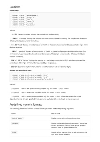
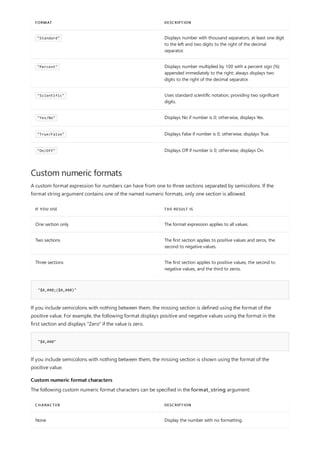
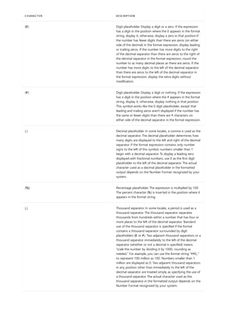
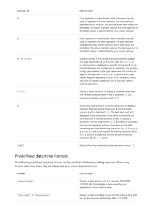
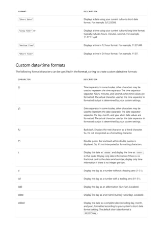
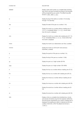
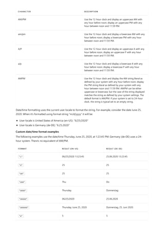
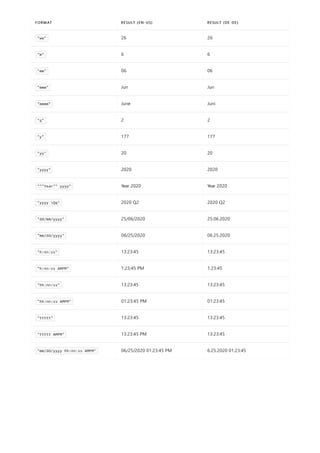
![LEFT
11/30/2021 • 2 minutes to read
Syntax
LEFT(<text>, <num_chars>)
Parameters
TERM DEFINITION
text The text string containing the characters you want to extract,
or a reference to a column that contains text.
num_chars (optional) The number of characters you want LEFT to
extract; if omitted, 1.
Return value
Remarks
Example
= CONCATENATE(LEFT('Reseller'[ResellerName],LEFT(GeographyKey,3))
See also
Returns the specified number of characters from the start of a text string.
A text string.
Whereas Microsoft Excel contains different functions for working with text in single-byte and double-byte
character languages, DAX works with Unicode and stores all characters as the same length; therefore, a
single function is enough.
This function is not supported for use in DirectQuery mode when used in calculated columns or row-
level security (RLS) rules.
The following example returns the first five characters of the company name in the column [ResellerName] and
the first five letters of the geographical code in the column [GeographyKey] and concatenates them, to create an
identifier.
If the num_chars argument is a number that is larger than the number of characters available, the function
returns the maximum characters available and does not raise an error. For example, the column [GeographyKey]
contains numbers such as 1, 12 and 311; therefore the result also has variable length.
Text functions](https://image.slidesharecdn.com/funcoesdax-220812141017-bb6cd4dc/85/Funcoes-DAX-pdf-591-320.jpg)
![LEN
11/30/2021 • 2 minutes to read
Syntax
LEN(<text>)
Parameters
TERM DEFINITION
text The text whose length you want to find, or a column that
contains text. Spaces count as characters.
Return value
Remarks
Example
= LEN([AddressLine1])+LEN([AddressLin2])
Returns the number of characters in a text string.
A whole number indicating the number of characters in the text string.
Whereas Microsoft Excel has different functions for working with single-byte and double-byte character
languages, DAX uses Unicode and stores all characters with the same length.
LEN always counts each character as 1, no matter what the default language setting is.
If you use LEN with a column that contains non-text values, such as dates or Booleans, the function
implicitly casts the value to text, using the current column format.
The following formula sums the lengths of addresses in the columns, [AddressLine1] and [AddressLine2].](https://image.slidesharecdn.com/funcoesdax-220812141017-bb6cd4dc/85/Funcoes-DAX-pdf-592-320.jpg)
![LOWER
11/30/2021 • 2 minutes to read
Syntax
LOWER(<text>)
Parameters
TERM DEFINITION
text The text you want to convert to lowercase, or a reference to
a column that contains text.
Return value
Remarks
Example
= LOWER('New Products'[ProductCode])
See also
Converts all letters in a text string to lowercase.
Text in lowercase.
Characters that are not letters are not changed. For example, the formula = LOWER("123ABC") returns 123abc.
The following formula gets each row in the column, [ProductCode], and converts the value to all lowercase.
Numbers in the column are not affected.
Text functions](https://image.slidesharecdn.com/funcoesdax-220812141017-bb6cd4dc/85/Funcoes-DAX-pdf-593-320.jpg)
![MID
11/30/2021 • 2 minutes to read
Syntax
MID(<text>, <start_num>, <num_chars>)
Parameters
TERM DEFINITION
text The text string from which you want to extract the
characters, or a column that contains text.
start_num The position of the first character you want to extract.
Positions start at 1.
num_chars The number of characters to return.
Return value
Remarks
Examples
MID("abcde",2,3))
MID('Reseller'[ResellerName],1,5))
See also
Returns a string of characters from the middle of a text string, given a starting position and length.
A string of text of the specified length.
Whereas Microsoft Excel has different functions for working with single-byte and double-byte characters
languages, DAX uses Unicode and stores all characters with the same length.
The following expression,
Returns "bcd".
The following expression,
Returns the same result as LEFT([ResellerName],5) . Both expressions return the first 5 letters of column,
[ResellerName] .
Text functions](https://image.slidesharecdn.com/funcoesdax-220812141017-bb6cd4dc/85/Funcoes-DAX-pdf-594-320.jpg)
![REPLACE
11/30/2021 • 2 minutes to read
Syntax
REPLACE(<old_text>, <start_num>, <num_chars>, <new_text>)
Parameters
TERM DEFINITION
old_text The string of text that contains the characters you want to
replace, or a reference to a column that contains text.
start_num The position of the character in old_text that you want to
replace with new_text.
num_chars The number of characters that you want to replace.
Warning: If the argument, num_chars, is a blank or
references a column that evaluates to a blank, the string for
new_text is inserted at the position, start_num, without
replacing any characters. This is the same behavior as in
Excel.
new_text The replacement text for the specified characters in
old_text.
Return value
Remarks
Example
= REPLACE('New Products'[Product Code],1,2,"OB")
REPLACE replaces part of a text string, based on the number of characters you specify, with a different text
string.
A text string.
Whereas Microsoft Excel has different functions for use with single-byte and double-byte character
languages, DAX uses Unicode and therefore stores all characters as the same length.
This function is not supported for use in DirectQuery mode when used in calculated columns or row-
level security (RLS) rules.
The following formula creates a new calculated column that replaces the first two characters of the product code
in column, [ProductCode], with a new two-letter code, OB.](https://image.slidesharecdn.com/funcoesdax-220812141017-bb6cd4dc/85/Funcoes-DAX-pdf-595-320.jpg)

![REPT
11/30/2021 • 2 minutes to read
Syntax
REPT(<text>, <num_times>)
Parameters
TERM DEFINITION
text The text you want to repeat.
num_times A positive number specifying the number of times to repeat
text.
Return value
Remarks
Example: Repeating Literal Strings
= REPT("85",3)
Example: Repeating Column Values
= REPT([MyText],[MyNumber])
MYTEXT MYNUMBER CALCULATEDCOLUMN1
Text 2 TextText
Repeats text a given number of times. Use REPT to fill a cell with a number of instances of a text string.
A string containing the changes.
If number_times is 0 (zero), REPT returns a blank.
If number_times is not an integer, it is truncated.
The result of the REPT function cannot be longer than 32,767 characters, or REPT returns an error.
The following example returns the string, 85, repeated three times.
The following example returns the string in the column, [MyText], repeated for the number of times in the
column, [MyNumber]. Because the formula extends for the entire column, the resulting string depends on the
text and number value in each row.](https://image.slidesharecdn.com/funcoesdax-220812141017-bb6cd4dc/85/Funcoes-DAX-pdf-597-320.jpg)
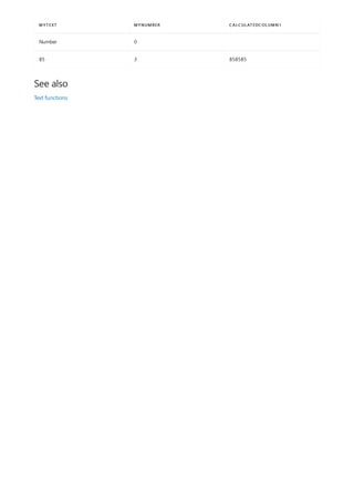
![RIGHT
11/30/2021 • 2 minutes to read
Syntax
RIGHT(<text>, <num_chars>)
Parameters
TERM DEFINITION
text The text string that contains the characters you want to
extract, or a reference to a column that contains text.
num_chars (optional) The number of characters you want RIGHT to
extract; is omitted, 1. You can also use a reference to a
column that contains numbers.
Return value
Remarks
Example: Returning a Fixed Number of Characters
= RIGHT('New Products'[ProductCode],2)
Example: Using a Column Reference to Specify Character Count
= RIGHT('New Products'[ProductCode],[MyCount])
RIGHT returns the last character or characters in a text string, based on the number of characters you specify.
If the column reference does not contain text, it is implicitly cast as text.
A text string containing the specified right-most characters.
RIGHT always counts each character, whether single-byte or double-byte, as 1, no matter what the default
language setting is.
This function is not supported for use in DirectQuery mode when used in calculated columns or row-
level security (RLS) rules.
The following formula returns the last two digits of the product code in the New Products table.
The following formula returns a variable number of digits from the product code in the New Products table,
depending on the number in the column, MyCount. If there is no value in the column, MyCount, or the value is a
blank, RIGHT also returns a blank.](https://image.slidesharecdn.com/funcoesdax-220812141017-bb6cd4dc/85/Funcoes-DAX-pdf-599-320.jpg)

![SEARCH
11/30/2021 • 2 minutes to read
Syntax
SEARCH(<find_text>, <within_text>[, [<start_num>][, <NotFoundValue>]])
Parameters
TERM DEFINITION
find_text The text that you want to find.
You can use wildcard characters — the question mark (?) and
asterisk (*) — in find_text. A question mark matches any
single character; an asterisk matches any sequence of
characters. If you want to find an actual question mark or
asterisk, type a tilde (~) before the character.
within_text The text in which you want to search for find_text, or a
column containing text.
start_num (optional) The character position in within_text at which
you want to start searching. If omitted, 1.
NotFoundValue (optional) The value that should be returned when the
operation does not find a matching substring, typically 0, -1,
or BLANK().
Return value
Remarks
Returns the number of the character at which a specific character or text string is first found, reading left to right.
Search is case-insensitive and accent sensitive.
The number of the starting position of the first text string from the first character of the second text string.
The search function is case insensitive. Searching for "N" will find the first occurrence of 'N' or 'n'.
The search function is accent sensitive. Searching for "á" will find the first occurrence of 'á' but no
occurrences of 'a', 'à', or the capitalized versions 'A', 'Á'.
By using this function, you can locate one text string within a second text string, and return the position
where the first string starts.
You can use the SEARCH function to determine the location of a character or text string within another
text string, and then use the MID function to return the text, or use the REPLACE function to change the
text.
If the find_text cannot be found in within_text, the formula returns an error. This behavior is like Excel,
which returns #VALUE if the substring is not found. Nulls in within_text will be interpreted as an empty](https://image.slidesharecdn.com/funcoesdax-220812141017-bb6cd4dc/85/Funcoes-DAX-pdf-601-320.jpg)
![Example: Search within a String
= SEARCH("n","printer")
Example: Search within a Column
= SEARCH("-",[PostalCode])
Example: Error-Handling with SEARCH
= IFERROR(SEARCH("-",[PostalCode]),-1)
See also
string in this context.
This function is not supported for use in DirectQuery mode when used in calculated columns or row-
level security (RLS) rules.
The following formula finds the position of the letter "n" in the word "printer".
The formula returns 4 because "n" is the fourth character in the word "printer."
You can use a column reference as an argument to SEARCH. The following formula finds the position of the
character "-" (hyphen) in the column, [PostalCode].
The return result is a column of numbers, indicating the index position of the hyphen.
The formula in the preceding example will fail if the search string is not found in every row of the source
column. Therefore, the next example demonstrates how to use IFERROR with the SEARCH function, to ensure
that a valid result is returned for every row.
The following formula finds the position of the character "-" within the column, and returns -1 if the string is not
found.
The data type of the value that you use as an error output must match the data type of the non-error output
type. In this case, you provide a numeric value to be output in case of an error because SEARCH returns an
integer value. However, you could also return a blank (empty string) by using BLANK() as the second argument
to IFERROR.
MID
REPLACE
Text functions](https://image.slidesharecdn.com/funcoesdax-220812141017-bb6cd4dc/85/Funcoes-DAX-pdf-602-320.jpg)
![SUBSTITUTE
11/30/2021 • 2 minutes to read
Syntax
SUBSTITUTE(<text>, <old_text>, <new_text>, <instance_num>)
Parameters
TERM DEFINITION
text The text in which you want to substitute characters, or a
reference to a column containing text.
old_text The existing text that you want to replace.
new_text The text you want to replace old_text with.
instance_num (optional) The occurrence of old_text you want to replace. If
omitted, every instance of old_text is replaced
Return value
Remarks
Example: Substitution within a String
= SUBSTITUTE([Product Code], "NW", "PA")
See also
Replaces existing text with new text in a text string.
A string of text.
Use the SUBSTITUTE function when you want to replace specific text in a text string; use the REPLACE
function when you want to replace any text of variable length that occurs in a specific location in a text
string.
The SUBSTITUTE function is case-sensitive. If case does not match between text and old_text,
SUBSTITUTE will not replace the text.
This function is not supported for use in DirectQuery mode when used in calculated columns or row-
level security (RLS) rules.
The following formula creates a copy of the column [Product Code] that substitutes the new product code NW
for the old product code PA wherever it occurs in the column.
Text functions](https://image.slidesharecdn.com/funcoesdax-220812141017-bb6cd4dc/85/Funcoes-DAX-pdf-603-320.jpg)

![TRIM
11/30/2021 • 2 minutes to read
Syntax
TRIM(<text>)
Parameters
TERM DEFINITION
text The text from which you want spaces removed, or a column
that contains text.
Return value
Remarks
Example
= TRIM("A column with trailing spaces. ")
= LEN([Calculated Column 1])
See also
Removes all spaces from text except for single spaces between words.
The string with spaces removed.
Use TRIM on text that you have received from another application that may have irregular spacing.
The TRIM function was originally designed to trim the 7-bit ASCII space character (value 32) from text. In
the Unicode character set, there is an additional space character called the nonbreaking space character
that has a decimal value of 160. This character is commonly used in Web pages as the HTML entity,
. By itself, the TRIM function does not remove this nonbreaking space character. For an example of
how to trim both space characters from text, see Remove spaces and nonprinting characters from text.
The following formula creates a new string that does not have trailing white space.
When you create the formula, the formula is propagated through the row just as you typed it, so that you see
the original string in each formula and the results are not apparent. However, when the formula is evaluated the
string is trimmed.
You can verify that the formula produces the correct result by checking the length of the calculated column
created by the previous formula, as follows:
Text functions](https://image.slidesharecdn.com/funcoesdax-220812141017-bb6cd4dc/85/Funcoes-DAX-pdf-605-320.jpg)
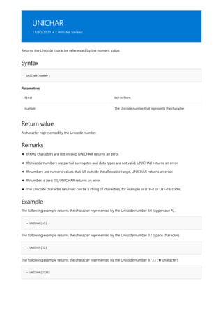
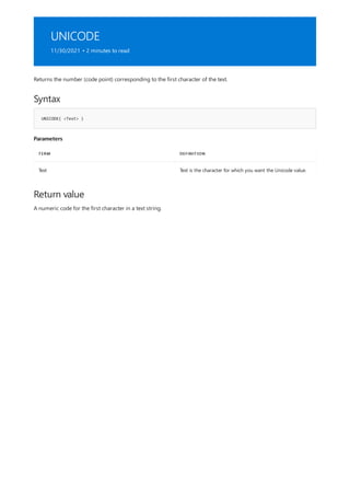
![UPPER
11/30/2021 • 2 minutes to read
Syntax
UPPER (<text>)
Parameters
TERM DEFINITION
text The text you want converted to uppercase, or a reference to
a column that contains text.
Return value
Example
= UPPER(['New Products'[Product Code])
See also
Converts a text string to all uppercase letters.
Same text, in uppercase.
The following formula converts the string in the column, [ProductCode], to all uppercase. Non-alphabetic
characters are not affected.
Text functions
LOWER function](https://image.slidesharecdn.com/funcoesdax-220812141017-bb6cd4dc/85/Funcoes-DAX-pdf-608-320.jpg)
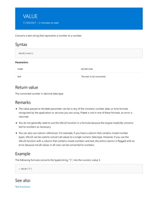
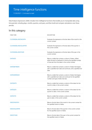
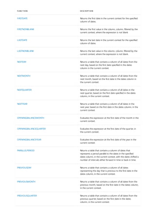
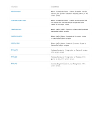
![CLOSINGBALANCEMONTH
11/30/2021 • 2 minutes to read
Syntax
CLOSINGBALANCEMONTH(<expression>,<dates>[,<filter>])
Parameters
PARAMETER DEFINITION
expression An expression that returns a scalar value.
dates A column that contains dates.
filter (optional) An expression that specifies a filter to apply to the
current context.
Return value
Remarks
Example
Evaluates the expression at the last date of the month in the current context.
A scalar value that represents the expression evaluated at the last date of the month in the current context.
The dates argument can be any of the following:
NOTE
NOTE
A reference to a date/time column.
A table expression that returns a single column of date/time values.
A Boolean expression that defines a single-column table of date/time values.
Constraints on Boolean expressions are described in CALCULATE function.
The filter expression has restrictions described in CALCULATE function.
This function is not supported for use in DirectQuery mode when used in calculated columns or row-
level security (RLS) rules.
The following sample formula creates a measure that calculates the 'Month End Inventory Value' of the product
inventory.](https://image.slidesharecdn.com/funcoesdax-220812141017-bb6cd4dc/85/Funcoes-DAX-pdf-613-320.jpg)
![=
CLOSINGBALANCEMONTH(SUMX(ProductInventory,ProductInventory[UnitCost]*ProductInventory[UnitsBalance]),DateTim
e[DateKey])
See also
Time intelligence functions
CLOSINGBALANCEYEAR function
CLOSINGBALANCEQUARTER function](https://image.slidesharecdn.com/funcoesdax-220812141017-bb6cd4dc/85/Funcoes-DAX-pdf-614-320.jpg)
![CLOSINGBALANCEQUARTER
11/30/2021 • 2 minutes to read
Syntax
CLOSINGBALANCEQUARTER(<expression>,<dates>[,<filter>])
Parameters
TERM DEFINITION
expression An expression that returns a scalar value.
dates A column that contains dates.
filter (optional) An expression that specifies a filter to apply to the
current context.
Return value
Remarks
Example
Evaluates the expression at the last date of the quarter in the current context.
A scalar value that represents the expression evaluated at the last date of the quarter in the current context.
The dates argument can be any of the following:
NOTE
NOTE
A reference to a date/time column.
A table expression that returns a single column of date/time values.
A Boolean expression that defines a single-column table of date/time values.
Constraints on Boolean expressions are described in CALCULATE function.
The filter expression has restrictions described in CALCULATE function.
This function is not supported for use in DirectQuery mode when used in calculated columns or row-
level security (RLS) rules.
The following sample formula creates a measure that calculates the 'Quarter End Inventory Value' of the product
inventory.](https://image.slidesharecdn.com/funcoesdax-220812141017-bb6cd4dc/85/Funcoes-DAX-pdf-615-320.jpg)
![=
CLOSINGBALANCEQUARTER(SUMX(ProductInventory,ProductInventory[UnitCost]*ProductInventory[UnitsBalance]),DateT
ime[DateKey])
See also
Time intelligence functions
CLOSINGBALANCEYEAR function
CLOSINGBALANCEMONTH function](https://image.slidesharecdn.com/funcoesdax-220812141017-bb6cd4dc/85/Funcoes-DAX-pdf-616-320.jpg)
![CLOSINGBALANCEYEAR
11/30/2021 • 2 minutes to read
Syntax
CLOSINGBALANCEYEAR(<expression>,<dates>[,<filter>][,<year_end_date>])
Parameters
TERM DEFINITION
expression An expression that returns a scalar value.
dates A column that contains dates.
filter (optional) An expression that specifies a filter to apply to the
current context.
year_end_date (optional) A literal string with a date that defines the year-
end date. The default is December 31.
Return value
Remarks
Evaluates the expression at the last date of the year in the current context.
A scalar value that represents the expression evaluated at the last date of the year in the current context.
The year_end_date parameter is a string literal of a date, in the same locale as the locale of the client
where the workbook was created. The year portion of the date is ignored.
The dates argument can be any of the following:
NOTE
NOTE
A reference to a date/time column.
A table expression that returns a single column of date/time values.
A Boolean expression that defines a single-column table of date/time values.
Constraints on Boolean expressions are described in CALCULATE function.
The filter expression has restrictions described in CALCULATE function.
This function is not supported for use in DirectQuery mode when used in calculated columns or row-
level security (RLS) rules.](https://image.slidesharecdn.com/funcoesdax-220812141017-bb6cd4dc/85/Funcoes-DAX-pdf-617-320.jpg)
![Example
=
CLOSINGBALANCEYEAR(SUMX(ProductInventory,ProductInventory[UnitCost]*ProductInventory[UnitsBalance]),DateTime
[DateKey])
See also
The following sample formula creates a measure that calculates the 'Year End Inventory Value' of the product
inventory.
Time intelligence functions
CLOSINGBALANCEYEAR function
CLOSINGBALANCEQUARTER function
CLOSINGBALANCEMONTH function](https://image.slidesharecdn.com/funcoesdax-220812141017-bb6cd4dc/85/Funcoes-DAX-pdf-618-320.jpg)
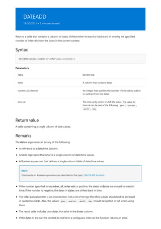
![Example - Shifting a set of dates
= DATEADD(DateTime[DateKey],-1,year)
See also
This function is not supported for use in DirectQuery mode when used in calculated columns or row-
level security (RLS) rules.
The following formula calculates dates that are one year before the dates in the current context.
Time intelligence functions
Date and time functions](https://image.slidesharecdn.com/funcoesdax-220812141017-bb6cd4dc/85/Funcoes-DAX-pdf-620-320.jpg)
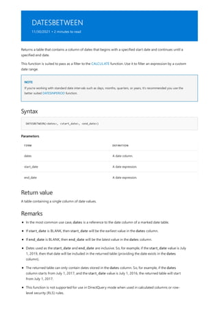
![Example
Customers LTD =
CALCULATE(
DISTINCTCOUNT(Sales[CustomerKey]),
DATESBETWEEN(
'Date'[Date],
BLANK(),
MAX('Date'[Date])
)
)
See also
The following Sales table measure definition uses the DATESBETWEEN function to produce a life-to-date (LTD)
calculation. Life-to-date represents the accumulation of a measure over time since the very beginning of time.
Notice that the formula uses the MAX function. This function returns the latest date that's in the filter context. So,
the DATESBETWEEN function returns a table of dates beginning from the earliest date until the latest date being
reported.
Examples in this article can be added to the Power BI Desktop sample model. To get the model, see DAX sample
model.
Consider that the earliest date stored in the Date table is July 1, 2017. So, when a report filters the measure by
the month of June 2020, the DATESBETWEEN function returns a date range from July 1, 2017 until June 30,
2020.
Time intelligence functions (DAX)
Date and time functions (DAX)
DATESINPERIOD function (DAX)](https://image.slidesharecdn.com/funcoesdax-220812141017-bb6cd4dc/85/Funcoes-DAX-pdf-622-320.jpg)
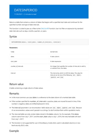
![Revenue PY =
CALCULATE(
SUM(Sales[Sales Amount]),
DATESINPERIOD(
'Date'[Date],
MAX('Date'[Date]),
-1,
YEAR
)
)
See also
The following Sales table measure definition uses the DATESINPERIOD function to calculate revenue for the
prior year (PY).
Notice the formula uses the MAX function. This function returns the latest date that's in the filter context. So, the
DATESINPERIOD function returns a table of dates beginning from the latest date for the last year.
Examples in this article can be added to the Power BI Desktop sample model. To get the model, see DAX sample
model.
Consider that the report is filtered by the month of June 2020. The MAX function returns June 30, 2020. The
DATESINPERIOD function then returns a date range from July 1, 2019 until June 30, 2020. It's a year of date
values starting from June 30, 2020 for the last year.
Time intelligence functions (DAX)
Date and time functions (DAX)
DATESBETWEEN function (DAX)](https://image.slidesharecdn.com/funcoesdax-220812141017-bb6cd4dc/85/Funcoes-DAX-pdf-624-320.jpg)
![DATESMTD
11/30/2021 • 2 minutes to read
Syntax
DATESMTD(<dates>)
Parameters
TERM DEFINITION
dates A column that contains dates.
Return value
Remarks
Example
= CALCULATE(SUM(InternetSales_USD[SalesAmount_USD]), DATESMTD(DateTime[DateKey]))
See also
Returns a table that contains a column of the dates for the month to date, in the current context.
A table containing a single column of date values.
The dates argument can be any of the following:
NOTE
A reference to a date/time column.
A table expression that returns a single column of date/time values.
A Boolean expression that defines a single-column table of date/time values.
Constraints on Boolean expressions are described in the topic, CALCULATE function.
This function is not supported for use in DirectQuery mode when used in calculated columns or row-
level security (RLS) rules.
The following sample formula creates a measure that calculates the 'Month To Date Total' for Internet Sales.
Time intelligence functions
Date and time functions
DATESYTD function
DATESQTD function](https://image.slidesharecdn.com/funcoesdax-220812141017-bb6cd4dc/85/Funcoes-DAX-pdf-625-320.jpg)
![DATESQTD
11/30/2021 • 2 minutes to read
Syntax
DATESQTD(<dates>)
Parameters
TERM DEFINITION
dates A column that contains dates.
Return value
Remarks
Example
= CALCULATE(SUM(InternetSales_USD[SalesAmount_USD]), DATESQTD(DateTime[DateKey]))
See also
Returns a table that contains a column of the dates for the quarter to date, in the current context.
A table containing a single column of date values.
The dates argument can be any of the following:
NOTE
A reference to a date/time column.
A table expression that returns a single column of date/time values.
A Boolean expression that defines a single-column table of date/time values.
Constraints on Boolean expressions are described in the topic, CALCULATE function.
This function is not supported for use in DirectQuery mode when used in calculated columns or row-
level security (RLS) rules.
The following sample formula creates a measure that calculates the 'Quarterly Running Total' of Internet Sales.
Time intelligence functions
Date and time functions
DATESYTD function
DATESMTD function](https://image.slidesharecdn.com/funcoesdax-220812141017-bb6cd4dc/85/Funcoes-DAX-pdf-626-320.jpg)
![DATESYTD
11/30/2021 • 2 minutes to read
Syntax
DATESYTD(<dates> [,<year_end_date>])
Parameters
TERM DEFINITION
dates A column that contains dates.
year_end_date (optional) A literal string with a date that defines the year-
end date. The default is December 31.
Return value
Remarks
Example
= CALCULATE(SUM(InternetSales_USD[SalesAmount_USD]), DATESYTD(DateTime[DateKey]))
See also
Returns a table that contains a column of the dates for the year to date, in the current context.
A table containing a single column of date values.
The dates argument can be any of the following:
NOTE
A reference to a date/time column,
A table expression that returns a single column of date/time values,
A Boolean expression that defines a single-column table of date/time values.
Constraints on Boolean expressions are described in the topic, CALCULATE function.
The year_end_date parameter is a string literal of a date, in the same locale as the locale of the client
where the workbook was created. The year portion of the date is ignored.
This function is not supported for use in DirectQuery mode when used in calculated columns or row-
level security (RLS) rules.
The following sample formula creates a measure that calculates the 'Running Total' for Internet sales.](https://image.slidesharecdn.com/funcoesdax-220812141017-bb6cd4dc/85/Funcoes-DAX-pdf-627-320.jpg)

![ENDOFMONTH
11/30/2021 • 2 minutes to read
Syntax
ENDOFMONTH(<dates>)
Parameters
TERM DEFINITION
dates A column that contains dates.
Return value
Remarks
Example
= ENDOFMONTH(DateTime[DateKey])
See also
Returns the last date of the month in the current context for the specified column of dates.
A table containing a single column and single row with a date value.
The dates argument can be any of the following:
A reference to a date/time column.
A table expression that returns a single column of date/time values.
A Boolean expression that defines a single-column table of date/time values.
Constraints on Boolean expressions are described in the topic, CALCULATE function.
This function is not supported for use in DirectQuery mode when used in calculated columns or row-
level security (RLS) rules.
The following sample formula creates a measure that returns the end of the month, for the current context.
Date and time functions
Time intelligence functions
ENDOFYEAR function
ENDOFQUARTER function](https://image.slidesharecdn.com/funcoesdax-220812141017-bb6cd4dc/85/Funcoes-DAX-pdf-629-320.jpg)
![ENDOFQUARTER
11/30/2021 • 2 minutes to read
Syntax
ENDOFQUARTER(<dates>)
Parameters
TERM DEFINITION
dates A column that contains dates.
Return value
Remarks
Example
= ENDOFQUARTER(DateTime[DateKey])
See also
Returns the last date of the quarter in the current context for the specified column of dates.
A table containing a single column and single row with a date value.
The dates argument can be any of the following:
A reference to a date/time column,
A table expression that returns a single column of date/time values,
A Boolean expression that defines a single-column table of date/time values.
Constraints on Boolean expressions are described in the topic, CALCULATE function.
This function is not supported for use in DirectQuery mode when used in calculated columns or row-
level security (RLS) rules.
The following sample formula creates a measure that returns the end of the quarter, for the current context.
Date and time functions
Time intelligence functions
ENDOFYEAR function
ENDOFMONTH function](https://image.slidesharecdn.com/funcoesdax-220812141017-bb6cd4dc/85/Funcoes-DAX-pdf-630-320.jpg)
![ENDOFYEAR
11/30/2021 • 2 minutes to read
Syntax
ENDOFYEAR(<dates> [,<year_end_date>])
Parameters
TERM DEFINITION
dates A column that contains dates.
year_end_date (optional) A literal string with a date that defines the year-
end date. The default is December 31.
Return value
Remarks
Example
= ENDOFYEAR(DateTime[DateKey],"06/30/2004")
See also
Returns the last date of the year in the current context for the specified column of dates.
A table containing a single column and single row with a date value.
The dates argument can be any of the following:
A reference to a date/time column,
A table expression that returns a single column of date/time values,
A Boolean expression that defines a single-column table of date/time values.
Constraints on Boolean expressions are described in the topic, CALCULATE function.
The year_end_date parameter is a string literal of a date, in the same locale as the locale of the client
where the workbook was created. The year portion of the date is ignored.
This function is not supported for use in DirectQuery mode when used in calculated columns or row-
level security (RLS) rules.
The following sample formula creates a measure that returns the end of the fiscal year that ends on June 30, for
the current context.
Date and time functions
Time intelligence functions
ENDOFMONTH function](https://image.slidesharecdn.com/funcoesdax-220812141017-bb6cd4dc/85/Funcoes-DAX-pdf-631-320.jpg)

![FIRSTDATE
11/30/2021 • 2 minutes to read
Syntax
FIRSTDATE(<dates>)
Parameters
TERM DEFINITION
dates A column that contains dates.
Return value
Remarks
Example
= FIRSTDATE('InternetSales_USD'[SaleDateKey])
See also
Returns the first date in the current context for the specified column of dates.
A table containing a single column and single row with a date value.
The dates argument can be any of the following:
A reference to a date/time column.
A table expression that returns a single column of date/time values.
A Boolean expression that defines a single-column table of date/time values.
Constraints on Boolean expressions are described in the topic, CALCULATE function.
When the current context is a single date, the date returned by the FIRSTDATE and LASTDATE functions
will be equal.
The Return value is a table that contains a single column and single value. Therefore, this function can be
used as an argument to any function that requires a table in its arguments. Also, the returned value can
be used whenever a date value is required.
This function is not supported for use in DirectQuery mode when used in calculated columns or row-
level security (RLS) rules.
The following sample formula creates a measure that obtains the first date when a sale was made in the Internet
sales channel for the current context.
Date and time functions
Time intelligence functions](https://image.slidesharecdn.com/funcoesdax-220812141017-bb6cd4dc/85/Funcoes-DAX-pdf-633-320.jpg)

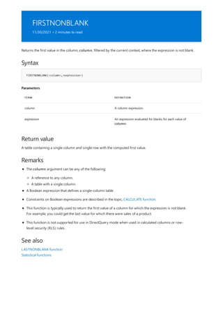
![FIRSTNONBLANKVALUE
11/30/2021 • 2 minutes to read
Syntax
FIRSTNONBLANKVALUE(<column>, <expression>)
Parameters
TERM DEFINITION
column A column or an expression that returns a single-column
table.
expression An expression evaluated for each value of <column>.
Return value
Remarks
Example
EVALUATE
SUMMARIZECOLUMNS(
DimProduct[Class],
"FNBV",
FIRSTNONBLANKVALUE(
DimDate[Date],
SUM(FactInternetSales[SalesAmount])
)
)
Evaluates an expression filtered by the sorted values of a column and returns the first value of the expression
that is not blank.
The first non-blank value of <expression> corresponding to the sorted values of <column>.
The column argument can be any of the following:
A reference to any column.
A table with a single column.
This function is different from FIRSTNONBLANK in that the <column> is added to the filter context for
the evaluation of <expression>.
This function is not supported for use in DirectQuery mode when used in calculated columns or row-
level security (RLS) rules.
The following DAX query,
Returns,](https://image.slidesharecdn.com/funcoesdax-220812141017-bb6cd4dc/85/Funcoes-DAX-pdf-636-320.jpg)
![DIMPRODUCT[CLASS] [FNBV]
L 699.0982
H 13778.24
M 1000.4375
533.83](https://image.slidesharecdn.com/funcoesdax-220812141017-bb6cd4dc/85/Funcoes-DAX-pdf-637-320.jpg)
![LASTDATE
11/30/2021 • 2 minutes to read
Syntax
LASTDATE(<dates>)
Parameters
TERM DEFINITION
dates A column that contains dates.
Return value
Remarks
Example
= LASTDATE('InternetSales_USD'[SaleDateKey])
See also
Returns the last date in the current context for the specified column of dates.
A table containing a single column and single row with a date value.
The dates argument can be any of the following:
A reference to a date/time column,
A table expression that returns a single column of date/time values,
A Boolean expression that defines a single-column table of date/time values.
Constraints on Boolean expressions are described in the topic, CALCULATE function.
When the current context is a single date, the date returned by the FIRSTDATE and LASTDATE functions
will be equal.
Technically, the Return value is a table that contains a single column and single value. Therefore, this
function can be used as an argument to any function that requires a table in its arguments. Also, the
returned value can be used whenever a date value is required.
This function is not supported for use in DirectQuery mode when used in calculated columns or row-
level security (RLS) rules.
The following sample formula creates a measure that obtains the last date, for the current context, when a sale
was made in the Internet sales channel.
Date and time functions
Time intelligence functions](https://image.slidesharecdn.com/funcoesdax-220812141017-bb6cd4dc/85/Funcoes-DAX-pdf-638-320.jpg)

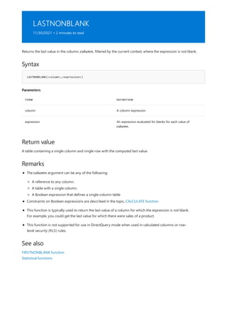
![LASTNONBLANKVALUE
11/30/2021 • 2 minutes to read
Syntax
LASTNONBLANKVALUE(<column>, <expression>)
Parameters
TERM DEFINITION
column A column or an expression that returns a single-column
table.
expression An expression evaluated for each value of <column>.
Return value
Remarks
Example
EVALUATE
SUMMARIZECOLUMNS(
DimProduct[Class],
"LNBV",
LASTNONBLANKVALUE(
DimDate[Date],
SUM(FactInternetSales[SalesAmount])
)
)
Evaluates an expression filtered by the sorted values of a column and returns the last value of the expression
that is not blank.
The last non-blank value of <expression> corresponding to the sorted values of <column>.
The column argument can be any of the following:
A reference to any column.
A table with a single column.
This function is different from LASTNONBLANK in that the <column> is added to the filter context for the
evaluation of <expression>.
This function is not supported for use in DirectQuery mode when used in calculated columns or row-
level security (RLS) rules.
The following DAX query,
Returns,](https://image.slidesharecdn.com/funcoesdax-220812141017-bb6cd4dc/85/Funcoes-DAX-pdf-641-320.jpg)
![DIMPRODUCT[CLASS] [LNBV]
L 132.44
H 137.6
M 84.97
2288.6](https://image.slidesharecdn.com/funcoesdax-220812141017-bb6cd4dc/85/Funcoes-DAX-pdf-642-320.jpg)
![NEXTDAY
11/30/2021 • 2 minutes to read
Syntax
NEXTDAY(<dates>)
Parameters
TERM DEFINITION
dates A column containing dates.
Return value
Remarks
Example
= CALCULATE(SUM(InternetSales_USD[SalesAmount_USD]), NEXTDAY('DateTime'[DateKey]))
See also
Returns a table that contains a column of all dates from the next day, based on the first date specified in the
dates column in the current context.
A table containing a single column of date values.
This function returns all dates from the next day to the first date in the input parameter. For example, if
the first date in the dates argument refers to June 10, 2009; then this function returns all dates equal to
June 11, 2009.
The dates argument can be any of the following:
A reference to a date/time column.
A table expression that returns a single column of date/time values.
A Boolean expression that defines a single-column table of date/time values.
Constraints on Boolean expressions are described in the topic, CALCULATE function.
This function is not supported for use in DirectQuery mode when used in calculated columns or row-
level security (RLS) rules.
The following sample formula creates a measure that calculates the 'next day sales' of Internet sales.
Time intelligence functions
Date and time functions
NEXTQUARTER function
NEXTMONTH function](https://image.slidesharecdn.com/funcoesdax-220812141017-bb6cd4dc/85/Funcoes-DAX-pdf-643-320.jpg)

![NEXTMONTH
11/30/2021 • 2 minutes to read
Syntax
NEXTMONTH(<dates>)
Parameters
TERM DEFINITION
dates A column containing dates.
Return value
Remarks
Example
= CALCULATE(SUM(InternetSales_USD[SalesAmount_USD]), NEXTMONTH('DateTime'[DateKey]))
See also
Returns a table that contains a column of all dates from the next month, based on the first date in the dates
column in the current context.
A table containing a single column of date values.
This function returns all dates from the next day to the first date in the input parameter. For example, if
the first date in the dates argument refers to June 10, 2009; then this function returns all dates for the
month of July, 2009.
The dates argument can be any of the following:
A reference to a date/time column.
A table expression that returns a single column of date/time values.
A Boolean expression that defines a single-column table of date/time values.
Constraints on Boolean expressions are described in the topic, CALCULATE function.
This function is not supported for use in DirectQuery mode when used in calculated columns or row-
level security (RLS) rules.
The following sample formula creates a measure that calculates the 'next month sales' for Internet sales.
Time intelligence functions
Date and time functions
NEXTDAY function
NEXTQUARTER function](https://image.slidesharecdn.com/funcoesdax-220812141017-bb6cd4dc/85/Funcoes-DAX-pdf-645-320.jpg)

![NEXTQUARTER
11/30/2021 • 2 minutes to read
Syntax
NEXTQUARTER(<dates>)
Parameters
TERM DEFINITION
dates A column containing dates.
Return value
Remarks
Example
= CALCULATE(SUM(InternetSales_USD[SalesAmount_USD]), NEXTQUARTER('DateTime'[DateKey]))
See also
Returns a table that contains a column of all dates in the next quarter, based on the first date specified in the
dates column, in the current context.
A table containing a single column of date values.
This function returns all dates in the next quarter, based on the first date in the input parameter. For
example, if the first date in the dates column refers to June 10, 2009, this function returns all dates for
the quarter July to September, 2009.
The dates argument can be any of the following:
A reference to a date/time column.
A table expression that returns a single column of date/time values.
A Boolean expression that defines a single-column table of date/time values.
Constraints on Boolean expressions are described in the topic, CALCULATE function.
This function is not supported for use in DirectQuery mode when used in calculated columns or row-
level security (RLS) rules.
The following sample formula creates a measure that calculates the 'next quarter sales' for Internet sales.
Time intelligence functions
Date and time functions
NEXTDAY function
NEXTMONTH function](https://image.slidesharecdn.com/funcoesdax-220812141017-bb6cd4dc/85/Funcoes-DAX-pdf-647-320.jpg)

![NEXTYEAR
11/30/2021 • 2 minutes to read
Syntax
NEXTYEAR(<dates>[,<year_end_date>])
Parameters
TERM DEFINITION
dates A column containing dates.
year_end_date (optional) A literal string with a date that defines the year-
end date. The default is December 31.
Return value
Remarks
Example
= CALCULATE(SUM(InternetSales_USD[SalesAmount_USD]), NEXTYEAR('DateTime'[DateKey]))
Returns a table that contains a column of all dates in the next year, based on the first date in the dates column,
in the current context.
A table containing a single column of date values.
This function returns all dates in the next year, based on the first date in the input column. For example, if
the first date in the dates column refers to the year 2007, this function returns all dates for the year
2008.
The dates argument can be any of the following:
A reference to a date/time column.
A table expression that returns a single column of date/time values.
A Boolean expression that defines a single-column table of date/time values.
Constraints on Boolean expressions are described in the topic, CALCULATE function.
The year_end_date parameter is a string literal of a date, in the same locale as the locale of the client
where the workbook was created. The year portion of the date is ignored.
This function is not supported for use in DirectQuery mode when used in calculated columns or row-
level security (RLS) rules.
The following sample formula creates a measure that calculates the 'next year sales' for Internet sales.](https://image.slidesharecdn.com/funcoesdax-220812141017-bb6cd4dc/85/Funcoes-DAX-pdf-649-320.jpg)

![OPENINGBALANCEMONTH
11/30/2021 • 2 minutes to read
Syntax
OPENINGBALANCEMONTH(<expression>,<dates>[,<filter>])
Parameters
TERM DEFINITION
expression An expression that returns a scalar value.
dates A column that contains dates.
filter (optional) An expression that specifies a filter to apply to the
current context.
Return value
Remarks
Example
=
OPENINGBALANCEMONTH(SUMX(ProductInventory,ProductInventory[UnitCost]*ProductInventory[UnitsBalance]),DateTim
e[DateKey])
See also
Evaluates the expression at the first date of the month in the current context.
A scalar value that represents the expression evaluated at the first date of the month in the current context.
The dates argument can be any of the following:
A reference to a date/time column.
A table expression that returns a single column of date/time values.
A Boolean expression that defines a single-column table of date/time values.
Constraints on Boolean expressions are described in the topic, CALCULATE function.
The filter expression has restrictions described in the topic, CALCULATE function.
This function is not supported for use in DirectQuery mode when used in calculated columns or row-
level security (RLS) rules.
The following sample formula creates a measure that calculates the 'Month Start Inventory Value' of the product
inventory.](https://image.slidesharecdn.com/funcoesdax-220812141017-bb6cd4dc/85/Funcoes-DAX-pdf-651-320.jpg)

![OPENINGBALANCEQUARTER
11/30/2021 • 2 minutes to read
Syntax
OPENINGBALANCEQUARTER(<expression>,<dates>[,<filter>])
Parameters
TERM DEFINITION
expression An expression that returns a scalar value.
dates A column that contains dates.
filte* (optional) An expression that specifies a filter to apply to the
current context.
Return value
Remarks
Example
=
OPENINGBALANCEQUARTER(SUMX(ProductInventory,ProductInventory[UnitCost]*ProductInventory[UnitsBalance]),DateT
ime[DateKey])
See also
Evaluates the expression at the first date of the quarter, in the current context.
A scalar value that represents the expression evaluated at the first date of the quarter in the current context.
The dates argument can be any of the following:
A reference to a date/time column.
A table expression that returns a single column of date/time values.
A Boolean expression that defines a single-column table of date/time values.
Constraints on Boolean expressions are described in the topic, CALCULATE function.
The filter expression has restrictions described in the topic, CALCULATE function.
This function is not supported for use in DirectQuery mode when used in calculated columns or row-
level security (RLS) rules.
The following sample formula creates a measure that calculates the 'Quarter Start Inventory Value' of the
product inventory.](https://image.slidesharecdn.com/funcoesdax-220812141017-bb6cd4dc/85/Funcoes-DAX-pdf-653-320.jpg)

![OPENINGBALANCEYEAR
11/30/2021 • 2 minutes to read
Syntax
OPENINGBALANCEYEAR(<expression>,<dates>[,<filter>][,<year_end_date>])
Parameters
TERM DEFINITION
expression An expression that returns a scalar value.
dates A column that contains dates.
filter (optional) An expression that specifies a filter to apply to the
current context.
year_end_date (optional) A literal string with a date that defines the year-
end date. The default is December 31.
Return value
Remarks
Example
Evaluates the expression at the first date of the year in the current context.
A scalar value that represents the expression evaluated at the first date of the year in the current context.
The dates argument can be any of the following:
A reference to a date/time column.
A table expression that returns a single column of date/time values.
A Boolean expression that defines a single-column table of date/time values.
Constraints on Boolean expressions are described in the topic, CALCULATE function.
The filter expression has restrictions described in the topic, CALCULATE function.
The year_end_date parameter is a string literal of a date, in the same locale as the locale of the client
where the workbook was created. The year portion of the date is ignored.
This function is not supported for use in DirectQuery mode when used in calculated columns or row-
level security (RLS) rules.
The following sample formula creates a measure that calculates the 'Year Start Inventory Value' of the product
inventory.](https://image.slidesharecdn.com/funcoesdax-220812141017-bb6cd4dc/85/Funcoes-DAX-pdf-655-320.jpg)
![=
OPENINGBALANCEYEAR(SUMX(ProductInventory,ProductInventory[UnitCost]*ProductInventory[UnitsBalance]),DateTime
[DateKey])
See also
OPENINGBALANCEQUARTER function
OPENINGBALANCEMONTH function
Time intelligence functions
CLOSINGBALANCEYEAR function](https://image.slidesharecdn.com/funcoesdax-220812141017-bb6cd4dc/85/Funcoes-DAX-pdf-656-320.jpg)
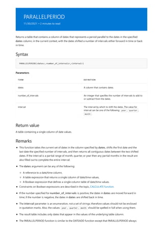
![Example
= CALCULATE(SUM(InternetSales_USD[SalesAmount_USD]), PARALLELPERIOD(DateTime[DateKey],-1,year))
See also
returns full periods at the given granularity level instead of the partial periods that DATEADD returns. For
example, if you have a selection of dates that starts at June 10 and finishes at June 21 of the same year,
and you want to shift that selection forward by one month then the PARALLELPERIOD function will return
all dates from the next month (July 1 to July 31); however, if DATEADD is used instead, then the result will
include only dates from July 10 to July 21.
This function is not supported for use in DirectQuery mode when used in calculated columns or row-
level security (RLS) rules.
The following sample formula creates a measure that calculates the previous year sales for Internet sales.
Time intelligence functions
Date and time functions
DATEADD function](https://image.slidesharecdn.com/funcoesdax-220812141017-bb6cd4dc/85/Funcoes-DAX-pdf-658-320.jpg)
![PREVIOUSDAY
11/30/2021 • 2 minutes to read
Syntax
PREVIOUSDAY(<dates>)
Parameters
TERM DEFINITION
dates A column containing dates.
Return value
Remarks
Example
= CALCULATE(SUM(InternetSales_USD[SalesAmount_USD]), PREVIOUSDAY('DateTime'[DateKey]))
See also
Returns a table that contains a column of all dates representing the day that is previous to the first date in the
dates column, in the current context.
A table containing a single column of date values.
This function determines the first date in the input parameter, and then returns all dates corresponding to
the day previous to that first date. For example, if the first date in the dates argument refers to June 10,
2009; this function returns all dates equal to June 9, 2009.
The dates argument can be any of the following:
A reference to a date/time column.
A table expression that returns a single column of date/time values.
A Boolean expression that defines a single-column table of date/time values.
Constraints on Boolean expressions are described in the topic, CALCULATE function.
This function is not supported for use in DirectQuery mode when used in calculated columns or row-
level security (RLS) rules.
The following sample formula creates a measure that calculates the 'previous day sales' for Internet sales.
Time intelligence functions
Date and time functions
PREVIOUSMONTH function
PREVIOUSQUARTER function](https://image.slidesharecdn.com/funcoesdax-220812141017-bb6cd4dc/85/Funcoes-DAX-pdf-659-320.jpg)

![PREVIOUSMONTH
11/30/2021 • 2 minutes to read
Syntax
PREVIOUSMONTH(<dates>)
Parameters
TERM DEFINITION
Dates A column containing dates.
Return value
Remarks
Example
= CALCULATE(SUM(InternetSales_USD[SalesAmount_USD]), PREVIOUSMONTH('DateTime'[DateKey]))
See also
Returns a table that contains a column of all dates from the previous month, based on the first date in the dates
column, in the current context.
A table containing a single column of date values.
This function returns all dates from the previous month, using the first date in the column used as input.
For example, if the first date in the dates argument refers to June 10, 2009, this function returns all dates
for the month of May, 2009.
The dates argument can be any of the following:
A reference to a date/time column.
A table expression that returns a single column of date/time values.
A Boolean expression that defines a single-column table of date/time values.
Constraints on Boolean expressions are described in the topic, CALCULATE.
This function is not supported for use in DirectQuery mode when used in calculated columns or row-
level security (RLS) rules.
The following sample formula creates a measure that calculates the 'previous month sales' for Internet sales.
Time intelligence functions
Date and time functions
PREVIOUSDAY
PREVIOUSQUARTER](https://image.slidesharecdn.com/funcoesdax-220812141017-bb6cd4dc/85/Funcoes-DAX-pdf-661-320.jpg)

![PREVIOUSQUARTER
11/30/2021 • 2 minutes to read
Syntax
PREVIOUSQUARTER(<dates>)
Parameters
TERM DEFINITION
dates A column containing dates.
Return value
Remarks
Example
= CALCULATE(SUM(InternetSales_USD[SalesAmount_USD]), PREVIOUSQUARTER('DateTime'[DateKey]))
See also
Returns a table that contains a column of all dates from the previous quarter, based on the first date in the dates
column, in the current context.
A table containing a single column of date values.
This function returns all dates from the previous quarter, using the first date in the input column. For
example, if the first date in the dates argument refers to June 10, 2009, this function returns all dates for
the quarter January to March, 2009.
The dates argument can be any of the following:
A reference to a date/time column.
A table expression that returns a single column of date/time values.
A Boolean expression that defines a single-column table of date/time values.
Constraints on Boolean expressions are described in the topic, CALCULATE.
This function is not supported for use in DirectQuery mode when used in calculated columns or row-
level security (RLS) rules.
The following sample formula creates a measure that calculates the 'previous quarter sales' for Internet sales.
Time intelligence functions
Date and time functions
PREVIOUSMONTH
PREVIOUSDAY](https://image.slidesharecdn.com/funcoesdax-220812141017-bb6cd4dc/85/Funcoes-DAX-pdf-663-320.jpg)

![PREVIOUSYEAR
11/30/2021 • 2 minutes to read
Syntax
PREVIOUSYEAR(<dates>[,<year_end_date>])
Parameters
TERM DEFINITION
dates A column containing dates.
year_end_date (optional) A literal string with a date that defines the year-
end date. The default is December 31.
Return value
Remarks
Example
= CALCULATE(SUM(InternetSales_USD[SalesAmount_USD]), PREVIOUSYEAR('DateTime'[DateKey]))
Returns a table that contains a column of all dates from the previous year, given the last date in the dates
column, in the current context.
A table containing a single column of date values.
This function returns all dates from the previous year given the latest date in the input parameter. For
example, if the latest date in the dates argument refers to the year 2009, then this function returns all
dates for the year of 2008, up to the specified year_end_date.
The dates argument can be any of the following:
A reference to a date/time column.
A table expression that returns a single column of date/time values.
A Boolean expression that defines a single-column table of date/time values.
Constraints on Boolean expressions are described in the topic, CALCULATE.
The year_end_date parameter is a string literal of a date, in the same locale as the locale of the client
where the workbook was created. The year portion of the date is ignored.
This function is not supported for use in DirectQuery mode when used in calculated columns or row-
level security (RLS) rules.
The following sample formula creates a measure that calculates the previous year sales for Internet sales.](https://image.slidesharecdn.com/funcoesdax-220812141017-bb6cd4dc/85/Funcoes-DAX-pdf-665-320.jpg)

![SAMEPERIODLASTYEAR
11/30/2021 • 2 minutes to read
Syntax
SAMEPERIODLASTYEAR(<dates>)
Parameters
TERM DEFINITION
dates A column containing dates.
Return value
Remarks
Example
= CALCULATE(SUM(ResellerSales_USD[SalesAmount_USD]), SAMEPERIODLASTYEAR(DateTime[DateKey]))
See also
Returns a table that contains a column of dates shifted one year back in time from the dates in the specified
dates column, in the current context.
A single-column table of date values.
The dates argument can be any of the following:
A reference to a date/time column,
A table expression that returns a single column of date/time values,
A Boolean expression that defines a single-column table of date/time values.
Constraints on Boolean expressions are described in the topic, CALCULATE.
The dates returned are the same as the dates returned by this equivalent formula:
DATEADD(dates, -1, year)
This function is not supported for use in DirectQuery mode when used in calculated columns or row-
level security (RLS) rules.
The following sample formula creates a measure that calculates the previous year sales of Reseller sales.
Time intelligence functions
Date and time functions
PREVIOUSYEAR
PARALLELPERIOD](https://image.slidesharecdn.com/funcoesdax-220812141017-bb6cd4dc/85/Funcoes-DAX-pdf-667-320.jpg)
![STARTOFMONTH
11/30/2021 • 2 minutes to read
Syntax
STARTOFMONTH(<dates>)
Parameters
TERM DEFINITION
dates A column that contains dates.
Return value
Remarks
Example
= STARTOFMONTH(DateTime[DateKey])
See also
Returns the first date of the month in the current context for the specified column of dates.
A table containing a single column and single row with a date value.
The dates argument can be any of the following:
A reference to a date/time column.
A table expression that returns a single column of date/time values.
A Boolean expression that defines a single-column table of date/time values.
Constraints on Boolean expressions are described in the topic, CALCULATE.
This function is not supported for use in DirectQuery mode when used in calculated columns or row-
level security (RLS) rules.
The following sample formula creates a measure that returns the start of the month, for the current context.
Date and time functions
Time intelligence functions
STARTOFYEAR
STARTOFQUARTER](https://image.slidesharecdn.com/funcoesdax-220812141017-bb6cd4dc/85/Funcoes-DAX-pdf-668-320.jpg)
![STARTOFQUARTER
11/30/2021 • 2 minutes to read
Syntax
STARTOFQUARTER(<dates>)
Parameters
TERM DEFINITION
dates A column that contains dates.
Return value
Remarks
Example
= STARTOFQUARTER(DateTime[DateKey])
See also
Returns the first date of the quarter in the current context for the specified column of dates.
A table containing a single column and single row with a date value.
The dates argument can be any of the following:
A reference to a date/time column.
A table expression that returns a single column of date/time values.
A Boolean expression that defines a single-column table of date/time values.
Constraints on Boolean expressions are described in the topic, CALCULATE.
This function is not supported for use in DirectQuery mode when used in calculated columns or row-
level security (RLS) rules.
The following sample formula creates a measure that returns the start of the quarter, for the current context.
Date and time functions
Time intelligence functions
STARTOFYEAR
STARTOFMONTH](https://image.slidesharecdn.com/funcoesdax-220812141017-bb6cd4dc/85/Funcoes-DAX-pdf-669-320.jpg)
![STARTOFYEAR
11/30/2021 • 2 minutes to read
Syntax
STARTOFYEAR(<dates>)
Parameters
TERM DEFINITION
dates A column that contains dates.
YearEndDate (Optional) A year end date value.
Return value
Remarks
Example
= STARTOFYEAR(DateTime[DateKey])
See also
Returns the first date of the year in the current context for the specified column of dates.
A table containing a single column and single row with a date value.
The dates argument can be any of the following:
A reference to a date/time column.
A table expression that returns a single column of date/time values.
A Boolean expression that defines a single-column table of date/time values.
Constraints on Boolean expressions are described in the topic, CALCULATE.
This function is not supported for use in DirectQuery mode when used in calculated columns or row-
level security (RLS) rules.
The following sample formula creates a measure that returns the start of the year, for the current context.
Date and time functions
Time intelligence functions
STARTOFQUARTER
STARTOFMONTH](https://image.slidesharecdn.com/funcoesdax-220812141017-bb6cd4dc/85/Funcoes-DAX-pdf-670-320.jpg)
![TOTALMTD
11/30/2021 • 2 minutes to read
Syntax
TOTALMTD(<expression>,<dates>[,<filter>])
Parameters
PARAMETER DEFINITION
expression An expression that returns a scalar value.
dates A column that contains dates.
filter (optional) An expression that specifies a filter to apply to the
current context.
Return value
Remarks
Example
= TOTALMTD(SUM(InternetSales_USD[SalesAmount_USD]),DateTime[DateKey])
See also
Evaluates the value of the expression for the month to date, in the current context.
A scalar value that represents the expression evaluated for the dates in the current month-to-date, given the
dates in dates.
The dates argument can be any of the following:
A reference to a date/time column.
A table expression that returns a single column of date/time values.
A Boolean expression that defines a single-column table of date/time values.
Constraints on Boolean expressions are described in the topic, CALCULATE.
The filter expression has restrictions described in the topic, CALCULATE.
This function is not supported for use in DirectQuery mode when used in calculated columns or row-
level security (RLS) rules.
The following sample formula creates a measure that calculates the 'month running total' or 'month running
sum' for Internet sales.
ALL](https://image.slidesharecdn.com/funcoesdax-220812141017-bb6cd4dc/85/Funcoes-DAX-pdf-671-320.jpg)

![TOTALQTD
11/30/2021 • 2 minutes to read
Syntax
TOTALQTD(<expression>,<dates>[,<filter>])
Parameters
PARAMETER DEFINITION
expression An expression that returns a scalar value.
dates A column that contains dates.
filter (optional) An expression that specifies a filter to apply to the
current context.
Return value
Remarks
Example
= TOTALQTD(SUM(InternetSales_USD[SalesAmount_USD]),DateTime[DateKey])
See also
Evaluates the value of the expression for the dates in the quarter to date, in the current context.
A scalar value that represents the expression evaluated for all dates in the current quarter to date, given the
dates in dates.
The dates argument can be any of the following:
A reference to a date/time column.
A table expression that returns a single column of date/time values.
A Boolean expression that defines a single-column table of date/time values.
Constraints on Boolean expressions are described in the topic, CALCULATE.
The filter expression has restrictions described in the topic, CALCULATE.
This function is not supported for use in DirectQuery mode when used in calculated columns or row-
level security (RLS) rules.
The following sample formula creates a measure that calculates the 'quarter running total' or 'quarter running
sum' for Internet sales.
ALL](https://image.slidesharecdn.com/funcoesdax-220812141017-bb6cd4dc/85/Funcoes-DAX-pdf-673-320.jpg)

![TOTALYTD
11/30/2021 • 2 minutes to read
Syntax
TOTALYTD(<expression>,<dates>[,<filter>][,<year_end_date>])
Parameters
PARAMETER DEFINITION
expression An expression that returns a scalar value.
dates A column that contains dates.
filter (optional) An expression that specifies a filter to apply to the
current context.
year_end_date (optional) A literal string with a date that defines the year-
end date. The default is December 31.
Return value
Remarks
Evaluates the year-to-date value of the expression in the current context.
A scalar value that represents the expression evaluated for the current year-to-date dates.
= TOTALYTD(SUM(InternetSales_USD[SalesAmount_USD]),DateTime[DateKey], ALL('DateTime'), "6/30")
The dates argument can be any of the following:
A reference to a date/time column.
A table expression that returns a single column of date/time values.
A Boolean expression that defines a single-column table of date/time values.
Constraints on Boolean expressions are described in the topic, CALCULATE.
The filter expression has restrictions described in the topic, CALCULATE.
The year_end_date parameter is a string literal of a date, in the same locale as the locale of the client
where the workbook was created. The year portion of the date is not required and is ignored. For
example, the following formula specifies a (fiscal) year_end_date of 6/30 in an EN-US locale workbook.
In this example, year_end_date can be specified as "6/30", "Jun 30", "30 June", or any string that resolves
to a month/day. However, it is recommended you specify year_end_date using "month/day" (as shown) to
ensure the string resolves to a date.
This function is not supported for use in DirectQuery mode when used in calculated columns or row-](https://image.slidesharecdn.com/funcoesdax-220812141017-bb6cd4dc/85/Funcoes-DAX-pdf-675-320.jpg)
![Example
= TOTALYTD(SUM(InternetSales_USD[SalesAmount_USD]),DateTime[DateKey])
See also
level security (RLS) rules.
The following sample formula creates a measure that calculates the 'year running total' or 'year running sum'
for Internet sales.
ALL
CALCULATE
DATESYTD
TOTALMTD
TOTALQTD](https://image.slidesharecdn.com/funcoesdax-220812141017-bb6cd4dc/85/Funcoes-DAX-pdf-676-320.jpg)
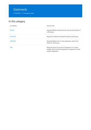
![DEFINE
11/30/2021 • 2 minutes to read
Syntax
DEFINE { <entity> [<name>] = <expression> }
Arguments
TERM DEFINITION
entity MEASURE, VAR, TABLE, or COLUMN.
name The name of an entity. It cannot be an expression.
expression Any DAX expression that returns a single scalar value. The
expression can use any of the defined entities. The
expression must return a table. If a scalar value is required,
wrap the scalar inside a ROW() function to produce a table.
Remarks
See also
A keyword that defines entities that can be applied to one or more EVALUATE statements of a DAX query.
Entities can be variables, measures, tables, and columns.
Definitions typically precede the EVALUATE statement and are valid for all EVALUATE statements.
Definitions can reference other definitions that appear before or after the current definition.
Definitions exist only for the duration of the query.
DAX queries
ORDER BY
VAR](https://image.slidesharecdn.com/funcoesdax-220812141017-bb6cd4dc/85/Funcoes-DAX-pdf-678-320.jpg)
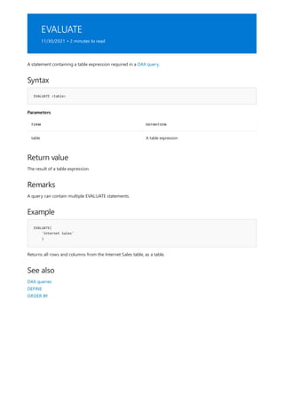
![ORDER BY
11/30/2021 • 2 minutes to read
Syntax
ORDER BY {<expression> [{ASC | DESC}]}
Arguments
TERM DEFINITION
expression Any DAX expression that returns a single scalar value.
ASC (default) Ascending sort order.
DESC Descending sort order.
Return value
Example
EVALUATE(
'Internet Sales'
)
ORDER BY
'Internet Sales'[Order Date]
See also
Defines the sort order of query results returned by an EVALUATE statement in a DAX query.
The result of an EVALUATE statement in ascending (ASC) or descending (DESC) order.
Returns all rows and columns from the Internet Sales table, ordered by Order Date, as a table.
DAX queries
EVALUATE](https://image.slidesharecdn.com/funcoesdax-220812141017-bb6cd4dc/85/Funcoes-DAX-pdf-680-320.jpg)
![VAR
11/30/2021 • 2 minutes to read
Syntax
VAR <name> = <expression>
Parameters
TERM DEFINITION
name The name of the variable (identifier).
Delimiters are not supported. For example, 'varName' or
[varName] will result in an error.
Supported character set: a-z, A-Z, 0-9.
0-9 are not valid as first character.
__ (double underscore) is allowed as a prefix to the identifier
name.
No other special characters are supported.
Reserved keywords not allowed.
Names of existing tables are not allowed.
Empty spaces are not allowed.
expression A DAX expression which returns a scalar or table value.
Return value
Remarks
Example
Stores the result of an expression as a named variable, which can then be passed as an argument to other
measure expressions. Once resultant values have been calculated for a variable expression, those values do not
change, even if the variable is referenced in another expression.
A named variable containing the result of the expression argument.
An expression passed as an argument to VAR can contain another VAR declaration.
When referencing a variable:
Measures cannot refer to variables defined outside the measure expression, but can refer to functional
scope variables defined within the expression.
Variables can refer to measures.
Variables can refer to previously defined variables.
Columns in table variables cannot be referenced via TableName[ColumnName] syntax.
For best practices when using VAR, see Use variables to improve your DAX formulas.
To calculate a percentage of year-over-year growth without using a variable, you could create three separate
measures. This first measure calculates Sum of Sales Amount:](https://image.slidesharecdn.com/funcoesdax-220812141017-bb6cd4dc/85/Funcoes-DAX-pdf-681-320.jpg)
![Sum of SalesAmount = SUM(SalesTable[SalesAmount])
SalesAmount PreviousYear =
CALCULATE([Sum of SalesAmount],
SAMEPERIODLASTYEAR(Calendar[Date])
)
Sum of SalesAmount YoY%: =
IF([Sum of SalesAmount] ,
DIVIDE(([Sum of SalesAmount] – [SalesAmount PreviousYear]), [Sum of SalesAmount])
)
YoY% = VAR Sales = SUM(SalesTable[SalesAmount])
VAR SalesLastYear =
CALCULATE ( SUM ( SalesTable[SalesAmount] ), SAMEPERIODLASTYEAR ( 'Calendar'[Date] ) )
return if(Sales, DIVIDE(Sales – SalesLastYear, Sales))
A second measure calculates the sales amount for the previous year:
You can then create a third measure that combines the other two measures to calculate a growth percentage.
Notice the Sum of SalesAmount measure is used in two places; first to determine if there is a sale, then again to
calculate a percentage.
By using a variable, you can create a single measure that calculates the same result:
By using a variable, you can get the same outcome, but in a more readable way. In addition, the result of the
expression is stored in the variable upon declaration. It doesn't have to be recalculated each time it is used, as it
would without using a variable. This can improve the measure's performance.](https://image.slidesharecdn.com/funcoesdax-220812141017-bb6cd4dc/85/Funcoes-DAX-pdf-682-320.jpg)
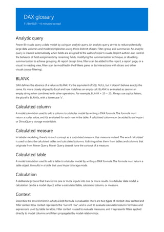
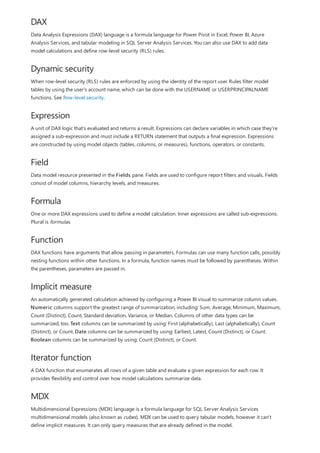
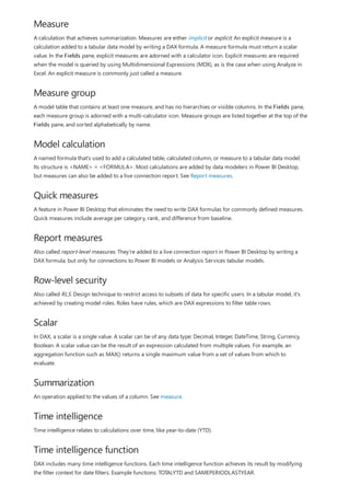
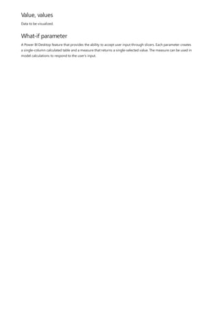
![DAX operators
11/30/2021 • 6 minutes to read
Types of operators
Arithmetic operators
ARITHMETIC OPERATOR MEANING EXAMPLE
+ (plus sign) Addition 3+3
– (minus sign) Subtraction or sign 3–1–1
* (asterisk) Multiplication 3*3
/ (forward slash) Division 3/3
^ (caret) Exponentiation 16^4
NOTE
Comparison operators
COMPARISON OPERATOR MEANING EXAMPLE
= Equal to [Region] = "USA"
== Strict equal to [Region] == "USA"
> Greater than [Sales Date] > "Jan 2009"
< Less than [Sales Date] < "Jan 1 2009"
>= Greater than or equal to [Amount] >= 20000
The Data Analysis Expression (DAX) language uses operators to create expressions that compare values, perform
arithmetic calculations, or work with strings.
There are four different types of calculation operators: arithmetic, comparison, text concatenation, and logical.
To perform basic mathematical operations such as addition, subtraction, or multiplication; combine numbers;
and produce numeric results, use the following arithmetic operators.
The plus sign can function both as a binary operator and as a unary operator. A binary operator requires numbers on
both sides of the operator and performs addition. When you use values in a DAX formula on both sides of the binary
operator, DAX tries to cast the values to numeric data types if they are not already numbers. In contrast, the unary
operator can be applied to any type of argument. The plus symbol does not affect the type or value and is simply ignored,
whereas the minus operator creates a negative value, if applied to a numeric value.
You can compare two values with the following operators. When two values are compared by using these
operators, the result is a logical value, either TRUE or FALSE.](https://image.slidesharecdn.com/funcoesdax-220812141017-bb6cd4dc/85/Funcoes-DAX-pdf-687-320.jpg)
![<= Less than or equal to [Amount] <= 100
<> Not equal to [Region] <> "USA"
COMPARISON OPERATOR MEANING EXAMPLE
Text concatenation operator
TEXT OPERATOR MEANING EXAMPLE
& (ampersand) Connects, or concatenates, two values
to produce one continuous text value
[Region] & ", " & [City]
Logical operators
TEXT OPERATOR MEANING EXAMPLES
&& (double ampersand) Creates an AND condition between
two expressions that each have a
Boolean result. If both expressions
return TRUE, the combination of the
expressions also returns TRUE;
otherwise the combination returns
FALSE.
([Region] = "France") && ([BikeBuyer]
= "yes"))
|| (double pipe symbol) Creates an OR condition between two
logical expressions. If either expression
returns TRUE, the result is TRUE; only
when both expressions are FALSE is
the result FALSE.
(([Region] = "France") || ([BikeBuyer] =
"yes"))
IN Creates a logical OR condition between
each row being compared to a table.
Note: the table constructor syntax uses
curly braces.
'Product'[Color] IN { "Red", "Blue",
"Black" }
Operators and precedence order
Calculation order
Operator precedence
All comparison operators except == treat BLANK as equal to number 0, empty string "", DATE(1899, 12, 30), or
FALSE. As a result, [Column] = 0 will be true when the value of [Column] is either 0 or BLANK. In contrast,
[Column] == 0 is true only when the value of [Column] is 0.
Use the ampersand (&) to join, or concatenate, two or more text strings to produce a single piece of text.
Use logical operators (&&) and (||) to combine expressions to produce a single result.
In some cases, the order in which calculation is performed can affect the Return value; therefore, it is important
to understand how the order is determined and how you can change the order to obtain the desired results.
An expression evaluates the operators and values in a specific order. All expressions always begin with an equal
sign (=). The equal sign indicates that the succeeding characters constitute an expression.
Following the equal sign are the elements to be calculated (the operands), which are separated by calculation
operators. Expressions are always read from left to right, but the order in which the elements are grouped can
be controlled to some degree by using parentheses.](https://image.slidesharecdn.com/funcoesdax-220812141017-bb6cd4dc/85/Funcoes-DAX-pdf-688-320.jpg)
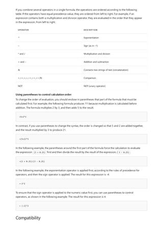
![Coercing data types of operands
LEFT SIDE DATA TYPE RIGHT SIDE DATA TYPE
Numeric Numeric
Boolean Boolean
String String
DATA TYPES USED IN DAX DATA TYPES USED IN EXCEL
Numbers (I8, R8) Numbers (R8)
String String
Boolean Boolean
DateTime Variant
Currency Currency
Differences in precedence order
DAX easily handles and compares various data types, much like Microsoft Excel. However, the underlying
computation engine is based on SQL Server Analysis Services and provides additional advanced features of a
relational data store, including richer support for date and time types. Therefore, in some cases the results of
calculations or the behavior of functions may not be the same as in Excel. Moreover, DAX supports more data
types than does Excel. This section describes the key differences.
In general, the two operands on the left and right sides of any operator should be the same data type. However,
if the data types are different, DAX will convert them to a common data type to apply the operator in some
cases:
1. Both operands are converted to the largest possible common data type.
2. The operator is applied, if possible.
For example, suppose you have two numbers that you want to combine. One number results from a formula,
such as = [Price] * .20 , and the result may contain many decimal places. The other number is an integer that
has been provided as a string value.
In this case, DAX will convert both numbers to real numbers in a numeric format, using the largest numeric
format that can store both kinds of numbers. Then DAX will apply the multiplication.
Depending on the data-type combination, type coercion may not be applied for comparison operations. For a
complete list of data types supported by DAX, see Data types supported in tabular models and Data types in
Power BI Desktop.
Integer, Real Number, Currency, Date/time and Blank are considered numeric for comparison purposes. Blank
evaluates to zero when performing a comparison. The following data-type combinations are supported for
comparison operations.
Other mixed data-type comparisons will return an error. For example, a formula such as ="1" > 0 returns an
error stating that DAX comparison operations do not support comparing values of type Text with values of type
Integer.
The precedence order of operations in DAX formulas is basically the same as that used by Microsoft Excel, but](https://image.slidesharecdn.com/funcoesdax-220812141017-bb6cd4dc/85/Funcoes-DAX-pdf-690-320.jpg)
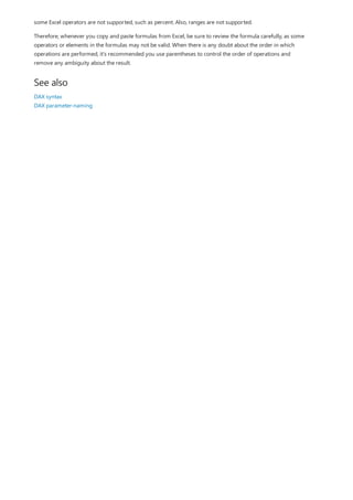
![DAX queries
11/30/2021 • 4 minutes to read
Syntax
[DEFINE { MEASURE <tableName>[<name>] = <expression> }
{ VAR <name> = <expression>}]
EVALUATE <table>
[ORDER BY {<expression> [{ASC | DESC}]}[, …]
[START AT {<value>|<parameter>} [, …]]]
Keywords
EVALUATE (Required)
Syntax
EVALUATE <table>
Arguments
TERM DEFINITION
table A table expression.
Example
EVALUATE(
'Internet Sales'
)
With DAX queries, you can query and return data defined by a table expression. Reporting clients construct DAX
queries whenever a field is placed on a report surface, or a whenever a filter or calculation is applied. DAX
queries can also be created and run in SQL Server Management Studio (SSMS) and open-source tools like DAX
Studio. DAX queries run in SSMS and DAX Studio return results as a table.
Before learning about queries, it's important you have a solid understanding of DAX basics. If you haven't
already, be sure to checkout DAX overview.
At the most basic level, a DAX query is an EVALUATE statement containing a table expression. However, a query
can contain multiple EVALUATE statements.
Returns all rows and columns from the Internet Sales table, as a table.](https://image.slidesharecdn.com/funcoesdax-220812141017-bb6cd4dc/85/Funcoes-DAX-pdf-692-320.jpg)
![ORDER BY (Optional)
Syntax
EVALUATE <table>
[ORDER BY {<expression> [{ASC | DESC}]}[, …]
Arguments
TERM DEFINITION
expression Any DAX expression that returns a single scalar value.
ASC (default) Ascending sort order.
DESC Descending sort order.
Example
EVALUATE(
'Internet Sales'
)
ORDER BY
'Internet Sales'[Order Date]
The optional ORDER BY keyword defines one or more expressions used to sort query results. Any expression
that can be evaluated for each row of the result is valid.
Returns all rows and columns from the Internet Sales table, ordered by Order Date, as a table.](https://image.slidesharecdn.com/funcoesdax-220812141017-bb6cd4dc/85/Funcoes-DAX-pdf-693-320.jpg)
![START AT (Optional)
Syntax
EVALUATE <table>
[ORDER BY {<expression> [{ASC | DESC}]}[, …]
[START AT {<value>|<parameter>} [, …]]]
Arguments
TERM DEFINITION
value A constant value. Cannot be an expression.
parameter The name of a parameter in an XMLA statement prefixed
with an @ character.
Example
EVALUATE(
'Internet Sales'
)
ORDER BY
'Internet Sales'[Sales Order Number]
START AT "SO7000"
The optional START AT keyword is used inside an ORDER BY clause. It defines the value at which the query
results begin.
START AT arguments have a one-to-one correspondence with the columns in the ORDER BY clause. There can be
as many arguments in the START AT clause as there are in the ORDER BY clause, but not more. The first
argument in the START AT defines the starting value in column 1 of the ORDER BY columns. The second
argument in the START AT defines the starting value in column 2 of the ORDER BY columns within the rows that
meet the first value for column 1.
Returns all rows and columns from the Internet Sales table, ordered by Sales Order Number, beginning at
SO7000.](https://image.slidesharecdn.com/funcoesdax-220812141017-bb6cd4dc/85/Funcoes-DAX-pdf-694-320.jpg)
![DEFINE (Optional)
Syntax
[DEFINE { MEASURE <tableName>[<name>] = <expression> }
{ VAR <name> = <expression>}]
EVALUATE <table>
Arguments
TERM DEFINITION
tableName The name of an existing table using standard DAX syntax. It
cannot be an expression.
name The name of a new measure. It cannot be an expression.
expression Any DAX expression that returns a single scalar value. The
expression can use any of the defined measures. The
expression must return a table. If a scalar value is required,
wrap the scalar inside a ROW() function to produce a table.
VAR An optional expression as a named variable. A VAR can be
passed as an argument to other expressions.
Example
Multiple EVALUATE/ORDER BY/START AT clauses can be specified in a single query.
The optional DEFINE keyword defines entities that exist only for the duration of the query. Definitions are valid
for all EVALUATE statements. Entities can be variables, measures, tables, and columns. Definitions can reference
other definitions that appear before or after the current definition. Definitions typically precede the EVALUATE
statement.](https://image.slidesharecdn.com/funcoesdax-220812141017-bb6cd4dc/85/Funcoes-DAX-pdf-695-320.jpg)
![DEFINE
MEASURE 'Internet Sales'[Internet Total Sales] = SUM('Internet Sales'[Sales Amount])
EVALUATE
SUMMARIZECOLUMNS
(
'Date'[Calendar Year],
TREATAS({2013, 2014}, 'Date'[Calendar Year]),
"Total Sales", [Internet Total Sales],
"Combined Years Total Sales", CALCULATE([Internet Total Sales], ALLSELECTED('Date'[Calendar Year]))
)
ORDER BY [Calendar Year]
Parameters in DAX queries
IMPORTANT
See also
Returns the calculated total sales for years 2013 and 2014, and combined calculated total sales for years 2013
and 2014, as a table. The measure in the DEFINE statement, Internet Total Sales, is used in both Total Sales and
Combined Years Total Sales expressions.
A well-defined DAX query statement can be parameterized and then used over and over with just changes in the
parameter values.
The Execute Method (XMLA) method has a Parameters Element (XMLA) collection element that allows
parameters to be defined and assigned a value. Within the collection, each Parameter Element (XMLA) element
defines the name of the parameter and a value to it.
Reference XMLA parameters by prefixing the name of the parameter with an @ character. Any place in the
syntax where a value is allowed, the value can be replaced with a parameter call. All XMLA parameters are typed
as text.
Parameters defined in the parameters section and not used in the <STATEMENT> element generate an error response in
XMLA. Parameters used and not defined in the <Parameters> element generate an error response in XMLA.
FILTER](https://image.slidesharecdn.com/funcoesdax-220812141017-bb6cd4dc/85/Funcoes-DAX-pdf-696-320.jpg)

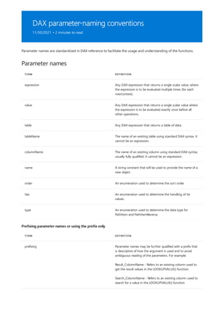
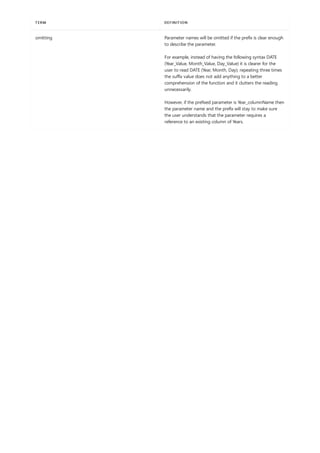
![DAX syntax
11/30/2021 • 9 minutes to read
Syntax requirements
FORMULA RESULT
= 3 3
= "Sales" Sales
= 'Sales'[Amount] If you use this formula within the Sales table, you will get the
value of the column Amount in the Sales table for the
current row.
= (0.03 *[Amount])
=0.03 * [Amount]
Three percent of the value in the Amount column of the
current table.
Although this formula can be used to calculate a percentage,
the result is not shown as a percentage unless you apply
formatting in the table.
= PI() The value of the constant pi.
This article describes syntax and requirements for the DAX formula expression language.
A DAX formula always starts with an equal sign (=). After the equals sign, you can provide any expression that
evaluates to a scalar, or an expression that can be converted to a scalar. These include the following:
A scalar constant, or expression that uses a scalar operator (+,-,*,/,>=,...,&&, ...)
References to columns or tables. The DAX language always uses tables and columns as inputs to
functions, never an array or arbitrary set of values.
Operators, constants, and values provided as part of an expression.
The result of a function and its required arguments. Some DAX functions return a table instead of a scalar,
and must be wrapped in a function that evaluates the table and returns a scalar; unless the table is a
single column, single row table, then it is treated as a scalar value.
Most DAX functions require one or more arguments, which can include tables, columns, expressions, and
values. However, some functions, such as PI, do not require any arguments, but always require
parentheses to indicate the null argument. For example, you must always type PI(), not PI. You can also
nest functions within other functions.
Expressions. An expression can contain any or all of the following: operators, constants, or references to
columns.
For example, the following are all valid formulas.
Formulas can behave differently depending on how they are used. You must always be aware of the context and
how the data that you use in the formula is related to other data that might be used in the calculation.](https://image.slidesharecdn.com/funcoesdax-220812141017-bb6cd4dc/85/Funcoes-DAX-pdf-700-320.jpg)
![Naming requirements
NOTE
Tables
Measures
Columns
A data model often contains multiple tables. Together the tables and their columns comprise a database stored
in the in-memory analytics engine (VertiPaq). Within that database, all tables must have unique names. The
names of columns must also be unique within each table. All object names are case-insensitive; for example, the
names SALES and Sales would represent the same table.
Each column and measure you add to an existing data model must belong to a specific table. You specify the
table that contains the column either implicitly, when you create a calculated column within a table, or explicitly,
when you create a measure and specify the name of the table where the measure definition should be stored.
When you use a table or column as an input to a function, you must generally qualify the column name. The
fully qualified name of a column is the table name, followed by the column name in square brackets: for
examples, 'U.S. Sales'[Products]. A fully qualified name is always required when you reference a column in the
following contexts:
As an argument to the function, VALUES
As an argument to the functions, ALL or ALLEXCEPT
In a filter argument for the functions, CALCULATE or CALCULATETABLE
As an argument to the function, RELATEDTABLE
As an argument to any time intelligence function
An unqualified column name is just the name of the column, enclosed in brackets: for example, [Sales Amount].
For example, when you are referencing a scalar value from the same row of the current table, you can use the
unqualified column name.
If the name of a table contains spaces, reserved keywords, or disallowed characters, you must enclose the table
name in single quotation marks. You must also enclose table names in quotation marks if the name contains any
characters outside the ANSI alphanumeric character range, regardless of whether your locale supports the
character set or not. For example, if you open a workbook that contains table names written in Cyrillic
characters, such as 'Таблица', the table name must be enclosed in quotation marks, even though it does not
contain spaces.
To make it easier to enter the fully qualified names of columns, use the AutoComplete feature in the formula editor.
Table names are required whenever the column is from a different table than the current table. Table
names must be unique within the database.
Table names must be enclosed in single quotation marks if they contain spaces, other special characters
or any non-English alphanumeric characters.
Measure names must always be in brackets.
Measure names can contain spaces.
Each measure name must be unique within a model. Therefore, the table name is optional in front of a
measure name when referencing an existing measure. However, when you create a measure you must
always specify a table where the measure definition will be stored.](https://image.slidesharecdn.com/funcoesdax-220812141017-bb6cd4dc/85/Funcoes-DAX-pdf-701-320.jpg)
![Reserved keywords
NOTE
Special characters
Examples of object names
OBJECT TYPES EXAMPLES COMMENT
Table name Sales If the table name does not contain
spaces or other special characters, the
name does not need to be enclosed in
quotation marks.
Table name 'Canada Sales' If the name contains spaces, tabs or
other special characters, enclose the
name in single quotation marks.
Fully qualified column name Sales[Amount] The table name precedes the column
name, and the column name is
enclosed in brackets.
Fully qualified measure name Sales[Profit] The table name precedes the measure
name, and the measure name is
enclosed in brackets. In certain
contexts, a fully qualified name is
always required.
Column names must be unique in the context of a table; however, multiple tables can have columns with the
same names (disambiguation comes with the table name).
In general, columns can be referenced without referencing the base table that they belong to, except when there
might be a name conflict to resolve or with certain functions that require column names to be fully qualified.
If the name that you use for a table is the same as an Analysis Services reserved keyword, an error is raised, and
you must rename the table. However, you can use keywords in object names if the object name is enclosed in
brackets (for columns) or quotation marks (for tables).
Quotation marks can be represented by several different characters, depending on the application. If you paste formulas
from an external document or Web page, make sure to check the ASCII code of the character that is used for opening and
closing quotes, to ensure that they are the same. Otherwise DAX may be unable to recognize the symbols as quotation
marks, making the reference invalid.
The following characters and character types are not valid in the names of tables, columns, or measures:
Leading or trailing spaces; unless the spaces are enclosed by name delimiters, brackets, or single
apostrophes.
Control characters
The following characters that are not valid in the names of objects:
.,;':/*|?&%$!+=()[]{}<>
The following table shows examples of some object names:](https://image.slidesharecdn.com/funcoesdax-220812141017-bb6cd4dc/85/Funcoes-DAX-pdf-702-320.jpg)
![Unqualified column name [Amount] The unqualified name is just the
column name, in brackets. Contexts
where you can use the unqualified
name include formulas in a calculated
column within the same table, or in an
aggregation function that is scanning
over the same table.
Fully qualified column in table with
spaces
'Canada Sales'[Qty] The table name contains spaces, so it
must be surrounded by single quotes.
OBJECT TYPES EXAMPLES COMMENT
Other restrictions
DAX operators and constants
OPERATOR TYPE SYMBOL AND USE
Parenthesis operator () precedence order and grouping of arguments
Arithmetic operators + (addition)
- (subtraction/
sign)
* (multiplication)
/ (division)
^ (exponentiation)
Comparison operators = (equal to)
> (greater than)
< (less than)
>= (greater than or equal to)
<= (less than or equal to)
<> (not equal to)
The syntax required for each function, and the type of operation it can perform, varies greatly depending on the
function. In general, however, the following rules apply to all formulas and expressions:
DAX formulas and expressions cannot modify or insert individual values in tables.
You cannot create calculated rows by using DAX. You can create only calculated columns and measures.
When defining calculated columns, you can nest functions to any level.
DAX has several functions that return a table. Typically, you use the values returned by these functions as
input to other functions, which require a table as input.
The following table lists the operators that are supported by DAX. For more information about the syntax of
individual operators, see DAX operators.](https://image.slidesharecdn.com/funcoesdax-220812141017-bb6cd4dc/85/Funcoes-DAX-pdf-703-320.jpg)
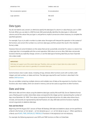
![EVALUATE
FILTER (
FactInternetSales,
[OrderDate] > (DATE(2015,1,9) + TIME(2,30,0)) &&[OrderDate] < (DATE(2015,12,31) + TIME(11,59,59))
)
EVALUATE
FILTER (
FactInternetSales,
[OrderDate] > dt"2015-1-9T02:30:00" && [OrderDate] < dt"2015-12-31T11:59:59"
)
NOTE
The same filter expression can be specified as a literal:
The DAX date and datetime-typed literal format is not supported in all versions of Power BI Desktop, Analysis Services,
and Power Pivot in Excel. New and updated DAX functionality are typically first introduced in Power BI Desktop and then
later included in Analysis Services and Power Pivot in Excel.](https://image.slidesharecdn.com/funcoesdax-220812141017-bb6cd4dc/85/Funcoes-DAX-pdf-705-320.jpg)

This document provides an overview of Data Analysis Expressions (DAX), including how to use DAX formulas to create measures, calculated columns, calculated tables, and row-level security. It describes common DAX functions and concepts like measures, queries, and formula basics. Key information includes how measures dynamically calculate based on filter context, how calculated columns immediately populate column values, and how DAX queries can be used to filter and order data.


