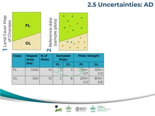
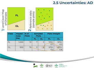
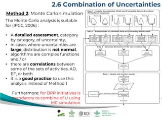
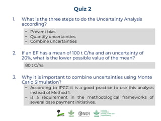
The document discusses uncertainty estimates in greenhouse gas (GHG) inventories as guided by IPCC guidelines, emphasizing the importance of quantifying uncertainties in the FREL (Forest Reference Emission Level). It outlines methods for uncertainty analysis, including Monte Carlo simulation and error propagation, while highlighting criteria for acceptable uncertainty levels across various payment initiatives. Main concepts include the need for transparency, accuracy, and bias prevention in data collection and emissions estimates.

2. Sessions 5 and 6
FREL Uncertainties Estimates
Oswaldo Carrillo
15 April 2020

3. Outline
1. Context
2. IPCC Uncertainties Concepts
3. Running Monte Carlo
simulation
2
Quiz

4. 1. Context

5. The Annex to decision 12 / CP.17 establishes that the
information established in the FREL should be guided by
the most recent IPCC guidelines.
According to IPCC (2006), uncertainty
estimates are an essential element of a
complete GHG inventory.
Emissions/removals estimates are based on:
(1) conceptualization,
(2) models and
(3) input data and assumptions.
Each of these three can be a source of
uncertainty
1. Context

6. Lack of knowledge of the true value
of a variable that can be described as a
probability density function (PDF)
characterising the range and likelihood
of possible values (IPCC, 2006).
What does Uncertainties is?
What does Combination of Uncertainties is?
Once the uncertainties in AD, EF or emissions
for a category have been determined, they may
be combined to provide uncertainty estimates
for the entire inventory (IPCC, 2006)
1. Context
EF
100 t C/ha
30%
of U
(70 t C/ha - 130 t C/ha)

7. It is good practice to account, as far as
possible, for all causes of U (IPCC, 2006)
Why it is important to Quantify the U of the FREL?
What is the acceptable U for the FREL ?
Quantification of U in the FREL is a requirement
in the methodological frameworks of several base
payment initiatives:
REDD Early
Movers
Programme
Same as FCPF and
BCF but different
Reversal Buffer
No
threshold
for
UNFCCC
Criteria Score
If U > 50% 0
30>U<=50% 1
If U >= 30% 2
Criteria Reversal Buffer
≤ 15% 0%
> 15% and ≤ 30% 4%
> 30% and ≤ 60% 8%
> 60% and ≤ 100% 12%
> 100% 15%

8. Quiz 1
1. Why it is important to quantify uncertainties of the FREL?
2. Why does we need to quantify uncertainties of the FREL
using IPCC guidelines?
3. What is the acceptable uncertainty for the FREL
according to Green Climate Found?
• It is good practice to account, as far as possible, for all causes
of U (IPCC, 2006)
• is a requirement in the methodological frameworks of
several base payment initiatives
The Annex to decision 12/CP.17 establishes that the information
established in the FREL should be guided by the most recent
IPCC guidelines.
Ideally <= 30%

9. 2. IPCC Uncertainties
Concepts

10. The Annex to decision 12 / CP.17 establishes that
the information established in the FREL should
be guided by the most recent IPCC guidelines
and be:
• transparent,
• consistent,
• comparable,
• complete and,
• accurate.
• Accuracy means that emission and
removal estimates should be
accurate in the sense that they are
systematically neither over nor
under true emissions or removals,
as far as can be judged, and
• that uncertainties are reduced as
far as practicable.
• Appropriate methodologies should
be used, in accordance with the
2006 IPCC Guidelines (decision 12 /
CP.17)
2. IPCC Uncertainties
Concepts

11. 2.2 Basis for Uncertainty Analysis (IPCC, 2006):
The estimation of
emissions should
prevent bias
(avoiding incorrect
conceptualizations,
models, inputs and
assumptions)
Once biases are
corrected, to the
extent possible, the
uncertainty
analysis can then
focus on
quantification of
the random errors
with respect to the
mean estimate
Once the
uncertainties of the
different sources for a
category have been
correctly determined,
they can be combined
to obtain the
uncertainties of the
emissions. There are
two methods:
• Method 1 uses IPCC
equations,
• Method 2 uses the
Monte Carlo
technique
Prevent bias Quantification of U Combination of U1. 2. 3.

12. Accuracy: Agreement between the true value and the
average of repeated estimates of a variable
Precision: Agreement among repeated
measurements of the same variable. Better
precision means less random error. Precision is
independent of accuracy
2.3 Basic Terminology
Bias: Lack of accuracy

13. 2.4 Bias
Bias can occur because of :
• imperfections in conceptualisation, models, measurement techniques,
• failure to capture all relevant processes involved or
• the available data are not representative of all real-world situations, or
• of instrument error.
Examples of bias in AD
To estimate de AD and prevent bias, it is
necessary to estimate unbiased areas
using reference data (sample plots)
To prevent bias in EF it necessary to
use the right statistical estimator
according to the sampling design
of the NFI
!R! =
∑"#$
%!
y"!
∑"#$
%!
𝑎&'
̅𝑥(´ = *
̅𝑥" 𝑤"(
𝑤
• Simple average
• Ratio estimator
• Weighted estimator
Examples of bias in EF
Mapped AD
(Bias AD)
Mapped AD +Accuracy A.
(Unbiased AD)
Bias in AD
̅𝑥 = *
𝑥"
𝑛

14. 2.5 Uncertainties: concepts
Uncertainty:
Lack of knowledge of the true value of a variable
that can be described as a probability density
function (PDF) characterising the range and
likelihood of possible values.
Causes of U:
• Lack of
completeness
• Lack of data
• Lack of
representativen
ess of data
• Statistical
random
sampling error
• Measurement
error
• Missing data
Symmetric uncertainty
of ±30% relative to the
mean
Asymmetric uncertainty
of -50% to +100% relative
to the mean

15. 2.5 Uncertainties: AD
According to Chapter 3 of Vol. 4 of 2006 IPCC Guidelines:
• Uncertainties associated with the approaches used to
representing land use area should be quantified and reduced as
far as practicable
• Land-use area uncertainty estimates are required as an input to
overall uncertainty analysis
• In Approach 3 “SPATIALLY-EXPLICIT LAND-USE CONVERSION
DATA” the amount of uncertainty can be estimated more
accurately because errors are mapped and can be tested
against independent data/field checked

16. 2.5 Uncertainties: ADLandCoverMap
ofChanges
1
GL
FL

17. 2.5 Uncertainties: ADLandCoverMap
ofChanges
1
GL
FL
Referencedata
(sampleplots)
2

18. 2.5 Uncertainties: ADLandCoverMap
ofChanges
1
GL
FL
Referencedata
(sampleplots)
2

19. 2.5 Uncertainties: ADLandCoverMap
ofChanges
1
GL
FL
Referencedata
(sampleplots)
2

20. 2.5 Uncertainties: ADLandCoverMap
ofChanges
1
GL
FL
Referencedata
(sampleplots)
2

21. 2.5 Uncertainties: ADLandCoverMap
ofChanges
1
GL
FL
Referencedata
(sampleplots)
2

22. 2.5 Uncertainties: ADLandCoverMap
ofChanges
1
GL
FL
Referencedata
(sampleplots)
2

23. 2.5 Uncertainties: ADLandCoverMap
ofChanges
1
GL
FL
Referencedata
(sampleplots)
Estimationsof
unbiasedADanditsU
1) Estimations of weight:
W!
"
n!!
n!.
1 −
n!!
n!.
n!. − 1
2) Estimation of unbiased AD:
3) Estimation of SE of unbiased AD:
S 'A$ = A%&%×S +p.$
S +p.$ = ∑'(!
)
W'
"
!"#
!".
!*
!"#
!".
+".*!
2
3

24. 2.5 Uncertainties: ADLandCoverMap
ofChanges
1
GL
FL
Referencedata
(sampleplots)
Estimationsof
unbiasedADanditsU
1) Estimations of weight:
W!
"
n!!
n!.
1 −
n!!
n!.
n!. − 1
2) Estimation of unbiased AD:
3) Estimation of SE of unbiased AD:
S 'A$ = A%&%×S +p.$
S +p.$ = ∑'(!
)
W'
"
!"#
!".
!*
!"#
!".
+".*!
2
3

25. 2.5 Uncertainties: ADLandCoverMap
ofChanges
1
GL
FL
Referencedata
(sampleplots)
Estimationsof
unbiasedADanditsU
1) Estimations of weight:
W!
"
n!!
n!.
1 −
n!!
n!.
n!. − 1
2) Estimation of unbiased AD:
3) Estimation of SE of unbiased AD:
S 'A$ = A%&%×S +p.$
S +p.$ = ∑'(!
)
W'
"
!"#
!".
!*
!"#
!".
+".*!
2
3

26. 2.5 Uncertainties: ADLandCoverMap
ofChanges
1
GL
FL
Referencedata
(sampleplots)
Estimationsof
unbiasedADanditsU
1) Estimations of weight:
W!
"
n!!
n!.
1 −
n!!
n!.
n!. − 1
2) Estimation of unbiased AD:
3) Estimation of SE of unbiased AD:
S 'A$ = A%&%×S +p.$
S +p.$ = ∑'(!
)
W'
"
!"#
!".
!*
!"#
!".
+".*!
2
3

27. The are several paper where the estimation of unbiased
estimators of AD and its uncertainties is explained
2.5 Uncertainties: AD

28. According to Chave, there are several sources of
uncertainties in the estimations of EF
2.5 Uncertainties: EF

29. According to Chave,
there are several
sources of uncertainties
in the estimations of EF
DBH=30cm
U= 10%
IC: 27-33
Random DBH=32
Bimass (30 cm)=100 kg
U=40%
IC: 60-140
Random Biomass: 130
Measurement
error
Model error
Confidence Interval
2.5 Uncertainties: EF

30. 2.6 Combination of Uncertainties
Once the uncertainties of the different sources for a category have been
correctly determined, they can be combined to obtain the uncertainties of
the emissions.
According to the IPCC (2006), there are two methods to combine them:
Method 1 uses simple error propagation equations, while Method 2 uses
the Monte Carlo technique or similar
Class/Com
ponent
Emission
Factor
Uncertainty
of EF (UEF)
AD
Uncertainty
of AD (UAD)
Emission
(at component level)
Uncertainty of E (UE)
A EF1A UEF1A AD1A UAD1A E1A=EF1A*AD1A
B EF1B UEF1B AD1B UAD1B E1B=EF1B*AD1B
C EF1C UEF1C AD1C UADF1C E1C=EF1C*AD1C
E1=E1A+E1B+E1C
Total emission / Propagated uncertainty of
Transition 1
Transition 1 (FL-OU)
𝑈"#$ = 𝑈"&#$
'
+ 𝑈$)#$
'
𝑈"#* = 𝑈"&#*
'
+ 𝑈$)#*
'
𝑈"#+ = 𝑈"&#+
'
+ 𝑈$)#+
'
𝑈"# =
("-.×01-.)34("-5×01-5)34("-6×01-6)3
"-.4"-54"-6
Method 1: simple error propagation equations

31. The Monte Carlo analysis is suitable
for (IPCC, 2006) :
• A detailed assessment, category
by category, of uncertainty,
• in cases where uncertainties are
large, distribution is not normal,
• algorithms are complex functions
and / or
• there are correlations between
some of the sets of activities, AD,
EF, or both
• it is a good practice to use this
analysis instead of Method 1
Furthermore: for BPR initiatives is
mandatory to combine of U using
MC simulation
2.6 Combination of Uncertainties
Method 2: Monte Carlo simulation

32. Quiz 2
1. What is the three steps to do the Uncertainty Analysis
according?
2. If an EF has a mean of 100 t C/ha and an uncertainty of
20%, what is the lower possible value of the mean?
3. Why it is important to combine uncertainties using Monte
Carlo Simulation?
• Prevent bias
• Quantify uncertainties
• Combine uncertainties
80 t C/ha
• According to IPCC it is a good practice to use this analysis
instead of Method 1.
• is a requirement in the methodological frameworks of
several base payment initiatives.

33. 3. Running Monte
Carlo simulation

34. 3.1 Example of M1:Inputs:
• AD and EF from FOLU sector of the Indonesia 2nd BUR
• Uncerntanties of AD and EF from de FREL 2016
Example of combining uncertainties using Method 1 in
Sumatera for the period 2016-2017
M1 is valid to apply only when:
• Sd/mean<0.3 (small Uncertainties)
• Symmetric distributions
• Inputs are uncorrelated
Class AD
(Ha)
U of
AD
EF
(t CO2e/Ha)
U of
EF
Emissions
(t CO2e)
U of
Emissions
(Emissions x UEmissions)2
Primary dry land
forest
14,647 12 % 463 3 % 6,786,224 (122+32)1/2=
12 %
(6,786,224 x 12)2=
7.16E+15
Secondary dry
land forest
93,599 12 % 314 4 % 29,415,945 (122+42)1/2=
13 %
(29,415,945 x 13)2=
1.36E+17
Primary
mangrove forest
1,182 12 % 455 9 % 538,101 (122+92)1/2=
15 %
(538,101 x 15)2=
6.53E+13
Primary swamp
forest
893 12 % 381 11 % 340,294 (122+112)1/2=
16 %
(340,294 x 16)2=
3.02E+13
Secondary
mangrove forest
8,214 12 % 348 12 % 2,858,136 (122+122)1/2=
17 %
(2,858,136 x 17)2=
1.78E+15
Secondary
swamp forest
39,001 12 % 261 5 % 10,185,146 (122+52)1/2=
13 %
(10,185,146 x 13)2=
7.16E+16
Sum of
Emissions
U of Total
Emissions
Som of
(Emissions x UEmissions)2
50,123,846 405,085,514
/50,123,846 =
8 %
(7.16E+15 + 1.36E + 6.53E+13 +
3.02E+13 + 1.78E+15 + 7.16E+16)1/2=
405,085,514

35. 3.2 Example of Monte Carlo simulation: Multiplication
1,040ha 1,323ha
2.5th
percentile
97.5th
percentile
-12% +12%
1,182ha
Red area acumulate 95% of the probability
414 496
2.5th
percentile
97.5th
percentile
-9% +9%
455
Red area acumulate 95% of the probability
Random Number
Normal DistributionAD
ID iterate AD Simulated EF Simulated Emision Simulated
Random Number
Normal DistributionEF
AD EF

36. 1,040ha 1,323ha1,2311,182ha
414 496455
ID iterate AD Simulated EF Simulated Emision Simulated
1,2311 428 526, 421
Random Number
Normal DistributionAD Random Number
Normal DistributionEF
428
3.2 Example of Monte Carlo simulation: Multiplication
AD EF

37. 1,040ha 1,323ha1,2311,182ha
414 496455
ID iterate AD Simulated EF Simulated Emision Simulated
1,2311 428 526, 421
Random Number
Normal DistributionAD Random Number
Normal DistributionEF
428 454
1,169
1,1692 454 531, 019
3.2 Example of Monte Carlo simulation: Multiplication
AD EF

38. 1,040ha 1,323ha1,084 1,182ha
414 496455
ID iterate AD Simulated EF Simulated Emision Simulated
1,2311 428 526, 421
Random Number
Normal DistributionAD Random Number
Normal DistributionEF
450454
1,169
1,1692 454 531, 019
1,0843 450 488, 053
3.2 Example of Monte Carlo simulation: Multiplication
AD EF

39. 1,040ha 1,323ha1,084 1,182ha
414 496455
ID iterate AD Simulated EF Simulated Emision Simulated
1,2311 428 526, 421
Random Number
Normal DistributionAD Random Number
Normal DistributionEF
450
1,1692 454 531, 019
1,0843 450 488, 053
4
5
6
7
8
9
10
.
.
...
.
...
.
...
1,23110,000 433 532, 413
.
...
1,231
433
3.2 Example of Monte Carlo simulation: Multiplication
AD EF

40. 1,040ha 1,323ha1,182ha
414 496455
Random Number
Normal DistributionAD Random Number
Normal DistributionEF
ID iterate AD Simulated EF Simulated Emision Simulated
1,2311 428 526, 421
1,1692 454 531, 019
1,0843 450 488, 053
4
5
6
7
8
9
10
.
.
...
.
...
.
...
1,23110,000 433 532, 413
.
...
3.2 Example of Monte Carlo simulation: Multiplication
AD EF

41. 1,040ha 1,323ha1,182ha
414 496455
ID iterate AD Simulated EF Simulated Emision Simulated
1,2311 428 526, 421
1,1692 454 531, 019
1,0843 450 488, 053
4
5
6
7
8
9
10
.
.
...
.
...
.
...
1,23110,000 433 532, 413
.
...
3.2 Example of Monte Carlo simulation: Multiplication
AD EF
Percentile2.5%
619,971
Percentile97.5%
460,416
Average:
537,788
CI = Per 97.5-Per 2.5
CI = 460,416 - 619,971 = 159,556
U= ((0.5 x IC)/Average) x 100
U= ((0.5 x 159,556)/537,788) x 100
U= 15%

42. 3.2 Example of Monte Carlo simulation: Sum
AD EF
14,647 463
12 3
AD EF
93,599 314
12 4
AD EF
1,182 455
12 9
AD EF
893 381
12 11
AD EF
8,214 348
12 12
AD EF
39,001 261
12 5
Mean
Uncertainty (%)
ID
iterate
Primary dry
land forest
Secondary dry
land forest
Primary mangrove
forest
Primary swamp
forest
Secondary mangrove
forest
Secondary swamp
forest
Primary dry land
forest
Secondary dry land
forest
Primary mangrove
forest
Primary swamp
forest
Secondary
mangrove forest
Secondary swamp
forest
AD
sim
EF
sim
EM
AD
sim
EF
sim
EM
AD
sim
EF
sim
EM
AD
sim
EF
sim
EM
AD
sim
EF
sim
EM
AD
sim
EF
sim
EM
TOTAL
EMISSION
13,655 4751 104,488 311 1,231 428 808 347 8,279 331 36,539 268
13,655 475 104,488 311 1,231 428 808 347 8,279 331 36,539 268
6.480 32.487 0.526 0.280 2.744 9.800 52.317

43. AD EF
14,647 463
12 3
AD EF
93,599 314
12 4
AD EF
1,182 455
12 9
AD EF
893 381
12 11
AD EF
8,214 348
12 12
AD EF
39,001 261
12 5
Mean
Uncertainty (%)
ID
iterate
Primary dry
land forest
Secondary dry
land forest
Primary mangrove
forest
Primary swamp
forest
Secondary mangrove
forest
Secondary swamp
forest
Primary dry land
forest
Secondary dry land
forest
Primary mangrove
forest
Primary swamp
forest
Secondary
mangrove forest
Secondary swamp
forest
AD
sim
EF
sim
EM
AD
sim
EF
sim
EM
AD
sim
EF
sim
EM
AD
sim
EF
sim
EM
AD
sim
EF
sim
EM
AD
sim
EF
sim
EM
TOTAL
EMISSION
13,655 4751 104,488 311 1,231 428 808 347 8,279 331 36,539 268
13,655 475 104,488 311 1,231 428 808 347 8,279 331 36,539 268
32.487 0.526 0.280 2.744 9.800 52.3176.480
3.2 Example of Monte Carlo simulation: Sum

44. AD EF
14,647 463
12 3
AD EF
93,599 314
12 4
AD EF
1,182 455
12 9
AD EF
893 381
12 11
AD EF
8,214 348
12 12
AD EF
39,001 261
12 5
Mean
Uncertainty (%)
ID
iterate
Primary dry
land forest
Secondary dry
land forest
Primary mangrove
forest
Primary swamp
forest
Secondary mangrove
forest
Secondary swamp
forest
Primary dry land
forest
Secondary dry land
forest
Primary mangrove
forest
Primary swamp
forest
Secondary
mangrove forest
Secondary swamp
forest
AD
sim
EF
sim
EM
AD
sim
EF
sim
EM
AD
sim
EF
sim
EM
AD
sim
EF
sim
EM
AD
sim
EF
sim
EM
AD
sim
EF
sim
EM
TOTAL
EMISSION
13,655 4751 104,488 311 1,231 428 808 347 8,279 331 36,539 26832.487 0.526 0.280 2.744 9.800 52.3176.480
13,698 4672 94,076 314 1,169 454 818 404 7,810 342 38,382 26129.584 0.531 0.330 2.674 10.008 49.5276.400
13,698 467 94,076 314 1,169 454 818 404 7,810 342 38,382 261
3.2 Example of Monte Carlo simulation: Sum

45. AD EF
14,647 463
12 3
AD EF
93,599 314
12 4
AD EF
1,182 455
12 9
AD EF
893 381
12 11
AD EF
8,214 348
12 12
AD EF
39,001 261
12 5
Mean
Uncertainty (%)
ID
iterate
Primary dry
land forest
Secondary dry
land forest
Primary mangrove
forest
Primary swamp
forest
Secondary mangrove
forest
Secondary swamp
forest
Primary dry land
forest
Secondary dry land
forest
Primary mangrove
forest
Primary swamp
forest
Secondary
mangrove forest
Secondary swamp
forest
AD
sim
EF
sim
EM
AD
sim
EF
sim
EM
AD
sim
EF
sim
EM
AD
sim
EF
sim
EM
AD
sim
EF
sim
EM
AD
sim
EF
sim
EM
TOTAL
EMISSION
13,655 4751 104,488 311 1,231 428 808 347 8,279 331 36,539 26832.487 0.526 0.280 2.744 9.800 52.3176.480
13,698 467 94,076 314 1,169 454 818 404 7,810 342 38,382 26129.584 0.531 0.330 2.674 10.008 49.5276.400
13,864 461 95,622 311 1,084 450 808 388 8,181 345 40,896 264
13,864 4613 95,622 311 1,084 450 808 388 8,181 345 40,896 26429.713 0.488 0.313 2.822 10.810 50.5366.390
2
3.2 Example of Monte Carlo simulation: Sum

46. AD EF
14,647 463
12 3
AD EF
93,599 314
12 4
AD EF
1,182 455
12 9
AD EF
893 381
12 11
AD EF
8,214 348
12 12
AD EF
39,001 261
12 5
Mean
Uncertainty (%)
ID
iterate
Primary dry
land forest
Secondary dry
land forest
Primary mangrove
forest
Primary swamp
forest
Secondary mangrove
forest
Secondary swamp
forest
Primary dry land
forest
Secondary dry land
forest
Primary mangrove
forest
Primary swamp
forest
Secondary
mangrove forest
Secondary swamp
forest
AD
sim
EF
sim
EM
AD
sim
EF
sim
EM
AD
sim
EF
sim
EM
AD
sim
EF
sim
EM
AD
sim
EF
sim
EM
AD
sim
EF
sim
EM
TOTAL
EMISSION
13,655 4751 104,488 311 1,231 428 808 347 8,279 331 36,539 26832.487 0.526 0.280 2.744 9.800 52.3176.480
13,698 467 94,076 314 1,169 454 818 404 7,810 342 38,382 26129.584 0.531 0.330 2.674 10.008 49.5276.400
13,864 461 95,622 311 1,084 450 808 388 8,181 345 40,896 264
13,864 461 95,622 311 1,084 450 808 388 8,181 345 40,896 26429.713 0.488 0.313 2.822 10.810 50.5366.390
2
3
.
..
.
..
.
.
.
.
..
.
..
.
.
.
.
..
.
..
.
..
.
..
.
..
.
..
.
..
.
..
.
..
.
..
.
.
.
.
..
.
..
.
..
3.2 Example of Monte Carlo simulation: Sum

47. AD EF
14,647 463
12 3
AD EF
93,599 314
12 4
AD EF
1,182 455
12 9
AD EF
893 381
12 11
AD EF
8,214 348
12 12
AD EF
39,001 261
12 5
Mean
Uncertainty (%)
ID
iterate
Primary dry
land forest
Secondary dry
land forest
Primary mangrove
forest
Primary swamp
forest
Secondary mangrove
forest
Secondary swamp
forest
Primary dry land
forest
Secondary dry land
forest
Primary mangrove
forest
Primary swamp
forest
Secondary
mangrove forest
Secondary swamp
forest
AD
sim
EF
sim
EM
AD
sim
EF
sim
EM
AD
sim
EF
sim
EM
AD
sim
EF
sim
EM
AD
sim
EF
sim
EM
AD
sim
EF
sim
EM
TOTAL
EMISSION
13,655 4751 104,488 311 1,231 428 808 347 8,279 331 36,539 26832.487 0.526 0.280 2.744 9.800 52.3176.480
13,698 467 94,076 314 1,169 454 818 404 7,810 342 38,382 26129.584 0.531 0.330 2.674 10.008 49.5276.400
15,765 462 104,007 312 1,231 433 882 353 8,328 322 37,370 263
13,864 461 95,622 311 1,084 450 808 388 8,181 345 40,896 26429.713 0.488 0.313 2.822 10.810 50.5366.390
2
3
.
..
.
..
.
.
.
.
..
.
..
.
.
.
.
..
.
..
.
..
.
..
.
..
.
..
.
..
.
..
.
..
.
..
.
.
.
.
..
.
..
.
..
15,765 46210,000 104,007 312 1,231 433 882 353 8,328 322 37,370 26332.449 0.532 0.311 2.685 9.833 53.0947.284
3.2 Example of Monte Carlo simulation: Sum

48. AD EF
14,647 463
12 3
AD EF
93,599 314
12 4
AD EF
1,182 455
12 9
AD EF
893 381
12 11
AD EF
8,214 348
12 12
AD EF
39,001 261
12 5
Mean
Uncertainty (%)
Primary dry land
forest
Secondary dry land
forest
Primary mangrove
forest
Primary swamp
forest
Secondary
mangrove forest
Secondary swamp
forest
15,765 462 104,007 312 1,231 433 882 353 8,328 322 37,370 263
3.2 Example of Monte Carlo simulation: Sum
ID
iterate
Primary dry
land forest
Secondary dry
land forest
Primary mangrove
forest
Primary swamp
forest
Secondary mangrove
forest
Secondary swamp
forest
AD
sim
EF
sim
EM
AD
sim
EF
sim
EM
AD
sim
EF
sim
EM
AD
sim
EF
sim
EM
AD
sim
EF
sim
EM
AD
sim
EF
sim
EM
TOTAL
EMISSION
13,655 4751 104,488 311 1,231 428 808 347 8,279 331 36,539 26832.487 0.526 0.280 2.744 9.800 52.3176.480
13,698 467 94,076 314 1,169 454 818 404 7,810 342 38,382 26129.584 0.531 0.330 2.674 10.008 49.5276.400
13,864 461 95,622 311 1,084 450 808 388 8,181 345 40,896 26429.713 0.488 0.313 2.822 10.810 50.5366.390
2
3
.
..
.
..
.
.
.
.
..
.
..
.
.
.
.
..
.
..
.
..
.
..
.
..
.
..
.
..
.
..
.
..
.
..
.
.
.
.
..
.
..
.
..
15,765 46210,000 104,007 312 1,231 433 882 353 8,328 322 37,370 26332.449 0.532 0.311 2.685 9.833 53.0947.284
Percentile2.5%
46,124,368
Percentile97.5%
54,149,192
Average:
50,133,801
CI = Per 97.5-Per 2.5
CI = 54,149,192 - 46,124,368
CI= 8,024,824
U= ((0.5 x IC)/Average) x 100
U= ((0.5 x 8,024,824)/ 50,133,801) x 100
U= 8%

49. 3.3 Exercise of Monte Carlo simulation in Excel
Island: SUMATERA
AD EF Emision AD EF Emision AD EF Emision AD EF Emision AD EF Emision AD EF Emision
Mean 14,647 463 6,786,224 93,599 314 29,415,945 1,182 455 538,101 893 381 340,294 8,214 348 2,858,136 39,001 261 10,185,146
Uncertaint 12 3 12 4 12 9 12 11 12 12 12 5Estandar
Error 897 8 5731 6 72 21 55 21 503 21 2388 7
Id iteration AD_sim EF_sim Em AD_sim EF_sim Em AD_sim EF_sim Em AD_sim EF_sim Em AD_sim EF_sim Em AD_sim EF_sim Em Total Emission
1 13,655 475 6,479,683 104,488 311 32,486,774 1,231 428 526,421 808 347 280,134 8,279 331 2,744,474 36,539 268 9,799,562 52,317,049
2 13,698 467 6,399,795 94,076 314 29,583,888 1,169 454 531,019 818 404 330,031 7,810 342 2,673,525 38,382 261 10,008,387 49,526,645
3 13,864 461 6,389,703 95,622 311 29,713,230 1,084 450 488,053 808 388 313,403 8,181 345 2,821,723 40,896 264 10,809,957 50,536,070
4 13,553 459 6,215,270 103,578 320 33,189,541 1,057 460 486,347 870 362 314,544 8,220 368 3,022,891 41,177 260 10,705,405 53,933,997
5 14,515 460 6,673,706 98,414 316 31,142,092 1,235 440 543,042 942 383 360,782 8,326 338 2,811,910 39,710 275 10,924,373 52,455,905
6 15,373 466 7,161,781 106,236 308 32,762,483 1,052 448 471,048 919 388 356,203 7,837 323 2,530,006 36,642 260 9,520,570 52,802,090
7 14,811 472 6,993,963 101,177 312 31,582,458 1,304 457 596,023 845 354 299,416 7,390 338 2,500,602 41,567 252 10,474,846 52,447,307
8 17,202 469 8,059,571 94,245 315 29,668,779 1,200 490 587,443 992 393 389,302 8,631 346 2,982,244 38,777 268 10,378,900 52,066,239
9 14,108 474 6,684,096 97,707 310 30,303,952 1,227 460 564,768 894 374 334,549 7,382 347 2,559,731 39,918 257 10,243,045 50,690,142
10 13,546 459 6,212,843 93,400 316 29,469,180 1,087 445 483,798 951 404 384,061 7,583 349 2,645,444 34,182 255 8,716,589 47,911,915
11 14,540 461 6,704,175 92,738 308 28,592,050 1,147 460 528,178 984 366 360,379 8,665 321 2,781,776 42,272 260 11,000,219 49,966,777
12 15,470 446 6,901,663 96,125 324 31,148,206 1,221 472 576,718 912 386 351,706 8,894 324 2,877,568 33,359 263 8,769,157 50,625,018
13 14,633 464 6,793,696 90,904 312 28,386,017 1,264 478 603,516 959 405 387,934 8,635 368 3,178,597 43,944 247 10,867,491 50,217,251
14 15,723 464 7,290,211 82,246 321 26,431,107 1,242 483 600,036 935 339 316,831 7,821 337 2,638,565 38,928 252 9,816,328 47,093,078
15 14,180 476 6,743,780 87,731 314 27,523,516 1,276 448 572,040 869 371 322,576 8,323 367 3,057,861 40,089 255 10,229,124 48,448,897
16 16,109 470 7,566,319 101,971 313 31,917,416 1,293 476 615,349 864 378 327,116 9,065 345 3,127,856 45,599 261 11,900,383 55,454,438
Secondary swamp forestPrimary dry land forest Secondary dry land forest Primary mangrove forest Primary swamp forest Secondary mangrove forest
9997 15,194 452 6,867,781 94,511 314 29,715,307 1,325 415 550,157 950 395 374,711 8,595 354 3,041,622 41,619 267 11,100,501 51,650,078
9998 15,138 465 7,043,898 106,480 319 33,978,925 1,229 440 540,958 1,004 413 414,676 8,224 367 3,016,092 36,208 263 9,526,615 54,521,163
9999 15,798 467 7,371,263 103,826 305 31,627,618 1,238 461 570,394 906 420 380,969 8,359 354 2,956,415 37,469 267 9,988,108 52,894,768
10000 15,765 462 7,283,522 104,007 312 32,448,947 1,231 433 532,413 882 353 311,092 8,328 322 2,685,116 37,370 263 9,833,138 53,094,228
6,788,110 29,420,502 537,788 340,637 2,859,254 10,187,511 50,133,801
5,952,256 25,714,781 460,416 286,529 2,389,744 8,847,122 46,124,368
7,626,637 33,143,376 619,971 397,361 3,357,375 11,565,576 54,149,192
1,674,381 7,428,594 159,556 110,831 967,630 2,718,454 8,024,824
837,190 3,714,297 79,778 55,416 483,815 1,359,227 4,012,412
12.33 12.62 14.83 16.27 16.92 13.34 8.00Uncertainty
Average
Percentile 2.5%
Percentile 97.5%
Confidence Interval
1/2 CI

50. 3.4 Tools to run Monte Carlo simulation

51. FOREST
TYPE
I N D O N E S I A I S L A N D S
SUMATERA KALIMANTAN PAPUA SULAWESI JAWA NUSA MALUKU
Primary dry
land forest
Secondary dry
land forest
Primary
mangrove forest
Primary
swamp forest
Secondary
mangrove forest
Secondary
swamp forest
MeanAD
PDF-AD
UncertaintiesAD
MeanEF
PDF-EF
UncertaintiesEF
MeanAD
PDF-AD
UncertaintiesAD
MeanEF
PDF-EF
UncertaintiesEF
MeanAD
PDF-AD
UncertaintiesAD
MeanEF
PDF-EF
UncertaintiesEF
MeanAD
PDF-AD
UncertaintiesAD
MeanEF
PDF-EF
UncertaintiesEF
MeanAD
PDF-AD
UncertaintiesAD
MeanEF
PDF-EF
UncertaintiesEF
MeanAD
PDF-AD
UncertaintiesAD
MeanEF
PDF-EF
UncertaintiesEF
MeanAD
PDF-AD
UncertaintiesAD
MeanEF
PDF-EF
UncertaintiesEF
3.5 What does it take to run MC
simulation for FREL 2020?

52. Soil
Dead Wood
BGB
AGB
ACTIVITY PERIOD CARBON POOL
Deforestation
Forest
degradation
Peat
decomposition
Land
converted to
FL
1990 – 1996
1996 – 2000
2000 – 2003
2003 –2006
2006 – 2009
2009 – 2011
2011 – 2012
2012 – 2013
2013 – 2014
2015 – 2016
2016 – 2017
2016 – 2018
2014 – 2015
3.5 What does it take to run MC
simulation for FREL 2020?

53. ACTIVITY PERIOD CARBON POOL
Deforestation
Forest
degradation
Peat
decomposition
Land
converted to
FL
1990 – 1996
1996 – 2000
2000 – 2003
2003 –2006
2006 – 2009
2009 – 2011
2011 – 2012
2012 – 2013
2013 – 2014
2015 – 2016
2016 – 2017
2016 – 2018
2014 – 2015
AGB
BGB
Dead Wood
Soil
3.5 What does it take to run MC
simulation for FREL 2020?

54. ACTIVITY PERIOD CARBON POOL
Deforestation
Forest
degradation
Peat
decomposition
Land
converted to
FL
1990 – 1996
1996 – 2000
2000 – 2003
2003 –2006
2006 – 2009
2009 – 2011
2011 – 2012
2012 – 2013
2013 – 2014
2015 – 2016
2016 – 2017
2016 – 2018
2014 – 2015
AGB
BGB
Dead Wood
Soil
3.5 What does it take to run MC
simulation for FREL 2020?

55. ACTIVITY PERIOD CARBON POOL
Deforestation
Forest
degradation
Peat
decomposition
Land
converted to
FL
1990 – 1996
1996 – 2000
2000 – 2003
2003 –2006
2006 – 2009
2009 – 2011
2011 – 2012
2012 – 2013
2013 – 2014
2015 – 2016
2016 – 2017
2016 – 2018
2014 – 2015
AGB
BGB
Dead Wood
Soil
3.5 What does it take to run MC
simulation for FREL 2020?

56. ACTIVITY PERIOD CARBON POOL
Deforestation
Forest
degradation
Peat
decomposition
Land
converted to
FL
1990 – 1996
1996 – 2000
2000 – 2003
2003 –2006
2006 – 2009
2009 – 2011
2011 – 2012
2012 – 2013
2013 – 2014
2015 – 2016
2016 – 2017
2016 – 2018
2014 – 2015
AGB
BGB
Dead Wood
Soil
3.5 What does it take to run MC
simulation for FREL 2020?

57. 3.5 What does it take to run MC
simulation for FREL 2020?
In summary to run MC simulation it is necessary to have:
• Unbiased mean of AD
• PDF of Unbiased mean of AD
• Uncertainties of AD
• Unbiased mean of EF
• PDF of Unbiased mean of EF
• Uncertainties of EF
per
ForestType&
Island
per
REDD+ Activity:
• Deforestation
• Degradation
• Peat
Descomposition
• Conv to FL
per
Period
CarbonPool
per

58. Acknowledgements
The capacity building materials were made possible through a grant
given by the Norway’s International Climate and Forest Initiative
(NICFI) to the Center for International Forestry Research (CIFOR)
under the Agreement No. INS 2070-19/0010. While CIFOR gratefully
acknowledges the support, the information provided in the
materials do not represent the views or positions of the Norwegian
Government. CIFOR would like to recognize the support by the
United States Agency for International Development (USAID) in
generating some of information used in the materials.

59. Thank you
Terima kasih