This document discusses using data from satellite instruments and carbon cycle models to attribute trends in atmospheric carbon dioxide to specific regions and sources. It describes the NASA Carbon Monitoring System Flux (CMS-Flux) model which uses data from satellites like OCO-2 and GOSAT to constrain process models and attribute variability in the global carbon cycle to spatially resolved surface fluxes. The document examines using CMS-Flux to detect trends in net CO2 fluxes from different regions within 10 years or between two global stocktakes, though natural variability introduces uncertainty. It also explores using multiple climate models to simulate the effects of fossil fuel emissions and natural carbon cycle feedbacks on regional net CO2 trends.

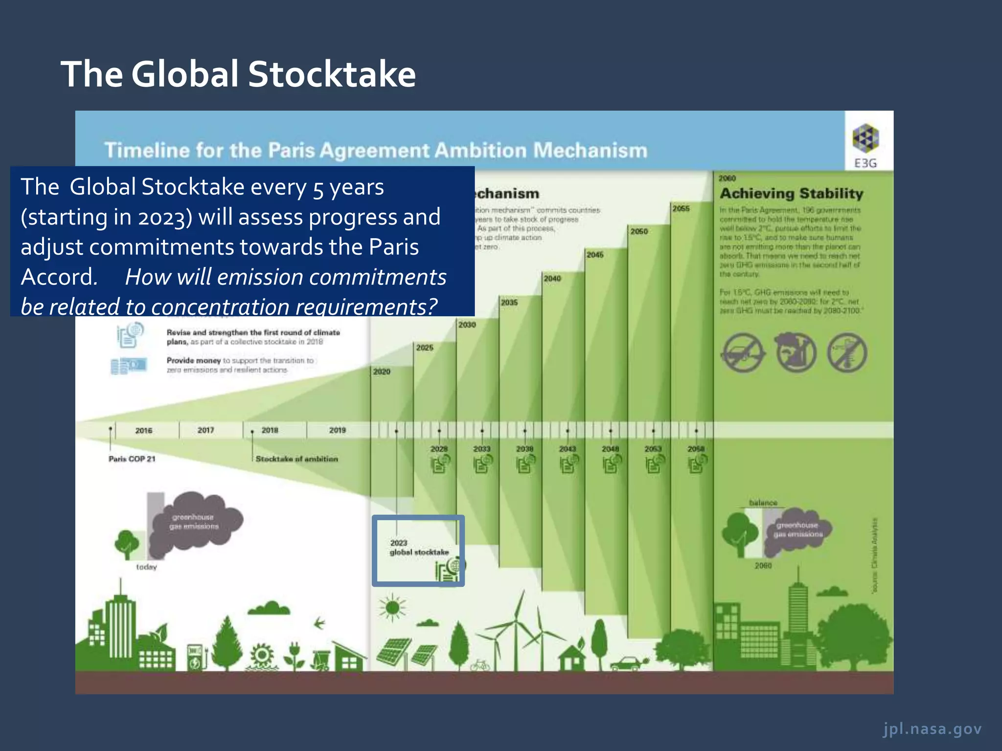
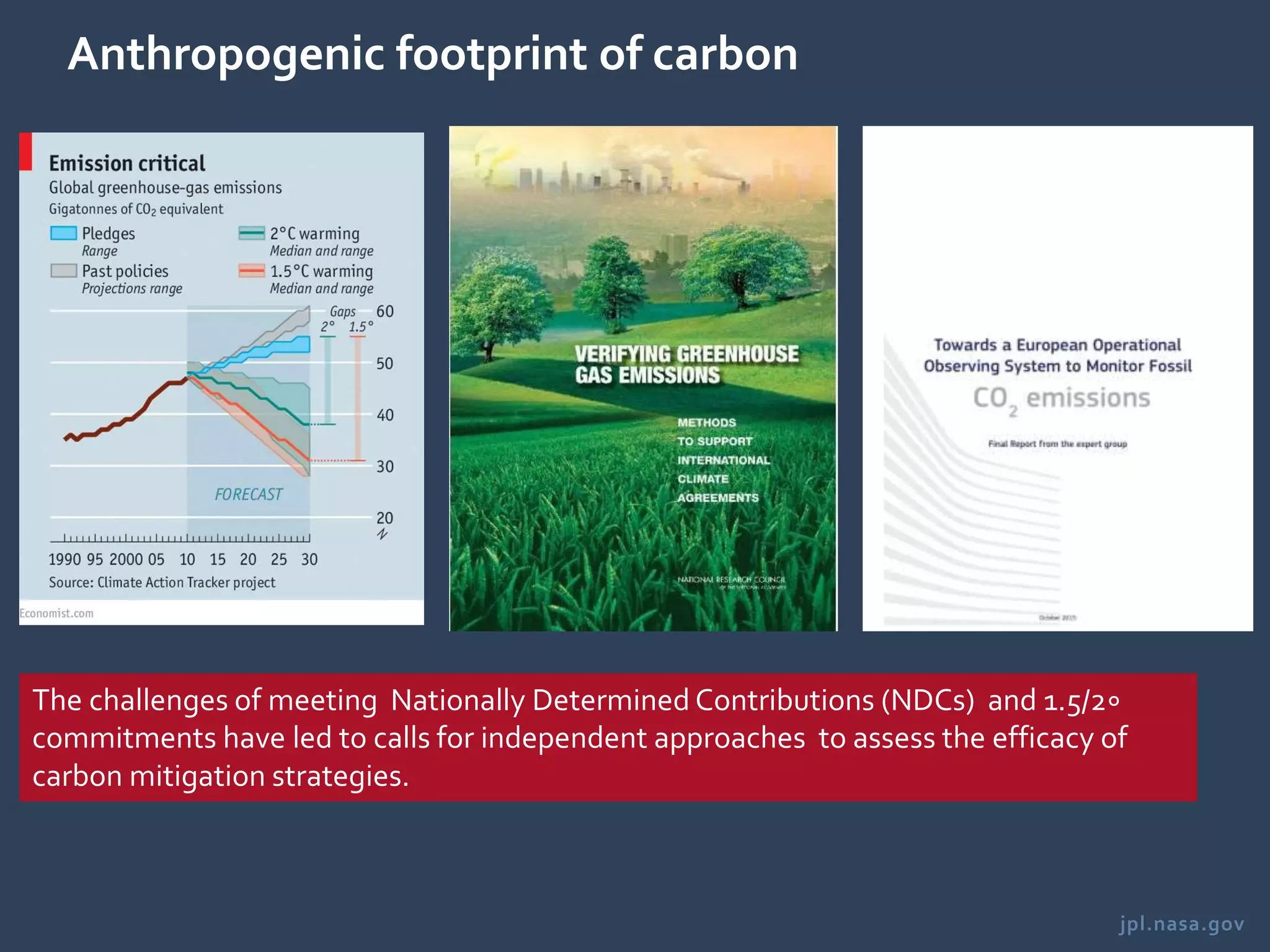
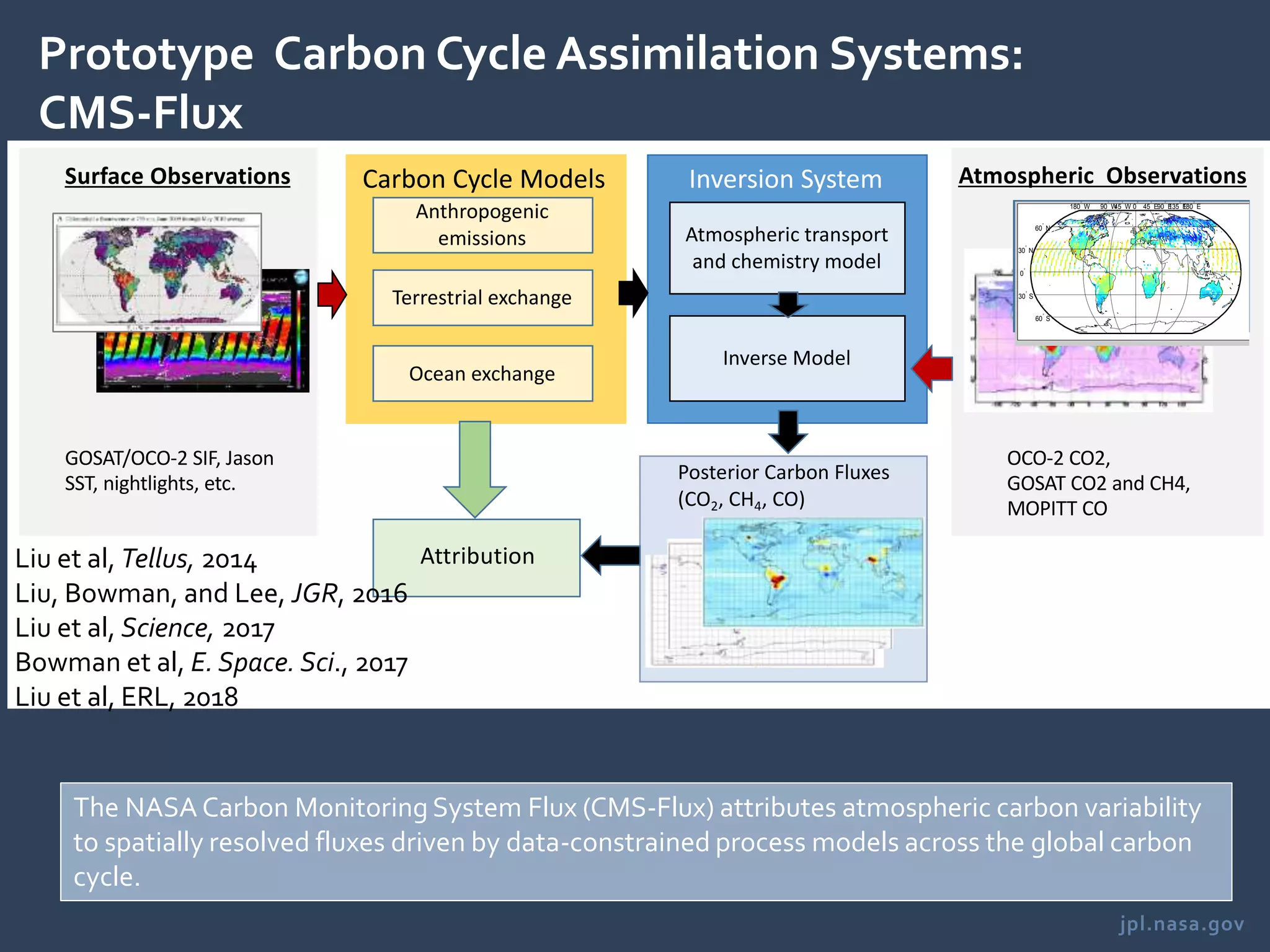
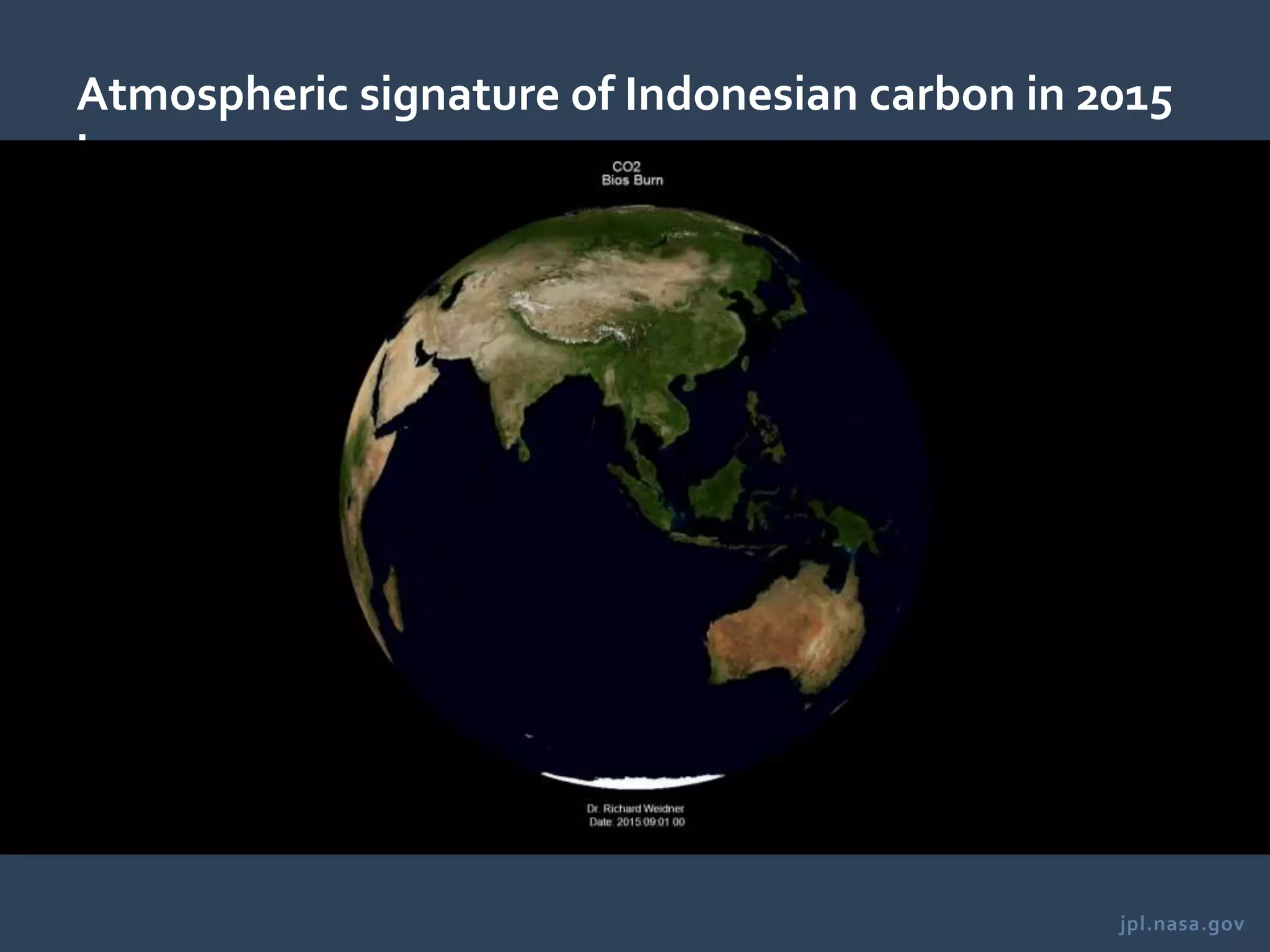
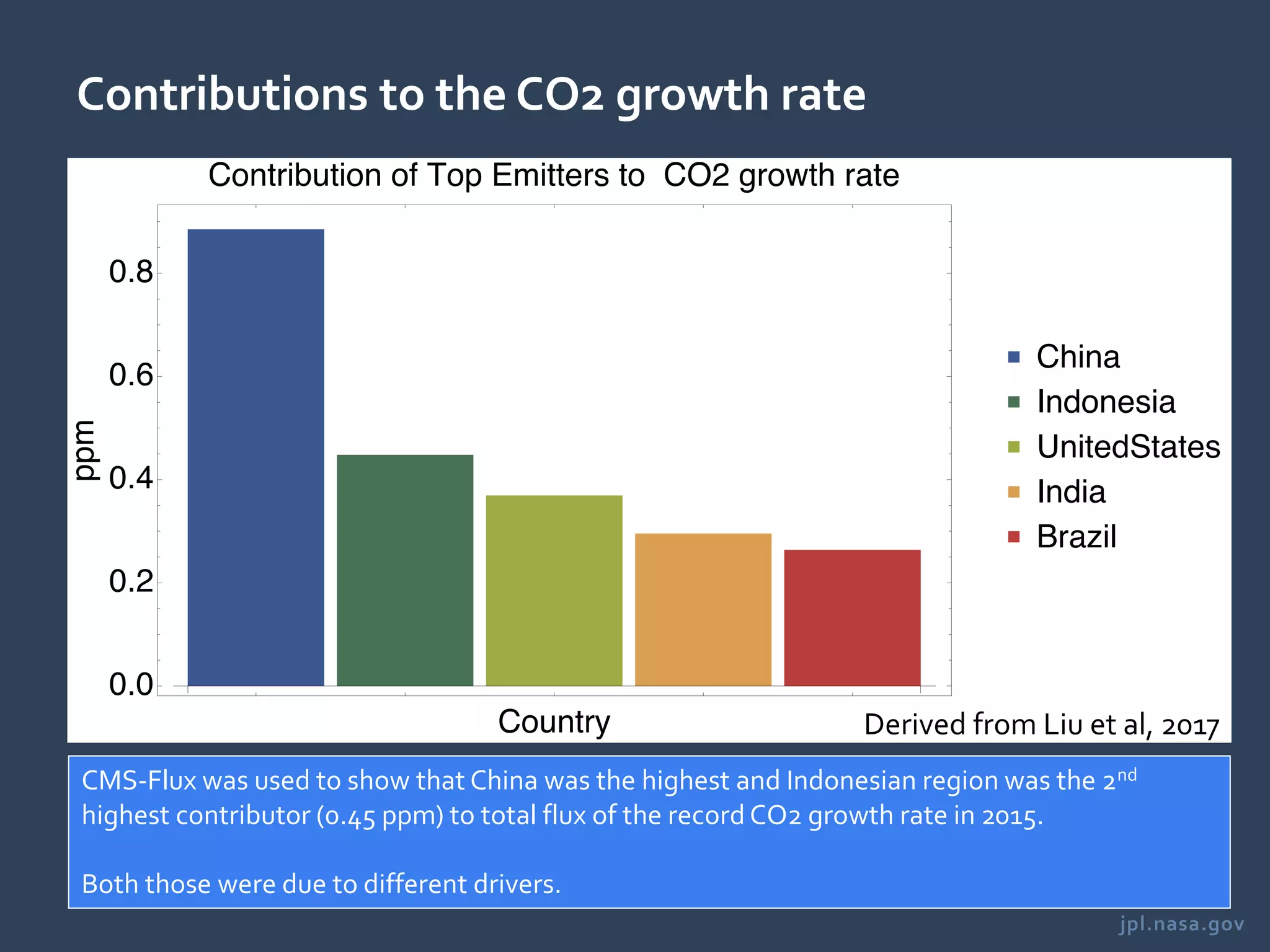
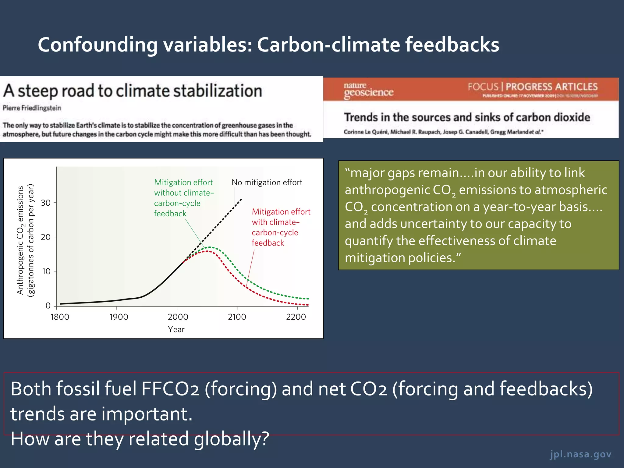
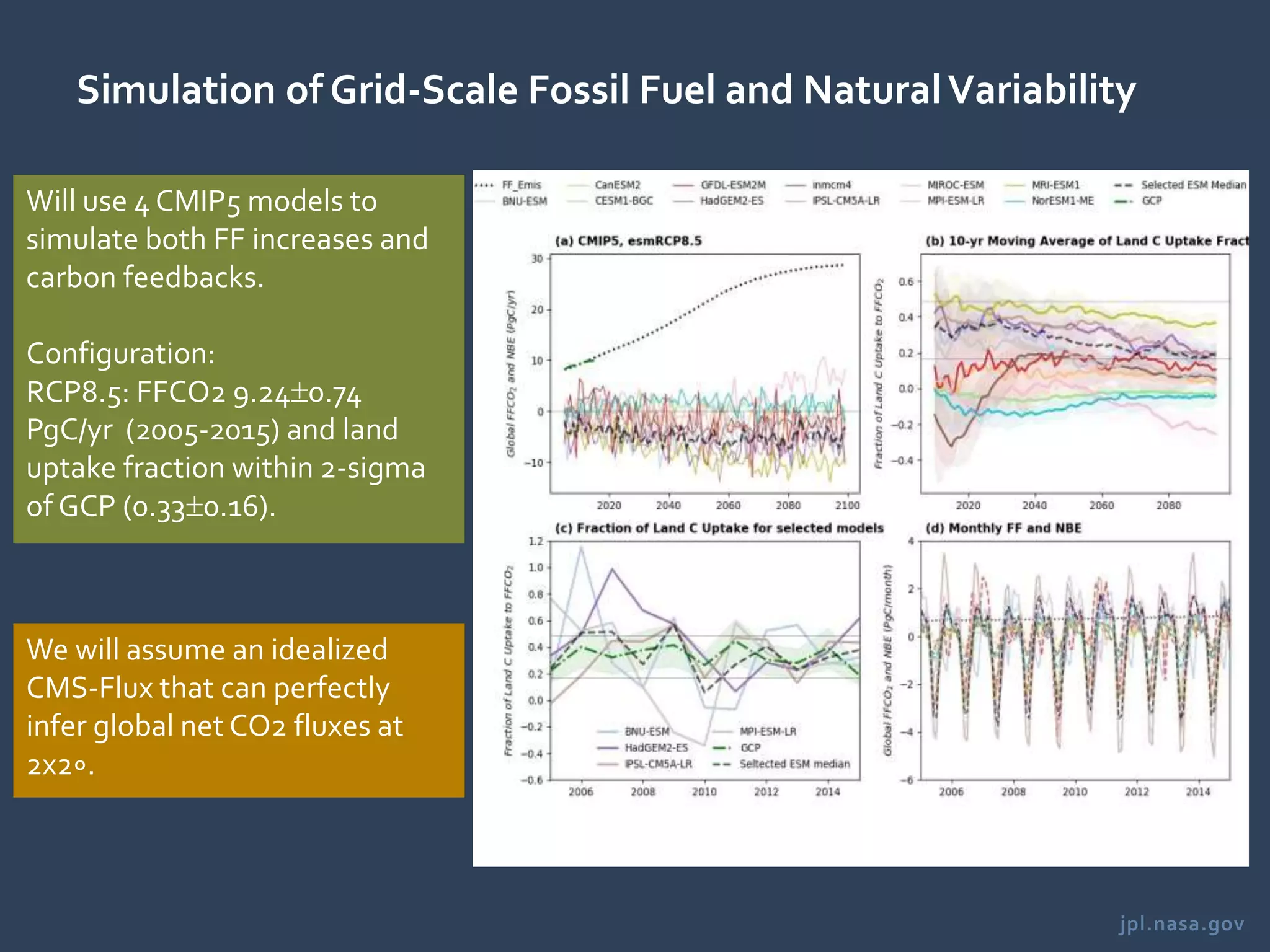
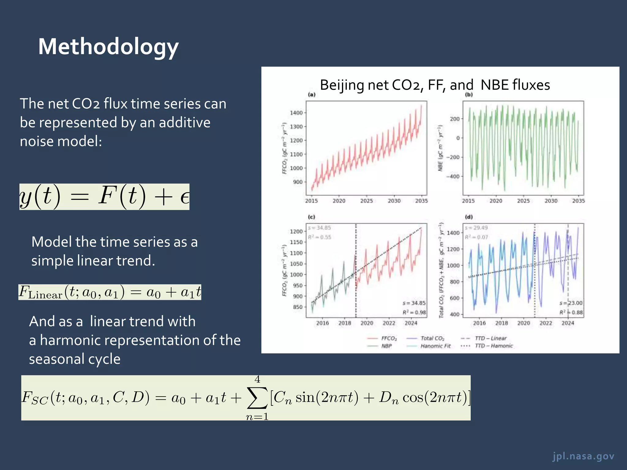
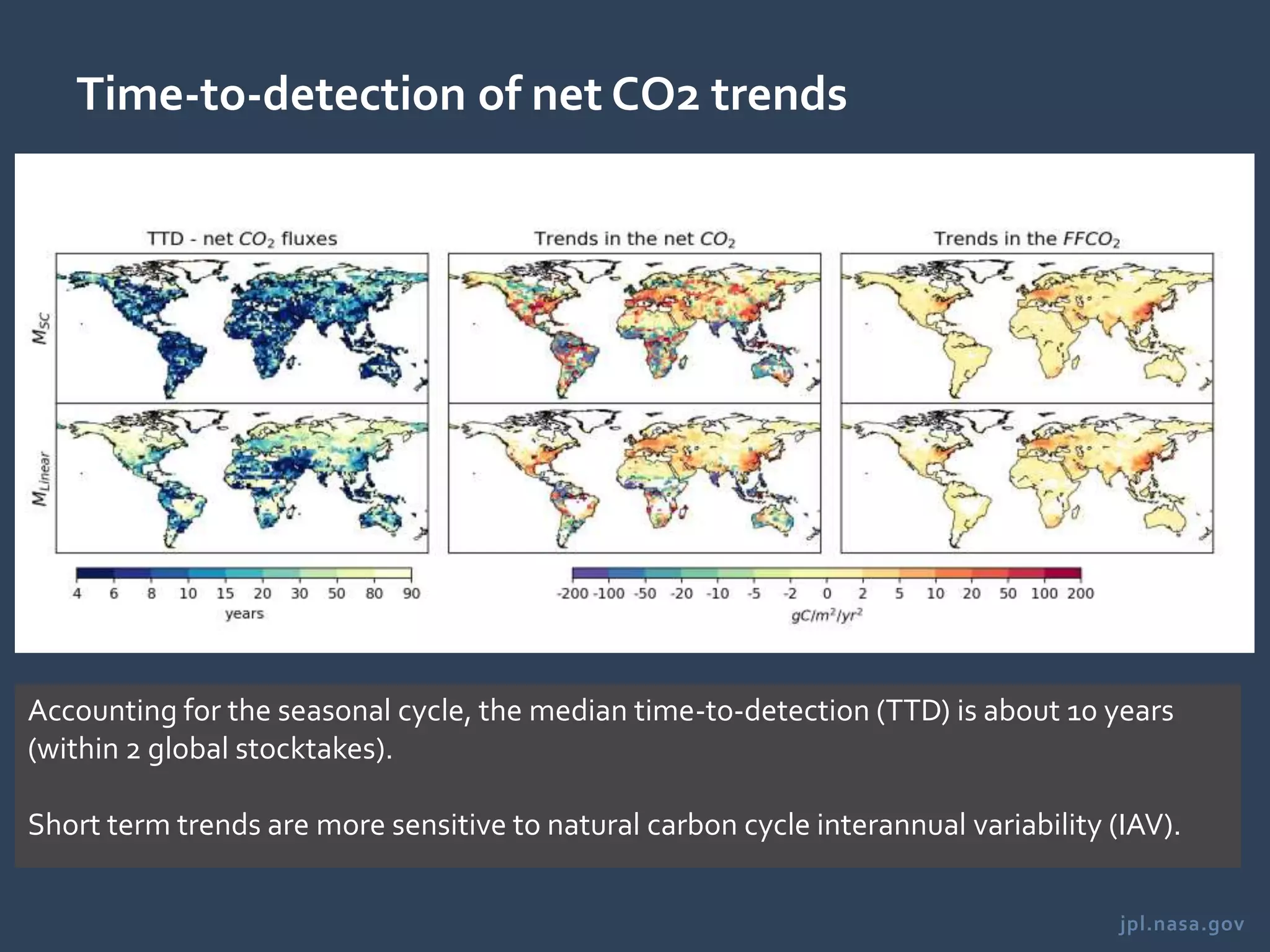
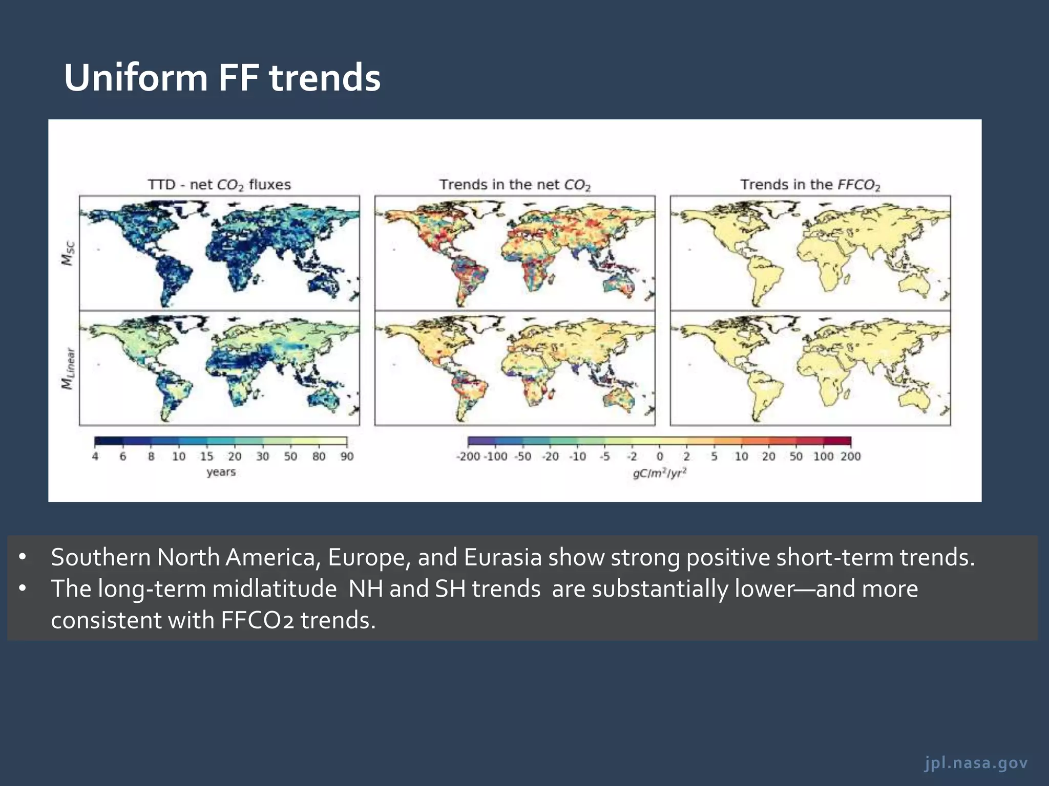
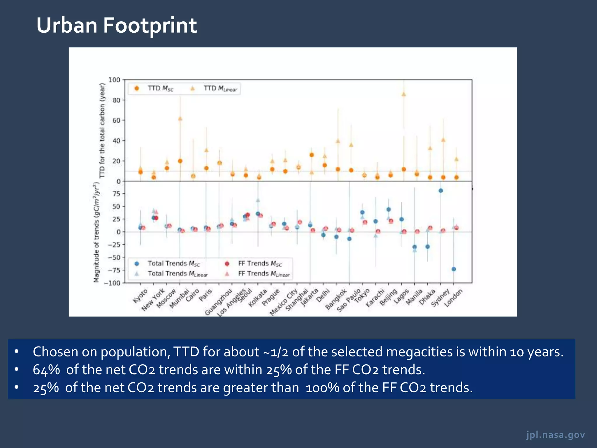
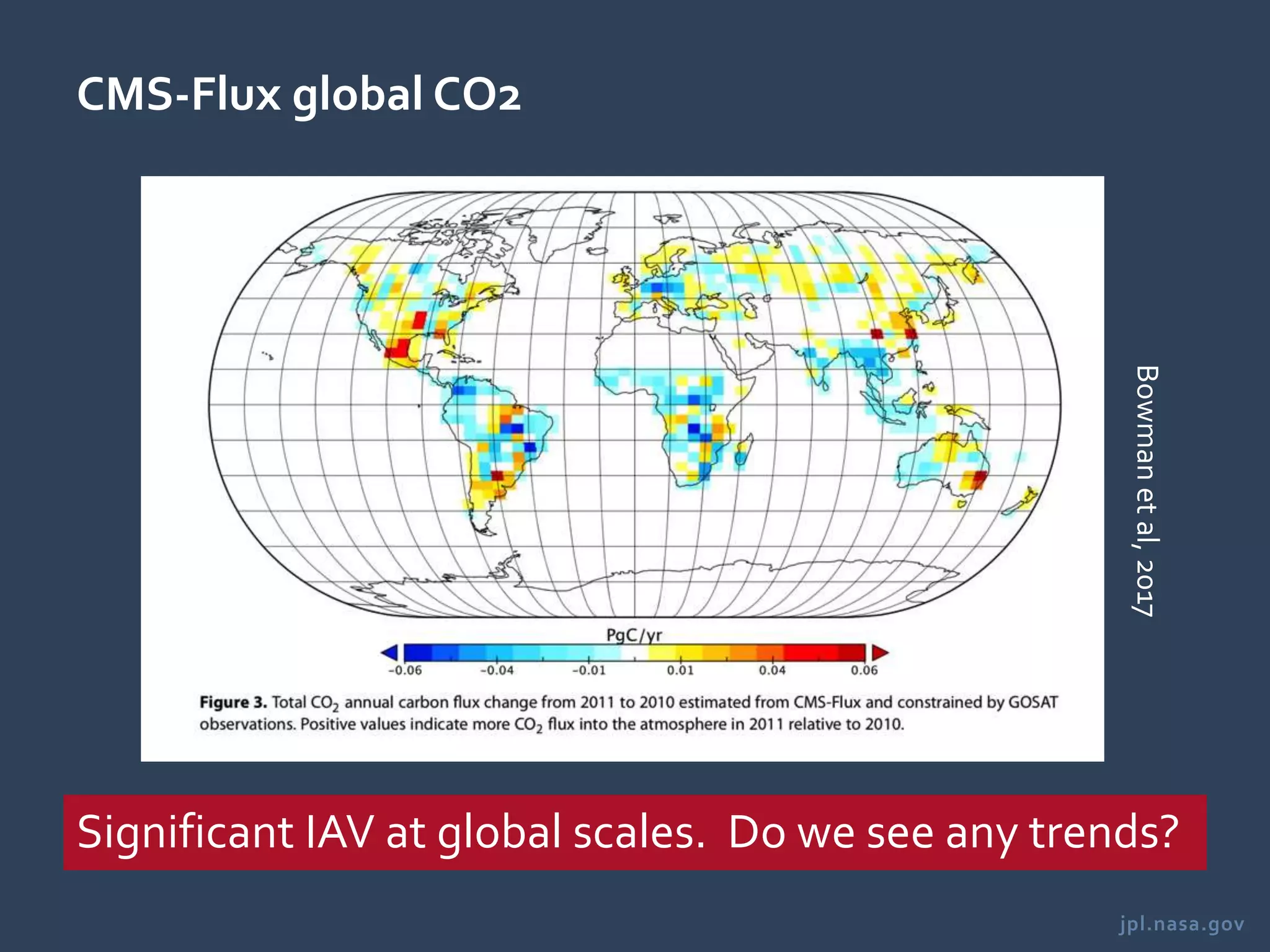
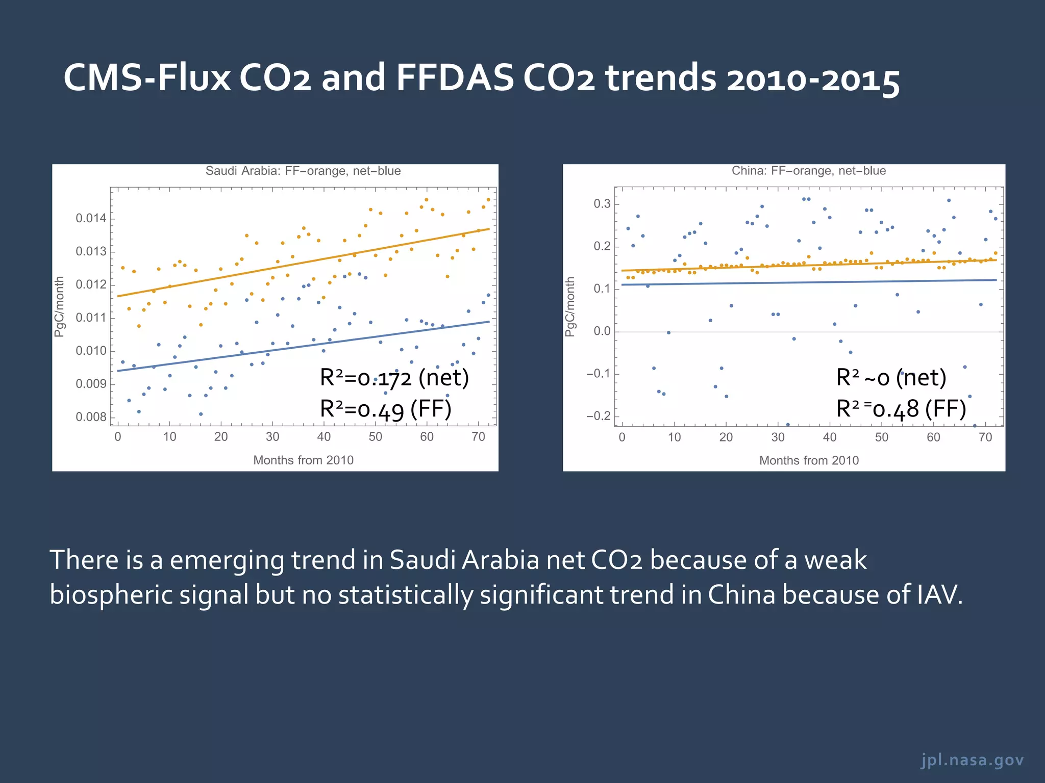
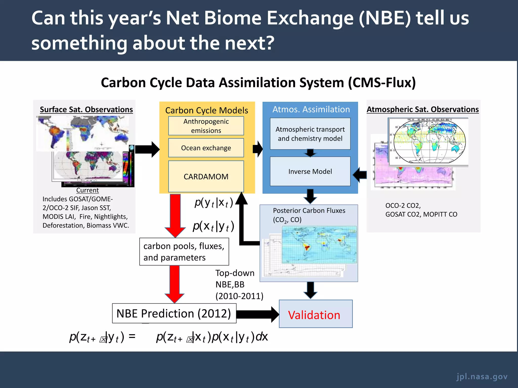
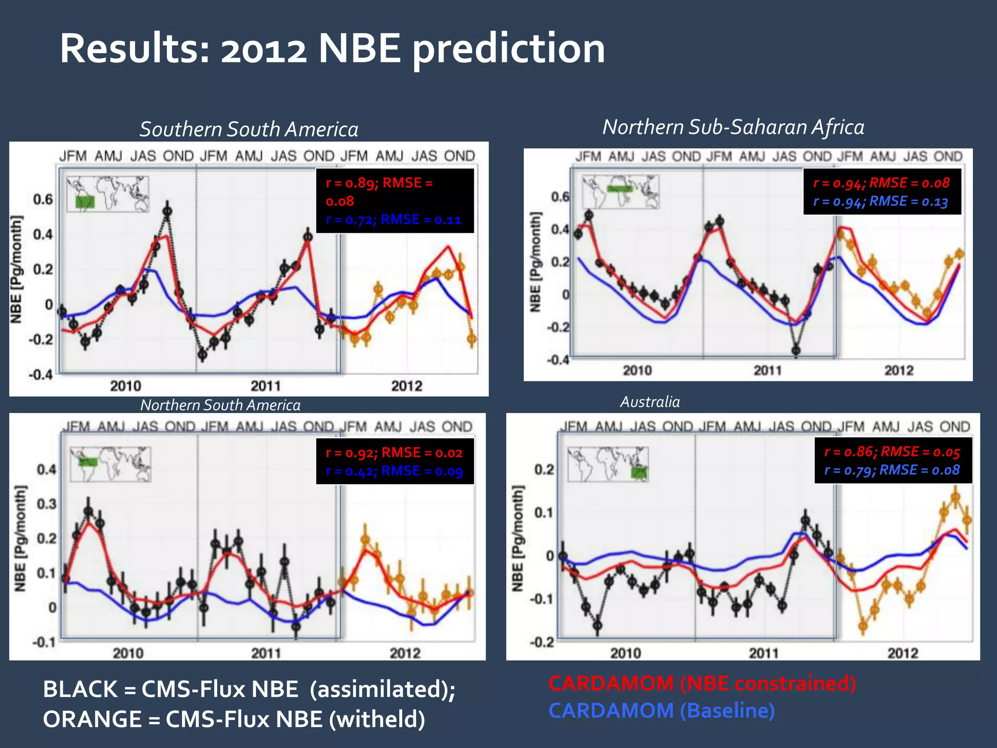
1. Detection of fossil fuel emission trends across
the globe: Challenge of natural variability
KevinW. Bowman1,2,YiYin1,3, Anthony Bloom1,Junjie Liu1, John
Worden1
1Jet Propulsion Laboratory, California Institute ofTechnology, Pasadena, CA, USA
2Joint Institute for Regional Earth System Science and Engineering, University of
California, Los Angeles, CA
3Department of Environmental Science and Engineering, California Institute of
Technology, Pasadena, CA, USA

2. jpl.nasa.gov
Climate Euphoria

3. jpl.nasa.gov
The Global Stocktake
The Global Stocktake every 5 years
(starting in 2023) will assess progress and
adjust commitments towards the Paris
Accord. How will emission commitments
be related to concentration requirements?

4. jpl.nasa.gov
Anthropogenic footprint of carbon
The challenges of meeting Nationally Determined Contributions (NDCs) and 1.5/2∘
commitments have led to calls for independent approaches to assess the efficacy of
carbon mitigation strategies.

5. jpl.nasa.gov
Surface Observations Atmospheric Observations
CMS-Flux Framework
Posterior Carbon Fluxes
(CO2, CH4, CO)
GOSAT/OCO-2 SIF, Jason
SST, nightlights, etc.
OCO-2 CO2,
GOSAT CO2 and CH4,
MOPITT CO
Carbon Cycle Models
Atmospheric transport
and chemistry model
Inverse Model
Inversion System
Attribution
180
°
W 90
°
W45
°
W 0
°
45
°
E90
°
E135
°
E180
°
E
60°
S
30
°
S
0
°
30
°
N
60
°
N
Anthropogenic
emissions
Terrestrial exchange
Ocean exchange
Prototype Carbon Cycle Assimilation Systems:
CMS-Flux
The NASA Carbon Monitoring System Flux (CMS-Flux) attributes atmospheric carbon variability
to spatially resolved fluxes driven by data-constrained process models across the global carbon
cycle.
Liu et al, Tellus, 2014
Liu, Bowman, and Lee, JGR, 2016
Liu et al, Science, 2017
Bowman et al, E. Space. Sci., 2017
Liu et al, ERL, 2018

6. jpl.nasa.gov
Atmospheric signature of Indonesian carbon in 2015
in 2

7. jpl.nasa.gov
Contributions to the CO2 growth rate
CMS-Flux was used to show that China was the highest and Indonesian region was the 2nd
highest contributor (0.45 ppm) to total flux of the record CO2 growth rate in 2015.
Both those were due to different drivers.
Derived from Liu et al, 2017

8. jpl.nasa.gov
Confounding variables: Carbon-climate feedbacks
“major gaps remain….in our ability to link
anthropogenicCO2 emissions to atmospheric
CO2 concentration on a year-to-year basis….
and adds uncertainty to our capacity to
quantify the effectiveness of climate
mitigation policies.”
Both fossil fuel FFCO2 (forcing) and net CO2 (forcing and feedbacks)
trends are important.
How are they related globally?

9. jpl.nasa.gov
Simulation of Grid-Scale Fossil Fuel and NaturalVariability
Will use 4 CMIP5 models to
simulate both FF increases and
carbon feedbacks.
Configuration:
RCP8.5: FFCO2 9.240.74
PgC/yr (2005-2015) and land
uptake fraction within 2-sigma
of GCP (0.330.16).
We will assume an idealized
CMS-Flux that can perfectly
infer global net CO2 fluxes at
2x2∘.

10. jpl.nasa.gov
Methodology
The net CO2 flux time series can
be represented by an additive
noise model:
Beijing net CO2, FF, and NBE fluxes
Model the time series as a
simple linear trend.
And as a linear trend with
a harmonic representation of the
seasonal cycle

11. jpl.nasa.gov
Time-to-detection of net CO2 trends
Accounting for the seasonal cycle, the median time-to-detection (TTD) is about 10 years
(within 2 global stocktakes).
Short term trends are more sensitive to natural carbon cycle interannual variability (IAV).

12. jpl.nasa.gov
Uniform FF trends
• Southern North America, Europe, and Eurasia show strong positive short-term trends.
• The long-term midlatitude NH and SH trends are substantially lower—and more
consistent with FFCO2 trends.

13. jpl.nasa.gov
Regional variations in trends
For, FFCO2 trends greater than 5
gC/m2/yr2 , ~1/3 corresponding
net CO2 trends agree to within
25%.
Similarly in China, ~20% of the
net CO2 trends agree to within
25%.
In the Middle East, over 70% of
net CO2 trends is within 25%
There is a wide intra-regional
range of TTD with the Middle East
having the lowest range 5 years(5-
10 1st and 3rd quartile), though
Europe and ChinaTTD 3rd quartile
is within 20 years.

14. jpl.nasa.gov
Urban Footprint
• Chosen on population,TTD for about ~1/2 of the selected megacities is within 10 years.
• 64% of the net CO2 trends are within 25% of the FF CO2 trends.
• 25% of the net CO2 trends are greater than 100% of the FF CO2 trends.

15. jpl.nasa.gov
What about now?

16. jpl.nasa.gov
CMS-Flux global CO2
Bowmanetal,2017
Significant IAV at global scales. Do we see any trends?

17. jpl.nasa.gov
CMS-Flux CO2 and FFDAS CO2 trends 2010-2015
R2=0.172 (net)
R2=0.49 (FF)
R2 ~0 (net)
R2 =0.48 (FF)
There is a emerging trend in Saudi Arabia net CO2 because of a weak
biospheric signal but no statistically significant trend in China because of IAV.

18. jpl.nasa.gov
Conclusions/Future Directions
• The bidecadal stocktake will require a link between
• net CO2 flux   Concentrations (what the climate sees)
• FFCO2   Emissions (what carbon mitigation sees)
• Systems like CMS-Flux, ECMWF, etc. could potentially attribute
CO2 growth rate trends to regionally net CO2 flux trends within
two stocktakes.
• Critically dependent on increasing observational density and reducing
systematic error.
• Could also contribute to FFCO2 for large temporal gradients, esp. in
arid regions
• Improved prediction of IAV—harnessing solar induced fluorescence
(SIF), biomass, etc.--will be critical for wider application. (Progress in
CMS-Flux)
• Preliminary analysis suggests a net CO2 trend in Saudi Arabia.
• Utilization of ancillary measurements, e.g., NO2 and CO, will be
necessary

19. jpl.nasa.gov

20. jpl.nasa.gov
Can this year’s Net Biome Exchange (NBE) tell us
something about the next?
180
°
W 90
°
W45
°
W 0
°
45
°
E90
°
E135
°
E180
°
E
60°
S
30
°
S
0
°
30
°
N
60
°
N
380
385
390
395
mates improve on forest carbon stock estimates reported pre-
viously (8, 13–15, 17, 18, 25) by providing a traceable and sys-
tematic approach to geographically locate the stock estimates for
further monitoring and verification. The forest definitions chosen
here using tree cover thresholds can readily change the estimates
of total carbon and area-weighted carbon densities at national
and regional scales.
Uncertain ty Analysis. We assess the accuracy of the biomass car-
bon estimates by calculating the error as the difference between
the true mean biomass value (bootstrapped samples of ground
and Lidar-estimated AGB) and the predicted biomass value
(mapped at 1-km grid cell resolution) and propagating these
errors through the spatial modeling process (SI Materials and
Methods). Errors in the distribution of forest aboveground bio-
mass can be random or systematic in nature and can include the
following: (i) observation errors associated with the uncertainty in
estimates of Lorey’s height from GLAS Lidar, errors associated
with estimating AGB derived from GLAS Lidar height, and
errors in estimating BGB from AGB (27); (ii) sampling errors
associated with the spatial variability of AGB within a 1-km pixel
and the representativeness and size of inventory plotsand GLAS
pixels over the landscape (29); and (iii ) prediction errors associ-
ated with spatial analysis and mapping of AGB from significant
contributions from satellite imagery (Fig. S3) (14, 30). We
combined these three types of errors (SI Materials and Methods)
to quantify the uncertainty of total biomass carbon stock as the
95% bootstrapped confidence interval at the 1-km pixel level
(Fig. 3B). The overall uncertainty in mapping AGB at the pixel
scale averaged over all continental regions is estimated at ± 30%,
but it is not uniform across regions or AGB ranges (± 6% to
±53%) and depends on regional variations of forests, quality of
remote sensing imagery, and sampling size and distribution of
available ground and GLAS data. However, when averaged over
all AGB ranges, regional uncertainties were comparable: ±27%
over Latin America, ±32% over Africa, and ±33% over Asia
(Fig. S4). The uncertainty in total carbon stock at the pixel scale
averaged ±38% over all three continents after errors associated
with BGB estimation were included in the analysis.
We computed the uncertainty around carbon estimates at
national and regional scales by propagating errors associated
with observation, including the errors associated with BGB
estimates, sampling, and prediction. The uncertainty of carbon
stock estimates at the national level was calculated as the square
root of the sum of per-pixel errors for all pixels within the na-
tional boundary. This process reduced the relative errors as
sample area increased. The national estimates were found to be
constrained to within ±1% of the total carbon stock obtained
Fig. 3. Benchmar k map of carbon stock and uncertainty. (A) Forest carbon stock defined as 50% of AGB + BGB is mapped at 1-km pixel resolution and
colored on the basisof a 12–25 Mg Cha−1
range to show the spatial patterns. (B) The uncertainty of the benchmark map isestimated using error propagation
through a spatial modeling approach. The uncertainty is given in terms of plus or minus percent and it includes all errors associated with prediction from
spatial modeling, estimation of Lorey’s height from GLAS, estimation of AGB from Lorey’sheight, errors from pixel level variati ons, and errors associated with
BGB estimation (SI Materials and Methods).
4 of 6 | www.pnas.org/cgi/doi /10.1073/pnas.101957610 8 Saatchi et al.
p(zt + ⌧|yt ) =
Z
p(zt + ⌧|xt )p(xt |yt )dx
p(yt |xt )
p(xt |yt )

21. Results: 2012 NBE prediction
BLACK = CMS-Flux NBE (assimilated);
ORANGE = CMS-Flux NBE (witheld)
CARDAMOM (NBE constrained)
CARDAMOM (Baseline)
r = 0.86; RMSE = 0.05
r = 0.79; RMSE = 0.08
r = 0.94; RMSE = 0.08
r = 0.94; RMSE = 0.13
r = 0.92; RMSE = 0.02
r = 0.42; RMSE = 0.09
r = 0.89; RMSE =
0.08
r = 0.72; RMSE = 0.11
Southern South America
Northern South America Australia
Northern Sub-Saharan Africa

22. jpl.nasa.gov
Toward an Air Quality-Carbon-Climate
Constellation
• LEO:
• IASI+GOME-2, AIRS+OMI, CrIS+OMPS could provide UV+IR ozone products for more than a decade.
• Combined UV+IR ozone products fromGEO-UVN and GEO-TIR aboard Sentinel 4 (Ingmann et al, 2012 Atm. Env.)
• Sentinel 5p (TROPOMI) will provide column CO and CH4.
• OCO-2+AIRS, GOSAT II (IR+NIR) could provide vertical discrimination.
• GEO
• TEMPO, Sentinel-4, and GEMS, would provide high spatio-temporal air quality information.
• GeoCarb and G3E could provide geo-carbon information.
Bowmanetal,Atm.Env.2013
OCO-2, OCO-3, GOSAT II/III, MERLIN
Sentinel 7,TANSAT,…
GeoCarb G3E?
???
Biomass?
Water?

23. jpl.nasa.gov
Climate-Climate Framework
GHG inventories &
reporting
Project-level
forest carbon
data
Measurement, Reporting &Verification
(MRV) frameworks
2015 202X?
Total
Carbon
Climate
Variability
Climate
Feedback
Carbon Cycle Framework
Anthropogenic
and natural
terrestrial
GEOS-5