Ch.10

10-1

Chapter 10
VAPOR AND COMBINED POWER CYCLES

Carnot Vapor Cycle

10-1C Because excessive moisture in steam causes erosion on the turbine blades. The highest moisture
content allowed is about 10%.

10-2C The Carnot cycle is not a realistic model for steam power plants because (1) limiting the heat
transfer processes to two-phase systems to maintain isothermal conditions severely limits the maximum
temperature that can be used in the cycle, (2) the turbine will have to handle steam with a high moisture
content which causes erosion, and (3) it is not practical to design a compressor that will handle two phases.

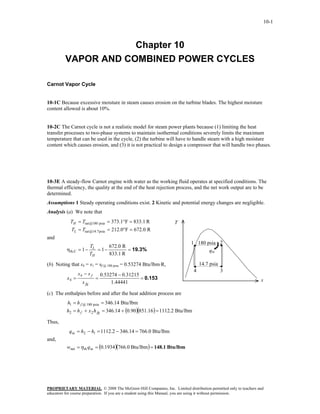
10-3E A steady-flow Carnot engine with water as the working fluid operates at specified conditions. The
thermal efficiency, the quality at the end of the heat rejection process, and the net work output are to be
determined.
Assumptions 1 Steady operating conditions exist. 2 Kinetic and potential energy changes are negligible.
Analysis (a) We note that
TH = Tsat @180 psia = 373.1°F = 833.1 R T
TL = Tsat @14.7 psia = 212.0°F = 672.0 R
and
1 180 psia 2
T 672.0 R
ηth,C = 1− L = 1− = 19.3% qin
TH 833.1 R

(b) Noting that s4 = s1 = sf @ 180 psia = 0.53274 Btu/lbm·R, 14.7 psia
4 3
s4 − s f 0.53274 − 0.31215
x4 = = = 0.153 s
s fg 1.44441

(c) The enthalpies before and after the heat addition process are
h1 = h f @ 180 psia = 346.14 Btu/lbm
h2 = h f + x 2 h fg = 346.14 + (0.90)(851.16) = 1112.2 Btu/lbm

Thus,
q in = h2 − h1 = 1112.2 − 346.14 = 766.0 Btu/lbm
and,
wnet = η th q in = (0.1934)(766.0 Btu/lbm) = 148.1 Btu/lbm

PROPRIETARY MATERIAL. © 2008 The McGraw-Hill Companies, Inc. Limited distribution permitted only to teachers and
educators for course preparation. If you are a student using this Manual, you are using it without permission.

10-2

10-4 A steady-flow Carnot engine with water as the working fluid operates at specified conditions. The
thermal efficiency, the amount of heat rejected, and the net work output are to be determined.
Analysis (a) Noting that TH = 250°C = 523 K and TL = Tsat @ 20 kPa = 60.06°C = 333.1 K, the thermal
efficiency becomes
TL 333.1 K
η th,C = 1 − = 1− = 0.3632 = 36.3% T
TH 523 K

(b) The heat supplied during this cycle is simply the
enthalpy of vaporization, 2
1
250°C
q in = h fg @ 250oC = 1715.3 kJ/kg qin
Thus,
⎛ 333.1 K ⎞ 20 kPa
⎜ 523 K ⎟(1715.3 kJ/kg ) = 1092.3 kJ/kg
TL
q out = q L = q in = ⎜ ⎟ 4 3
TH ⎝ ⎠ qout
s
(c) The net work output of this cycle is
wnet = η th q in = (0.3632 )(1715.3 kJ/kg ) = 623.0 kJ/kg

thermal efficiency, the amount of heat rejected, and the net work output are to be determined.
Analysis (a) Noting that TH = 250°C = 523 K and TL = Tsat @ 10 kPa = 45.81°C = 318.8 K, the thermal
efficiency becomes
TL 318.8 K
η th, C = 1 − =1− = 39.04% T
TH 523 K

(b) The heat supplied during this cycle is simply the
enthalpy of vaporization, 1 2
250°C
q in = h fg @ 250°C = 1715.3 kJ/kg qin
Thus,
⎛ 318.8 K ⎞ 10 kPa
⎜ 523 K ⎟(1715.3 kJ/kg ) = 1045.6 kJ/kg
TL
q out = q L = q in = ⎜ ⎟ 4 3
TH ⎝ ⎠ qout
s
(c) The net work output of this cycle is
wnet = η th q in = (0.3904)(1715.3 kJ/kg ) = 669.7 kJ/kg


10-3

thermal efficiency, the pressure at the turbine inlet, and the net work output are to be determined.
Analysis (a) The thermal efficiency is determined from
TL 60 + 273 K T
η th, C = 1 − = 1− = 46.5%
TH 350 + 273 K

(b) Note that 1 2
s2 = s3 = sf + x3sfg 350°C

= 0.8313 + 0.891 × 7.0769 = 7.1368 kJ/kg·K
Thus,
60°C
4 3
T2 = 350°C ⎫ s
⎬ P2 ≅ 1.40 MPa (Table A-6)
s 2 = 7.1368 kJ/kg ⋅ K ⎭

(c) The net work can be determined by calculating the enclosed area on the T-s diagram,
s 4 = s f + x 4 s fg = 0.8313 + (0.1)(7.0769) = 1.5390 kJ/kg ⋅ K
Thus,
wnet = Area = (TH − TL )(s 3 − s 4 ) = (350 − 60)(7.1368 − 1.5390) = 1623 kJ/kg


10-4

The Simple Rankine Cycle

10-7C The four processes that make up the simple ideal cycle are (1) Isentropic compression in a pump,
(2) P = constant heat addition in a boiler, (3) Isentropic expansion in a turbine, and (4) P = constant heat
rejection in a condenser.

10-8C Heat rejected decreases; everything else increases.

10-9C Heat rejected decreases; everything else increases.

10-10C The pump work remains the same, the moisture content decreases, everything else increases.

10-11C The actual vapor power cycles differ from the idealized ones in that the actual cycles involve
friction and pressure drops in various components and the piping, and heat loss to the surrounding medium
from these components and piping.

10-12C The boiler exit pressure will be (a) lower than the boiler inlet pressure in actual cycles, and (b) the
same as the boiler inlet pressure in ideal cycles.

10-13C We would reject this proposal because wturb = h1 - h2 - qout, and any heat loss from the steam will
adversely affect the turbine work output.

10-14C Yes, because the saturation temperature of steam at 10 kPa is 45.81°C, which is much higher than
the temperature of the cooling water.


10-5

10-15E A simple ideal Rankine cycle with water as the working fluid operates between the specified
pressure limits. The rates of heat addition and rejection, and the thermal efficiency of the cycle are to be
determined.
Analysis From the steam tables (Tables A-4E, A-5E, and A-6E),
h1 = h f @ 6 psia = 138.02 Btu/lbm
v 1 = v f @ 6 psia = 0.01645 ft 3 /lbm T

wp,in = v 1 ( P2 − P1 ) 3
⎛ ⎞ 500 psia
1 Btu
= (0.01645 ft 3 /lbm)(500 − 6)psia ⎜ ⎟
⎜ 5.404 psia ⋅ ft 3 ⎟
= 1.50 Btu/lbm ⎝ ⎠ 2 qin
h2 = h1 + wp,in = 138.02 + 1.50 = 139.52 Btu/lbm 6 psia
1 4
P3 = 500 psia ⎫ h3 = 1630.0 Btu/lbm qout
⎬
T3 = 1200°F ⎭ s 3 = 1.8075 Btu/lbm ⋅ R
s
s 4 − s f 1.8075 − 0.24739
P4 = 6 psia ⎫ x 4 = = = 0.9864
⎬ s fg 1.58155
s 4 = s3 ⎭ h = h + x h = 138.02 + (0.9864)(995.88) = 1120.4 Btu/lbm
4 f 4 fg

Knowing the power output from the turbine the mass flow rate of steam in the cycle is determined from
&
&
WT,out 500 kJ/s ⎛ 0.94782 Btu ⎞
WT,out = m(h3 − h4 ) ⎯
& ⎯→ m =
& = ⎜ ⎟ = 0.9300 lbm/s
h3 − h4 (1630.0 − 1120.4)Btu/lbm ⎝ 1 kJ ⎠
The rates of heat addition and rejection are
&
Qin = m(h3 − h2 ) = (0.9300 lbm/s)(1630.0 − 139.52)Btu/lbm = 1386 Btu/s
&
& = m(h − h ) = (0.9300 lbm/s)(1120.4 − 138.02)Btu/lbm = 913.6 Btu/s
Qout & 4 1
and the thermal efficiency of the cycle is
&
Qout 913.6
η th = 1 − = 1− = 0.341
Q& 1386
in


10-6

10-16 A simple ideal Rankine cycle with water as the working fluid operates between the specified pressure
limits. The maximum thermal efficiency of the cycle for a given quality at the turbine exit is to be
determined.
Analysis For maximum thermal efficiency, the quality at state 4 would be at its minimum of 85% (most
closely approaches the Carnot cycle), and the properties at state 4 would be (Table A-5)
P4 = 30 kPa ⎫ h4 = h f + x 4 h fg = 289.27 + (0.85)(2335.3) = 2274.3 kJ/kg
⎬
x 4 = 0.85 ⎭ s 4 = s f + x 4 s fg = 0.9441 + (0.85)(6.8234) = 6.7440 kJ/kg ⋅ K

Since the expansion in the turbine is isentropic,
P3 = 3000 kPa ⎫
⎬ h3 = 3115.5 kJ/kg T
s 3 = s 4 = 6.7440 kJ/kg ⋅ K ⎭

Other properties are obtained as follows (Tables A-4, A-5, and A-6), 3
3 MPa
h1 = h f @ 30 kPa = 289.27 kJ/kg
2 qin
v 1 = v f @ 30 kPa = 0.001022 m 3 /kg
30 kPa
wp,in = v 1 ( P2 − P1 ) 1 4
⎛ 1 kJ ⎞ qout
= (0.001022 m 3 /kg )(3000 − 30)kPa ⎜ ⎟
= 3.04 kJ/kg ⎝ 1 kPa ⋅ m 3 ⎠
s
h2 = h1 + wp,in = 289.27 + 3.04 = 292.31 kJ/kg

Thus,
q in = h3 − h2 = 3115.5 − 292.31 = 2823.2 kJ/kg
q out = h4 − h1 = 2274.3 − 289.27 = 1985.0 kJ/kg

q out 1985.0
η th = 1 − = 1− = 0.297
q in 2823.2


10-7

limits. The power produced by the turbine and consumed by the pump are to be determined.
Analysis From the steam tables (Tables A-4, A-5, and A-6),
h1 = h f @ 20 kPa = 251.42 kJ/kg
v 1 = v f @ 20 kPa = 0.001017 m 3 /kg T

3
wp,in = v 1 ( P2 − P1 ) 4 MPa
⎛ 1 kJ ⎞
= (0.001017 m 3 /kg)(4000 − 20)kPa ⎜ ⎟
= 4.05 kJ/kg ⎝ 1 kPa ⋅ m 3 ⎠ 2 qin

h2 = h1 + wp,in = 251.42 + 4.05 = 255.47 kJ/kg 20 kPa
1 qout 4
P3 = 4000 kPa ⎫ h3 = 3906.3 kJ/kg
⎬
T3 = 700°C ⎭ s 3 = 7.6214 kJ/kg ⋅ K s
s4 − s f
7.6214 − 0.8320
P4 = 20 kPa ⎫ x 4 = = = 0.9596
⎬ s fg 7.0752
s 4 = s3 ⎭ h = h + x h = 251.42 + (0.9596)(2357.5) = 2513.7 kJ/kg
4 f 4 fg

The power produced by the turbine and consumed by the pump are
&
WT,out = m(h3 − h4 ) = (50 kg/s)(3906.3 − 2513.7)kJ/kg = 69,630 kW
&
&
W P,in = mwP,in = (50 kg/s)(4.05 kJ/kg) = 203 kW
&


10-8

10-18E A simple ideal Rankine cycle with water as the working fluid operates between the specified
pressure limits. The turbine inlet temperature and the thermal efficiency of the cycle are to be determined.
Assumptions 1 Steady operating conditions exist. 2
Kinetic and potential energy changes are negligible.
T
Analysis From the steam tables (Tables A-4E, A-5E,
and A-6E), 3
2500 psia
h1 = h f @ 5 psia = 130.18 Btu/lbm
v 1 = v f @ 5 psia = 0.01641 ft 3 /lbm 2 qin

wp,in = v 1 ( P2 − P1 ) 5 psia
⎛ 1 Btu ⎞
= (0.01641 ft /lbm)(2500 − 5)psia ⎜
3 ⎟ 1 qout 4
⎜ 5.404 psia ⋅ ft 3 ⎟
= 7.58 Btu/lbm ⎝ ⎠
h2 = h1 + wp,in = 130.18 + 7.58 = 137.76 Btu/lbm s

P4 = 5 psia ⎫ h4 = h f + x 4 h fg = 130.18 + (0.80)(1000.5) = 930.58 Btu/lbm
⎬
x 4 = 0.80 ⎭ s 4 = s f + x 4 s fg = 0.23488 + (0.80)(1.60894) = 1.52203 Btu/lbm ⋅ R

P3 = 2500 psia ⎫ h3 = 1450.8 Btu/lbm
⎬
s 3 = s 4 = 1.52203 Btu/lbm ⋅ R ⎭ T3 = 989.2 °F

Thus,
q in = h3 − h2 = 1450.8 − 137.76 = 1313.0 Btu/lbm
q out = h4 − h1 = 930.58 − 130.18 = 800.4 Btu/lbm

The thermal efficiency of the cycle is
q out 800.4
η th = 1 − = 1− = 0.390
q in 1313.0


10-9

limits. The power produced by the turbine, the heat added in the boiler, and the thermal efficiency of the
cycle are to be determined.
h1 = h f @ 100 kPa = 417.51 kJ/kg T
v 1 = v f @ 100 kPa = 0.001043 m 3 /kg

w p,in = v 1 ( P2 − P1 ) 15 MPa
⎛ 1 kJ ⎞ 3
= (0.001043 m 3 /kg )(15,000 − 100)kPa ⎜ ⎟ 2 qin
= 15.54 kJ/kg ⎝ 1 kPa ⋅ m 3 ⎠
100 kPa
h2 = h1 + wp,in = 417.51 + 15.54 = 433.05 kJ/kg
1 qout 4
P3 = 15,000 kPa ⎫ h3 = 2610.8 kJ/kg
⎬
x3 = 1 ⎭ s 3 = 5.3108 kJ/kg ⋅ K s
s4 − s f 5.3108 − 1.3028
P4 = 100 kPa ⎫ x 4 = = = 0.6618
⎬ s fg 6.0562
s 4 = s3 ⎭ h = h + x h = 417.51 + (0.6618)(2257.5) = 1911.5 kJ/kg
4 f 4 fg

Thus,
wT,out = h3 − h4 = 2610.8 − 1911.5 = 699.3 kJ/kg
q in = h3 − h2 = 2610.8 − 433.05 = 2177.8 kJ/kg
q out = h4 − h1 = 1911.5 − 417.51 = 1494.0 kJ/kg
q out 1494.0
η th = 1 − = 1− = 0.314
q in 2177.8


10-10

10-20 A simple Rankine cycle with water as the working fluid operates between the specified pressure
limits. The isentropic efficiency of the turbine, and the thermal efficiency of the cycle are to be determined.
h1 = h f @ 100 kPa = 417.51 kJ/kg
T
v 1 = v f @ 100 kPa = 0.001043 m 3 /kg

wp,in = v 1 ( P2 − P1 ) 15 MPa
3 ⎛ 1 kJ ⎞ 3
= (0.001043 m /kg )(15,000 − 100)kPa ⎜ ⎟ 2 qin
= 15.54 kJ/kg ⎝ 1 kPa ⋅ m 3 ⎠
h2 = h1 + wp,in = 417.51 + 15.54 = 433.05 kJ/kg 100 kPa
1 qout 4s 4
P3 = 15,000 kPa ⎫ h3 = 2610.8 kJ/kg
⎬
x3 = 1 ⎭ s 3 = 5.3108 kJ/kg ⋅ K s
s4 − s f 5.3108 − 1.3028
P4 = 100 kPa ⎫ x 4 s = = = 0.6618
⎬ s fg 6.0562
s 4 = s3 ⎭ h = h + x h = 417.51 + (0.6618)(2257.5) = 1911.5 kJ/kg
4s f 4 s fg

P4 = 100 kPa ⎫
⎬ h4 = h f + x 4 h fg = 417.51 + (0.70)(2257.5) = 1997.8 kJ/kg
x 4 = 0.70 ⎭
The isentropic efficiency of the turbine is
h3 − h4 2610.8 − 1997.8
ηT = = = 0.877
h3 − h4 s 2610.8 − 1911.5

Thus,
q in = h3 − h2 = 2610.8 − 433.05 = 2177.8 kJ/kg
q out = h4 − h1 = 1997.8 − 417.51 = 1580.3 kJ/kg

q out 1580.3
η th = 1 − = 1− = 0.274
q in 2177.8


10-11

10-21E A simple steam Rankine cycle operates between the specified pressure limits. The mass flow rate,
the power produced by the turbine, the rate of heat addition, and the thermal efficiency of the cycle are to
be determined.
h1 = h f @ 1 psia = 69.72 Btu/lbm
v 1 = v f @ 6 psia = 0.01614 ft 3 /lbm T

wp,in = v 1 ( P2 − P1 ) 3
2500 psia
⎛ 1 Btu ⎞
= (0.01614 ft 3 /lbm)(2500 − 1)psia ⎜ ⎟
⎜ 5.404 psia ⋅ ft 3 ⎟
= 7.46 Btu/lbm ⎝ ⎠ 2 qin
1 4s 4
P3 = 2500 psia ⎫ h3 = 1302.0 Btu/lbm qout
⎬
T3 = 800°F ⎭ s 3 = 1.4116 Btu/lbm ⋅ R
s
s 4 − s f 1.4116 − 0.13262
P4 = 1 psia ⎫ x 4 s = = = 0.6932
⎬ s fg 1.84495
s 4 = s3 ⎭ h = h + x h = 69.72 + (0.6932)(1035.7) = 787.70 Btu/lbm
4s f 4 s fg

h3 − h4
ηT = ⎯→ h4 = h3 − η T (h3 − h4s ) = 1302.0 − (0.90)(1302.0 − 787.70) = 839.13 kJ/kg
⎯
h3 − h4 s

Thus,
q in = h3 − h2 = 1302.0 − 77.18 = 1224.8 Btu/lbm
q out = h4 − h1 = 839.13 − 69.72 = 769.41 Btu/lbm
wnet = q in − q out = 1224.8 − 769.41 = 455.39 Btu/lbm
The mass flow rate of steam in the cycle is determined from

W& 1000 kJ/s ⎛ 0.94782 Btu ⎞
& & ⎯→ m = net =
W net = mwnet ⎯ & ⎜ ⎟ = 2.081 lbm/s
wnet 455.39 Btu/lbm ⎝ 1 kJ ⎠
The power output from the turbine and the rate of heat addition are

& ⎛ 1 kJ ⎞
WT,out = m(h3 − h4 ) = (2.081 lbm/s)(1302.0 − 839.13)Btu/lbm⎜
& ⎟ = 1016 kW
⎝ 0.94782 Btu ⎠
&
Qin = mq in = (2.081 lbm/s)(1224.8 Btu/lbm) = 2549 Btu/s
&

&
W net 1000 kJ/s ⎛ 0.94782 Btu ⎞
η th = = ⎜ ⎟ = 0.3718
&
Qin 2549 Btu/s ⎝ 1 kJ ⎠


10-12

10-22E A simple steam Rankine cycle operates between the specified pressure limits. The mass flow rate,
the power produced by the turbine, the rate of heat addition, and the thermal efficiency of the cycle are to
be determined.
h1 = h f @ 1 psia = 69.72 Btu/lbm
v 1 = v f @ 6 psia = 0.01614 ft 3 /lbm T

3
wp,in = v 1 ( P2 − P1 ) 2500 psia
⎛ 1 Btu ⎞
= (0.01614 ft 3 /lbm)(2500 − 1)psia ⎜ ⎟
⎜ 5.404 psia ⋅ ft 3 ⎟ 2 qin
= 7.46 Btu/lbm ⎝ ⎠
1 qout 4s 4
P3 = 2500 psia ⎫ h3 = 1302.0 Btu/lbm
⎬
T3 = 800°F ⎭ s 3 = 1.4116 Btu/lbm ⋅ R s
s 4 − s f 1.4116 − 0.13262
P4 = 1 psia ⎫ x 4 s = = = 0.6932
⎬ s fg 1.84495
s 4 = s3 ⎭ h = h + x h = 69.72 + (0.6932)(1035.7) = 787.70 Btu/lbm
4s f 4 s fg

h3 − h4
ηT = ⎯→ h4 = h3 − η T (h3 − h4s ) = 1302.0 − (0.90)(1302.0 − 787.70) = 839.13 kJ/kg
⎯
h3 − h4 s

&
W net 1000 kJ/s ⎛ 0.94782 Btu ⎞
&
W net = m(h3 − h4 ) ⎯
& ⎯→ m =
& = ⎜ ⎟ = 2.048 lbm/s
h3 − h4 (1302.0 − 839.13) Btu/lbm ⎝ 1 kJ ⎠
The rate of heat addition is

& ⎛ 1 kJ ⎞
Qin = m(h3 − h2 ) = (2.048 lbm/s)(1302.0 − 77.18)Btu/lbm⎜
& ⎟ = 2508 Btu/s
⎝ 0.94782 Btu ⎠

&
W net 1000 kJ/s ⎛ 0.94782 Btu ⎞
η th = = ⎜ ⎟ = 0.3779
&
Qin 2508 Btu/s ⎝ 1 kJ ⎠
The thermal efficiency in the previous problem was determined to be 0.3718. The error in the thermal
efficiency caused by neglecting the pump work is then
0.3779 − 0.3718
Error = × 100 = 1.64%
0.3718


10-13

10-23 A 300-MW coal-fired steam power plant operates on a simple ideal Rankine cycle between the
specified pressure limits. The overall plant efficiency and the required rate of the coal supply are to be
determined.
Analysis (a) From the steam tables (Tables A-4, A-5, and A-6),
h1 = h f @ 25 kPa = 271.96 kJ/kg
v 1 = v f @ 25 kPa = 0.001020 m 3 /kg T

w p ,in = v 1 (P2 − P1 ) 3
( 3
)
= 0.00102 m /kg (5000 − 25 kPa )⎜
⎛ 1 kJ
⎜ 1 kPa ⋅ m 3
⎞
⎟
⎟
5 MPa
·
= 5.07 kJ/kg ⎝ ⎠ Qin
2
h2 = h1 + w p ,in = 271.96 + 5.07 = 277.03 kJ/kg
25 kPa
P3 = 5 MPa ⎫ h3 = 3317.2 kJ/kg 1 · 4
Qout
⎬
T3 = 450°C ⎭ s 3 = 6.8210 kJ/kg ⋅ K s
P4 = 25 kPa ⎫ s 4 − s f 6.8210 − 0.8932
⎬ x4 = = = 0.8545
s 4 = s3 ⎭ s fg 6.9370
h4 = h f + x 4 h fg = 271.96 + (0.8545)(2345.5) = 2276.2 kJ/kg

The thermal efficiency is determined from
qin = h3 − h2 = 3317.2 − 277.03 = 3040.2 kJ/kg
qout = h4 − h1 = 2276.2 − 271.96 = 2004.2 kJ/kg

and
q out 2004.2
η th = 1 − = 1− = 0.3407
q in 3040.2
Thus,
η overall = η th ×η comb ×η gen = (0.3407 )(0.75)(0.96 ) = 24.5%

(b) Then the required rate of coal supply becomes
&
W net 300,000 kJ/s
&
Qin = = = 1,222,992 kJ/s
η overall 0.2453
and
&
Qin 1,222,992 kJ/s ⎛ 1 ton ⎞
m coal =
& = ⎜ ⎟ = 0.04174 tons/s = 150.3 tons/h
C coal 29,300 kJ/kg ⎜ 1000 kg ⎟
⎝ ⎠


10-14

10-24 A solar-pond power plant that operates on a simple ideal Rankine cycle with refrigerant-134a as the
working fluid is considered. The thermal efficiency of the cycle and the power output of the plant are to be
determined.
Analysis (a) From the refrigerant tables (Tables A-11, A-12, and A-13),
h1 = h f @ 0.7 MPa = 88.82 kJ/kg
v 1 = v f @ 0.7 MPa = 0.0008331 m 3 /kg T
w p ,in = v 1 (P2 − P1 )

( ) ⎛ 1 kJ
= 0.0008331 m 3 /kg (1400 − 700 kPa )⎜
⎜ 1 kPa ⋅ m 3
⎞
⎟
⎟ 1.4 MPa 3
⎝ ⎠
qin
= 0.58 kJ/kg
2 R-134a
h2 = h1 + w p ,in = 88.82 + 0.58 = 89.40 kJ/kg 0.7 MPa
1 qout 4
P3 = 1.4 MPa ⎫ h3 = h g @ 1.4 MPa = 276.12 kJ/kg s
⎬
sat.vapor ⎭ s 3 = s g @ 1.4 MPa = 0.9105 kJ/kg ⋅ K
P4 = 0.7 MPa ⎫ s 4 − s f 0.9105 − 0.33230
⎬ x4 = = = 0.9839
s 4 = s3 ⎭ s fg 0.58763
h4 = h f + x 4 h fg = 88.82 + (0.9839)(176.21) = 262.20 kJ/kg

Thus ,
q in = h3 − h2 = 276.12 − 89.40 = 186.72 kJ/kg
q out = h4 − h1 = 262.20 − 88.82 = 173.38 kJ/kg
wnet = q in − q out = 186.72 − 173.38 = 13.34 kJ/kg
and
wnet 13.34 kJ/kg
η th = = = 7.1%
q in 186.72 kJ/kg

(b) Wnet = mwnet = (3 kg/s )(13.34 kJ/kg ) = 40.02 kW
& &


10-15

10-25 A steam power plant operates on a simple ideal Rankine cycle between the specified pressure limits.
The thermal efficiency of the cycle, the mass flow rate of the steam, and the temperature rise of the cooling
water are to be determined.
h1 = h f @ 10 kPa = 191.81 kJ/kg
v 1 = v f @ 10 kPa = 0.00101 m 3 /kg T
w p ,in = v 1 (P2 − P1 )
3
( ) ⎛ 1 kJ
= 0.00101 m 3 /kg (7,000 − 10 kPa )⎜
⎜ 1 kPa ⋅ m 3
⎞
⎟
⎟
7 MPa
⎝ ⎠ qin
2
= 7.06 kJ/kg
10 kPa
h2 = h1 + w p ,in = 191.81 + 7.06 = 198.87 kJ/kg 1 4
qout
P3 = 7 MPa ⎫ h3 = 3411.4 kJ/kg s
⎬
T3 = 500°C ⎭ s 3 = 6.8000 kJ/kg ⋅ K
P4 = 10 kPa ⎫ s 4 − s f 6.8000 − 0.6492
⎬ x4 = = = 0.8201
s 4 = s3 ⎭ s fg 7.4996
h4 = h f + x 4 h fg = 191.81 + (0.8201)(2392.1) = 2153.6 kJ/kg

Thus,
q in = h3 − h2 = 3411.4 − 198.87 = 3212.5 kJ/kg
q out = h4 − h1 = 2153.6 − 191.81 = 1961.8 kJ/kg

and
wnet 1250.7 kJ/kg
η th = = = 38.9%
q in 3212.5 kJ/kg
&
Wnet 45,000 kJ/s
(b) m=
& = = 36.0 kg/s
wnet 1250.7 kJ/kg

(c) The rate of heat rejection to the cooling water and its temperature rise are

Qout = mq out = (35.98 kg/s )(1961.8 kJ/kg ) = 70,586 kJ/s
& &
&
Qout 70,586 kJ/s
ΔTcooling water = = = 8.4°C
(mc) cooling water (2000 kg/s )(4.18 kJ/kg ⋅ °C )
&


10-16

10-26 A steam power plant operates on a simple nonideal Rankine cycle between the specified pressure
limits. The thermal efficiency of the cycle, the mass flow rate of the steam, and the temperature rise of the
cooling water are to be determined.
h1 = h f @ 10 kPa = 191.81 kJ/kg
T
v 1 = v f @ 10 kPa = 0.00101 m 3 /kg

w p ,in = v 1 (P2 − P1 ) / η p 3
( 3
) ⎛ 1 kJ
= 0.00101 m /kg (7,000 − 10 kPa )⎜
⎜ 1 kPa ⋅ m 3
⎞
⎟ / (0.87 )
⎟ 2
7 MPa
qin
⎝ ⎠ 2
= 8.11 kJ/kg
h2 = h1 + w p ,in = 191.81 + 8.11 = 199.92 kJ/kg 10 kPa
1 qout 4 4
P3 = 7 MPa ⎫ h3 = 3411.4 kJ/kg
⎬ s
T3 = 500°C ⎭ s 3 = 6.8000 kJ/kg ⋅ K
P4 = 10 kPa ⎫ s 4 − s f 6.8000 − 0.6492
⎬ x4 = = = 0.8201
s 4 = s3 ⎭ s fg 7.4996
h4 s = h f + x 4 h fg = 191.81 + (0.820)(2392.1) = 2153.6 kJ/kg
h3 − h4
ηT = ⎯→ h4 = h3 − ηT (h3 − h4 s )
⎯
h3 − h4 s
= 3411.4 − (0.87 )(3411.4 − 2153.6) = 2317.1 kJ/kg
Thus,
qin = h3 − h2 = 3411.4 − 199.92 = 3211.5 kJ/kg
qout = h4 − h1 = 2317.1 − 191.81 = 2125.3 kJ/kg
wnet = qin − qout = 3211.5 − 2125.3 = 1086.2 kJ/kg

and
wnet 1086.2 kJ/kg
η th = = = 33.8%
q in 3211.5 kJ/kg
&
Wnet 45,000 kJ/s
(b) m=
& = = 41.43 kg/s
wnet 1086.2 kJ/kg

(c) The rate of heat rejection to the cooling water and its temperature rise are

Qout = mq out = (41.43 kg/s )(2125.3 kJ/kg ) = 88,051 kJ/s
& &
&
Qout 88,051 kJ/s
ΔTcooling water = = = 10.5°C
(mc) cooling water
& (2000 kg/s )(4.18 kJ/kg ⋅ °C)


10-17

10-27 The net work outputs and the thermal efficiencies for a Carnot cycle and a simple ideal Rankine
cycle are to be determined.
Analysis (a) Rankine cycle analysis: From the steam tables (Tables A-4, A-5, and A-6),
h1 = h f @ 20 kPa = 251.42 kJ/kg
v1 = v f @ 20 kPa = 0.001017 m 3 /kg
T Rankine
cycle
w p ,in = v1 (P2 − P )
1

( ) ⎛ 1 kJ ⎞
= 0.001017 m3 /kg (10,000 − 20 ) kPa ⎜ ⎟
⎜ 1 kPa ⋅ m 3 ⎟ 3
= 10.15 kJ/kg ⎝ ⎠
h2 = h1 + w p ,in = 251.42 + 10.15 = 261.57 kJ/kg 2
P3 = 10 MPa ⎫ h3 = 2725.5 kJ/kg 1 4
⎬
x3 = 1 ⎭ s 3 = 5.6159 kJ/kg ⋅ K s
P4 = 20 kPa ⎫ s4 − s f 5.6159 − 0.8320
⎬ x4 = = = 0.6761
s 4 = s3 ⎭ s fg 7.0752
h4 = h f + x 4 h fg = 251.42 + (0.6761)(2357.5)
= 1845.3 kJ/kg

q in = h3 − h2 = 2725.5 − 261.57 = 2463.9 kJ/kg
q out = h4 − h1 = 1845.3 − 251.42 = 1594.0 kJ/kg

q out 1594.0
η th = 1 − = 1− = 0.353
q in 2463.9

(b) Carnot Cycle analysis: Carnot
T
P3 = 10 MPa ⎫ h3 = 2725.5 kJ/kg cycle
⎬
x3 = 1 ⎭ T3 = 311.0 °C
T2 = T3 = 311.0 °C ⎫ h2 = 1407.8 kJ/kg 2 3
⎬
x2 = 0 ⎭ s 2 = 3.3603 kJ/kg ⋅ K
s1 − s f 3.3603 − 0.8320
x1 = = = 0.3574 1 4
P1 = 20 kPa ⎫ s fg 7.0752
⎬h = h +x h s
s1 = s 2 ⎭ 1 f 1 fg

= 251.42 + (0.3574)(2357.5) = 1093.9 kJ/kg

q in = h3 − h2 = 2725.5 − 1407.8 = 1317.7 kJ/kg
q out = h4 − h1 = 1845.3 − 1093.9 = 751.4 kJ/kg

q out 751.4
η th = 1 − = 1− = 0.430
q in 1317.7


10-18

10-28 A single-flash geothermal power plant uses hot geothermal water at 230ºC as the heat source. The
mass flow rate of steam through the turbine, the isentropic efficiency of the turbine, the power output from
the turbine, and the thermal efficiency of the plant are to be determined.
Analysis (a) We use properties of water for
geothermal water (Tables A-4 through A-6)
T1 = 230°C⎫
⎬ h1 = 990.14 kJ/kg
x1 = 0 ⎭
3
P2 = 500 kPa ⎫ h2 − h f
⎬x2 = steam
h2 = h1 = 990.14 kJ/kg ⎭ h fg
turbine
990.14 − 640.09 separator 4
=
2108
= 0.1661 2
condenser
The mass flow rate of steam 6
through the turbine is
5
Flash
m3 = x 2 m1
& &
chamber
= (0.1661)(230 kg/s)
= 38.20 kg/s production 1 reinjection
well well
(b) Turbine:
P3 = 500 kPa ⎫ h3 = 2748.1 kJ/kg
⎬
x3 = 1 ⎭ s 3 = 6.8207 kJ/kg ⋅ K
P4 = 10 kPa ⎫
⎬h4 s = 2160.3 kJ/kg
s 4 = s3 ⎭
P4 = 10 kPa ⎫
⎬h4 = h f + x 4 h fg = 191.81 + (0.90)(2392.1) = 2344.7 kJ/kg
x 4 = 0.90 ⎭

h3 − h4 2748.1 − 2344.7
ηT = = = 0.686
h3 − h4 s 2748.1 − 2160.3

(c) The power output from the turbine is
&
WT,out = m3 (h3 − h4 ) = (38.20 kJ/kg)(2748.1 − 2344.7)kJ/kg = 15,410 kW
&

(d) We use saturated liquid state at the standard temperature for dead state enthalpy
T0 = 25°C⎫
⎬ h0 = 104.83 kJ/kg
x0 = 0 ⎭
&
E in = m1 (h1 − h0 ) = (230 kJ/kg)(990.14 − 104.83)kJ/kg = 203,622 kW
&

&
WT,out 15,410
η th = = = 0.0757 = 7.6%
&
E in 203,622


10-19

10-29 A double-flash geothermal power plant uses hot geothermal water at 230ºC as the heat source. The
temperature of the steam at the exit of the second flash chamber, the power produced from the second
turbine, and the thermal efficiency of the plant are to be determined.
Analysis (a) We use properties of water for geothermal water (Tables A-4 through A-6)
T1 = 230°C⎫
⎬ h1 = 990.14 kJ/kg
x1 = 0 ⎭
P2 = 500 kPa ⎫
⎬ x 2 = 0.1661
h2 = h1 = 990.14 kJ/kg ⎭
3
m3 = x2 m1 = (0.1661)(230 kg/s) = 38.20 kg/s
& &
m6 = m1 − m3 = 230 − 0.1661 = 191.80 kg/s
& & & steam
8 turbine
P3 = 500 kPa ⎫ separator 4
⎬ h3 = 2748.1 kJ/kg
x3 = 1 ⎭
2
P4 = 10 kPa ⎫ 7
6 condenser
⎬h4 = 2344.7 kJ/kg separator
x 4 = 0.90 ⎭
Flash 5
P6 = 500 kPa ⎫ Flash 9
⎬ h6 = 640.09 kJ/kg chamber chamber
x6 = 0 ⎭
P7 = 150 kPa ⎫ T7 = 111.35 °C
⎬ 1 reinjection
h7 = h6 ⎭ x 7 = 0.0777 production well
P8 = 150 kPa ⎫ well
⎬h8 = 2693.1 kJ/kg
x8 = 1 ⎭
(b) The mass flow rate at the lower stage of the turbine is
m8 = x7 m6 = (0.0777)(191.80 kg/s) = 14.90 kg/s
& &

The power outputs from the high and low pressure stages of the turbine are
&
WT1, out = m3 (h3 − h4 ) = (38.20 kJ/kg)(2748.1 − 2344.7)kJ/kg = 15,410 kW
&

&
WT2, out = m8 (h8 − h4 ) = (14.90 kJ/kg)(2693.1 − 2344.7)kJ/kg = 5191 kW
&

(c) We use saturated liquid state at the standard temperature for the dead state enthalpy
T0 = 25°C⎫
⎬ h0 = 104.83 kJ/kg
x0 = 0 ⎭
&
Ein = m1 (h1 − h0 ) = (230 kg/s)(990.14 − 104.83)kJ/kg = 203,621 kW
&

&
WT, out 15,410 + 5193
η th = = = 0.101 = 10.1%
E& 203,621
in


10-20

10-30 A combined flash-binary geothermal power plant uses hot geothermal water at 230ºC as the heat
source. The mass flow rate of isobutane in the binary cycle, the net power outputs from the steam turbine
and the binary cycle, and the thermal efficiencies for the binary cycle and the combined plant are to be
determined.
Analysis (a) We use properties of water for geothermal water (Tables A-4 through A-6)
T1 = 230°C⎫
⎬ h1 = 990.14 kJ/kg
x1 = 0 ⎭
P2 = 500 kPa ⎫
⎬ x 2 = 0.1661
h2 = h1 = 990.14 kJ/kg ⎭

m3 = x2 m1 = (0.1661)(230 kg/s) = 38.20 kg/s
& &
m6 = m1 − m3 = 230 − 38.20 = 191.80 kg/s
& & &

P3 = 500 kPa ⎫
⎬ h3 = 2748.1 kJ/kg 3 steam
x3 = 1 ⎭ separator turbine
P4 = 10 kPa ⎫ 4 condenser
⎬h4 = 2344.7 kJ/kg
x 4 = 0.90 ⎭
air-cooled 5
condenser
P6 = 500 kPa ⎫ 6
⎬ h6 = 640.09 kJ/kg 9
x6 = 0 ⎭ isobutane 1
2 turbine
T7 = 90°C ⎫ BINARY
⎬ h7 = 377.04 kJ/kg CYCLE
x7 = 0 ⎭ 8
pump
The isobutane properties
are obtained from EES: heat exchanger 1
flash
chamber
P8 = 3250 kPa ⎫ 7
⎬ h8 = 755.05 kJ/kg 1
T8 = 145°C ⎭
production reinjection
P9 = 400 kPa ⎫
⎬ h9 = 691.01 kJ/kg well well
T9 = 80°C ⎭
P10 = 400 kPa ⎫ h10 = 270.83 kJ/kg
⎬ 3
x10 = 0 ⎭ v 10 = 0.001839 m /kg

w p ,in = v10 (P − P ) / η p
11 10

( ) ⎛ 1 kJ ⎞
= 0.001819 m 3/kg (3250 − 400 ) kPa ⎜ ⎟
⎜ 1 kPa ⋅ m3 ⎟ / 0.90
= 5.82 kJ/kg. ⎝ ⎠
h11 = h10 + w p ,in = 270.83 + 5.82 = 276.65 kJ/kg

An energy balance on the heat exchanger gives
m 6 (h6 − h7 ) = miso (h8 − h11 )
& &
(191.81 kg/s)(640.09 - 377.04)kJ/kg = m iso (755.05 - 276.65)kJ/kg ⎯
& ⎯→ miso = 105.46 kg/s
&

(b) The power outputs from the steam turbine and the binary cycle are
&
WT,steam = m3 (h3 − h4 ) = (38.19 kJ/kg)(2748.1 − 2344.7)kJ/kg = 15,410 kW
&


10-21

&
WT,iso = miso (h8 − h9 ) = (105.46 kJ/kg)(755.05 − 691.01)kJ/kg = 6753 kW
&
& &
W net,binary = WT,iso − miso w p ,in = 6753 − (105.46 kg/s)(5.82 kJ/kg ) = 6139 kW
&

(c) The thermal efficiencies of the binary cycle and the combined plant are
&
Qin,binary = miso (h8 − h11 ) = (105.46 kJ/kg)(755.05 − 276.65)kJ/kg = 50,454 kW
&

&
W net, binary 6139
η th,binary = = = 0.122 = 12.2%
&
Qin, binary 50,454

T0 = 25°C⎫
⎬ h0 = 104.83 kJ/kg
x0 = 0 ⎭
&
E in = m1 (h1 − h0 ) = (230 kJ/kg)(990.14 − 104.83)kJ/kg = 203,622 kW
&

& &
WT,steam + Wnet, binary 15,410 + 6139
η th, plant = = = 0.106 = 10.6%
&
E 203,622
in


10-22

The Reheat Rankine Cycle

10-31C The pump work remains the same, the moisture content decreases, everything else increases.

10-32C The T-s diagram shows two reheat cases for the reheat Rankine cycle similar to the one shown in
Figure 10-11. In the first case there is expansion through the high-pressure turbine from 6000 kPa to 4000
kPa between states 1 and 2 with reheat at 4000 kPa to state 3 and finally expansion in the low-pressure
turbine to state 4. In the second case there is expansion through the high-pressure turbine from 6000 kPa to
500 kPa between states 1 and 5 with reheat at 500 kPa to state 6 and finally expansion in the low-pressure
turbine to state 7. Increasing the pressure for reheating increases the average temperature for heat addition
makes the energy of the steam more available for doing work, see the reheat process 2 to 3 versus the
reheat process 5 to 6. Increasing the reheat pressure will increase the cycle efficiency. However, as the
reheating pressure increases, the amount of condensation increases during the expansion process in the low-
pressure turbine, state 4 versus state 7. An optimal pressure for reheating generally allows for the moisture
content of the steam at the low-pressure turbine exit to be in the range of 10 to 15% and this corresponds to
quality in the range of 85 to 90%.
SteamIAPWS
900

800

700
1 3 6
600 2
T [K]

6000 kPa
4000 kPa
500

500 kPa 5
400

20 kPa
0.2 0.4 0.6 0.8 4
300 7

200
0 20 40 60 80 100 120 140 160 180

s [kJ/kmol-K]

10-33C The thermal efficiency of the simple ideal Rankine cycle will probably be higher since the average
temperature at which heat is added will be higher in this case.


10-23

10-34 [Also solved by EES on enclosed CD] A steam power plant that operates on the ideal reheat Rankine
cycle is considered. The turbine work output and the thermal efficiency of the cycle are to be determined.
h1 = h f @ 20 kPa = 251.42 kJ/kg
T
v1 = v f @ 20 kPa = 0.001017 m3 /kg
3 5
w p ,in = v1 (P2 − P )
1

( ) ⎛ 1 kJ ⎞
= 0.001017 m 3 /kg (8000 − 20 kPa )⎜ ⎟
⎜ 1 kPa ⋅ m3 ⎟
8 MPa
= 8.12 kJ/kg ⎝ ⎠ 4

h2 = h1 + w p ,in = 251.42 + 8.12 = 259.54 kJ/kg 2

P3 = 8 MPa ⎫ h3 = 3399.5 kJ/kg 20 kPa
⎬ 1 6
T3 = 500°C ⎭ s3 = 6.7266 kJ/kg ⋅ K
s
P4 = 3 MPa ⎫
⎬ h4 = 3105.1 kJ/kg
s4 = s3 ⎭
P5 = 3 MPa ⎫ h5 = 3457.2 kJ/kg
⎬
T5 = 500°C ⎭ s5 = 7.2359 kJ/kg ⋅ K
s6 − s f 7.2359 − 0.8320
P6 = 20 kPa ⎫ x6 = = = 0.9051
⎬ s fg 7.0752
s6 = s5 ⎭
h6 = h f + x6 h fg = 251.42 + (0.9051)(2357.5) = 2385.2 kJ/kg

The turbine work output and the thermal efficiency are determined from
wT,out = (h3 − h4 ) + (h5 − h6 ) = 3399.5 − 3105.1 + 3457.2 − 2385.2 = 1366.4 kJ/kg
and
q in = (h3 − h2 ) + (h5 − h4 ) = 3399.5 − 259.54 + 3457.2 − 3105.1 = 3492.0 kJ/kg

wnet = wT ,out − w p ,in = 1366.4 − 8.12 = 1358.3 kJ/kg
Thus,
wnet 1358.3 kJ/kg
η th = = = 38.9%
q in 3492.5 kJ/kg


10-24

10-35 EES Problem 10-34 is reconsidered. The problem is to be solved by the diagram window data entry
feature of EES by including the effects of the turbine and pump efficiencies and reheat on the steam quality
at the low-pressure turbine exit Also, the T-s diagram is to be plotted.
Analysis The problem is solved using EES, and the solution is given below.

"Input Data - from diagram window"
{P[6] = 20 [kPa]
P[3] = 8000 [kPa]
T[3] = 500 [C]
P[4] = 3000 [kPa]
T[5] = 500 [C]
Eta_t = 100/100 "Turbine isentropic efficiency"
Eta_p = 100/100 "Pump isentropic efficiency"}

"Pump analysis"
function x6$(x6) "this function returns a string to indicate the state of steam at point 6"
x6$=''
if (x6>1) then x6$='(superheated)'
if (x6<0) then x6$='(subcooled)'
end

Fluid$='Steam_IAPWS'

P[1] = P[6]
P[2]=P[3]
x[1]=0 "Sat'd liquid"
h[1]=enthalpy(Fluid$,P=P[1],x=x[1])
v[1]=volume(Fluid$,P=P[1],x=x[1])
s[1]=entropy(Fluid$,P=P[1],x=x[1])
T[1]=temperature(Fluid$,P=P[1],x=x[1])
W_p_s=v[1]*(P[2]-P[1])"SSSF isentropic pump work assuming constant specific volume"
W_p=W_p_s/Eta_p
h[2]=h[1]+W_p "SSSF First Law for the pump"
v[2]=volume(Fluid$,P=P[2],h=h[2])
s[2]=entropy(Fluid$,P=P[2],h=h[2])
T[2]=temperature(Fluid$,P=P[2],h=h[2])
"High Pressure Turbine analysis"
h[3]=enthalpy(Fluid$,T=T[3],P=P[3])
s[3]=entropy(Fluid$,T=T[3],P=P[3])
v[3]=volume(Fluid$,T=T[3],P=P[3])
s_s[4]=s[3]
hs[4]=enthalpy(Fluid$,s=s_s[4],P=P[4])
Ts[4]=temperature(Fluid$,s=s_s[4],P=P[4])
Eta_t=(h[3]-h[4])/(h[3]-hs[4])"Definition of turbine efficiency"
T[4]=temperature(Fluid$,P=P[4],h=h[4])
v[4]=volume(Fluid$,s=s[4],P=P[4])
h[3] =W_t_hp+h[4]"SSSF First Law for the high pressure turbine"
"Low Pressure Turbine analysis"
P[5]=P[4]
h[5]=enthalpy(Fluid$,T=T[5],P=P[5])
s_s[6]=s[5]
hs[6]=enthalpy(Fluid$,s=s_s[6],P=P[6])


10-25

Ts[6]=temperature(Fluid$,s=s_s[6],P=P[6])
vs[6]=volume(Fluid$,s=s_s[6],P=P[6])
Eta_t=(h[5]-h[6])/(h[5]-hs[6])"Definition of turbine efficiency"
h[5]=W_t_lp+h[6]"SSSF First Law for the low pressure turbine"
x[6]=QUALITY(Fluid$,h=h[6],P=P[6])
"Boiler analysis"
Q_in + h[2]+h[4]=h[3]+h[5]"SSSF First Law for the Boiler"
"Condenser analysis"
h[6]=Q_out+h[1]"SSSF First Law for the Condenser"
T[6]=temperature(Fluid$,h=h[6],P=P[6])
s[6]=entropy(Fluid$,h=h[6],P=P[6])
x6s$=x6$(x[6])

"Cycle Statistics"
W_net=W_t_hp+W_t_lp-W_p
Eff=W_net/Q_in

7 00
Id e a l R a n k in e c yc le w ith re h e a t
6 00

5 00 3 5

4 00
T [C]

4
3 00 8 0 0 0 kP a

3 0 0 0 kP a
2 00

1 00
1 ,2
2 0 kP a
6
0
0.0 1 .1 2 .2 3.3 4 .4 5 .5 6.6 7 .7 8.8 9.9 1 1.0

s [k J /k g -K ]

SOLUTION
Eff=0.389 Eta_p=1 Eta_t=1
Fluid$='Steam_IAPWS' h[1]=251.4 [kJ/kg] h[2]=259.5 [kJ/kg]
h[3]=3400 [kJ/kg] h[4]=3105 [kJ/kg] h[5]=3457 [kJ/kg]
h[6]=2385 [kJ/kg] hs[4]=3105 [kJ/kg] hs[6]=2385 [kJ/kg]
P[1]=20 [kPa] P[2]=8000 [kPa] P[3]=8000 [kPa]
P[4]=3000 [kPa] P[5]=3000 [kPa] P[6]=20 [kPa]
Q_in=3493 [kJ/kg] Q_out=2134 [kJ/kg] s[1]=0.832 [kJ/kg-K]
s[2]=0.8321 [kJ/kg-K] s[3]=6.727 [kJ/kg-K] s[4]=6.727 [kJ/kg-K]
s[5]=7.236 [kJ/kg-K] s[6]=7.236 [kJ/kg-K] s_s[4]=6.727 [kJ/kg-K]
s_s[6]=7.236 [kJ/kg-K] T[1]=60.06 [C] T[2]=60.4 [C]
T[3]=500 [C] T[4]=345.2 [C] T[5]=500 [C]
T[6]=60.06 [C] Ts[4]=345.2 [C] Ts[6]=60.06 [C]
v[1]=0.001017 [m^3/kg] v[2]=0.001014 [m^3/kg] v[3]=0.04177 [m^3/kg]
v[4]=0.08968 [m^3/kg] vs[6]=6.922 [m^3/kg] W_net=1359 [kJ/kg]
W_p=8.117 [kJ/kg] W_p_s=8.117 [kJ/kg] W_t_hp=294.8 [kJ/kg]
W_t_lp=1072 [kJ/kg] x6s$='' x[1]=0
x[6]=0.9051


10-26

10-36E An ideal reheat steam Rankine cycle produces 5000 kW power. The rates of heat addition and
rejection, and the thermal efficiency of the cycle are to be determined.
Analysis From the steam tables (Tables A-4E, A-5E, and A-6E or EES),
h1 = h f @ 10 psia = 161.25 Btu/lbm
T
v 1 = v f @ 10 psia = 0.01659 ft 3 /lbm

w p,in = v 1 ( P2 − P1 ) 3 5
⎛ 1 Btu ⎞ 600 psia
= (0.01659 ft 3 /lbm)(600 − 10)psia ⎜ ⎟
⎜ 5.404 psia ⋅ ft 3 ⎟
= 1.81 Btu/lbm ⎝ ⎠
200 psia
h2 = h1 + wp,in = 161.25 + 1.81 = 163.06 Btu/lbm 2
4
P3 = 600 psia ⎫ h3 = 1289.9 Btu/lbm 10 psia
⎬ 1 6
T3 = 600°F ⎭ s 3 = 1.5325 Btu/lbm ⋅ R
s 4 − s f 1.5325 − 0.54379 s
P4 = 200 psia ⎫ x 4 = = = 0.9865
⎬ s fg 1.00219
s 4 = s3 ⎭ h = h + x h = 355.46 + (0.9865)(843.33) = 1187.5 Btu/lbm
4 f 4 fg

P5 = 200 psia ⎫ h5 = 1322.3 Btu/lbm
⎬
T5 = 600°F ⎭ s 5 = 1.6771 Btu/lbm ⋅ R
s 4 − s f 1.6771 − 0.28362
P6 = 10 psia ⎫ x 6 = = = 0.9266
⎬ s fg 1.50391
s6 = s5 ⎭ h = h + x h = 161.25 + (0.9266)(981.82) = 1071.0 Btu/lbm
6 f 6 fg

Thus,
q in = (h3 − h2 ) + (h5 − h4 ) = 1289.9 − 163.06 + 1322.3 − 1187.5 = 1261.7 Btu/lbm
q out = h6 − h1 = 1071.0 − 161.25 = 909.7 Btu/lbm
w net = q in − q out = 1261.7 − 909.8 = 352.0 Btu/lbm

W& 5000 kJ/s ⎛ 0.94782 Btu ⎞
& & ⎯→ m = net =
W net = mwnet ⎯ & ⎜ ⎟ = 13.47 lbm/s
&
Qin = mq in = (13.47 lbm/s)(1261.7 Btu/lbm) = 16,995 Btu/s
&
&
Qout = mq out = (13.47 lbm/s)(909.7 Btu/lbm) = 12,250 Btu/s
&

&
W net 5000 kJ/s ⎛ 0.94782 Btu ⎞
η th = = ⎜ ⎟ = 0.2790
&
Qin 16,990 Btu/s ⎝ 1 kJ ⎠


10-27

10-37E An ideal reheat steam Rankine cycle produces 5000 kW power. The rates of heat addition and
rejection, and the thermal efficiency of the cycle are to be determined for a reheat pressure of 100 psia.
Analysis From the steam tables (Tables A-4E, A-5E, and A-6E or EES),
h1 = h f @ 10 psia = 161.25 Btu/lbm
T
v 1 = v f @ 6 psia = 0.01659 ft 3 /lbm

w p,in = v 1 ( P2 − P1 ) 3 5
⎛ 1 Btu ⎞ 600 psia
= (0.01659 ft 3 /lbm)(600 − 10)psia ⎜ ⎟
⎜ 5.404 psia ⋅ ft 3 ⎟
= 1.81 Btu/lbm ⎝ ⎠
100 psia
h2 = h1 + wp,in = 161.25 + 1.81 = 163.06 Btu/lbm 2
4
10 psia
P3 = 600 psia ⎫ h3 = 1289.9 Btu/lbm
⎬ 1 6
T3 = 600°F ⎭ s 3 = 1.5325 Btu/lbm ⋅ R
s
s 4 − s f 1.5325 − 0.47427
P4 = 100 psia ⎫ x 4 = = = 0.9374
⎬ s fg 1.12888
s 4 = s3 ⎭ h = h + x h = 298.51 + (0.9374)(888.99) = 1131.9 Btu/lbm
4 f 4 fg

P5 = 100 psia ⎫ h5 = 1329.4 Btu/lbm
⎬
T5 = 600°F ⎭ s 5 = 1.7586 Btu/lbm ⋅ R
s 6 − s f 1.7586 − 0.28362
P6 = 10 psia ⎫ x 6 = = = 0.9808
⎬ s fg 1.50391
s6 = s5 ⎭ h = h + x h = 161.25 + (0.9808)(981.82) = 1124.2 Btu/lbm
6 f 6 fg

Thus,
q in = (h3 − h2 ) + (h5 − h4 ) = 1289.9 − 163.07 + 1329.4 − 1131.9 = 1324.4 Btu/lbm
q out = h6 − h1 = 1124.2 − 161.25 = 962.9 Btu/lbm
w net = q in − q out = 1324.4 − 962.9 = 361.5 Btu/lbm

W& 5000 kJ/s ⎛ 0.94782 Btu ⎞
& & ⎯→ m = net =
W net = mwnet ⎯ & ⎜ ⎟ = 13.11 lbm/s
&
Qin = mq in = (13.11 lbm/s)(1324.4 Btu/lbm) = 17,360 Btu/s
&
&
Qout = mq out = (13.11 lbm/s)(962.9 Btu/lbm) = 12,620 Btu/s
&

&
W net 5000 kJ/s ⎛ 0.94782 Btu ⎞
η th = = ⎜ ⎟ = 0.2729
&
Qin 17,360 Btu/s ⎝ 1 kJ ⎠
Discussion The thermal efficiency for 200 psia reheat pressure was determined in the previous problem to
be 0.2790. Thus, operating the reheater at 100 psia causes a slight decrease in the thermal efficiency.


10-28

10-38 An ideal reheat Rankine with water as the working fluid is considered. The temperatures at the inlet
of both turbines, and the thermal efficiency of the cycle are to be determined.
Assumptions 1 Steady operating conditions exist. 2 Kinetic
and potential energy changes are negligible. T
3 5
h1 = h f @ 10 kPa = 191.81 kJ/kg 4 MPa
v 1 = v f @ 10 kPa = 0.001010 m 3 /kg
500 kPa
w p,in = v 1 ( P2 − P1 ) 2
⎛ 1 kJ ⎞ 4
= (0.001010 m 3 /kg )(4000 − 10)kPa ⎜ ⎟ 10 kPa
⎝ 1 kPa ⋅ m 3 ⎠
= 4.03 kJ/kg 1 6
h2 = h1 + wp,in = 191.81 + 4.03 = 195.84 kJ/kg s

⎬
x 4 = 0.90 ⎭ s 4 = s f + x 4 s fg = 1.8604 + (0.90)(4.9603) = 6.3247 kJ/kg ⋅ K
P3 = 4000 kPa ⎫ h3 = 2939.4 kJ/kg
⎬
s3 = s 4 ⎭ T3 = 292.2 °C

⎬
x 6 = 0.90 ⎭ s 6 = s f + x 6 s fg = 0.6492 + (0.90)(7.4996) = 7.3989 kJ/kg ⋅ K
P5 = 500 kPa ⎫ h5 = 3029.2 kJ/kg
⎬
s5 = s6 ⎭ T5 = 282.9 °C
Thus,
q in = ( h3 − h2 ) + ( h5 − h4 ) = 2939.4 − 195.84 + 3029.2 − 2537.3 = 3235.4 kJ/kg
q out = h6 − h1 = 2344.7 − 191.81 = 2152.9 kJ/kg

and
q out 2152.9
η th = 1 − = 1− = 0.335
q in 3235.4


10-29

10-39 An ideal reheat Rankine cycle with water as the working fluid is considered. The thermal efficiency
of the cycle is to be determined.
Analysis From the steam tables (Tables A-4, A-5, and A-6 or EES),
h1 = h f @ 50 kPa = 340.54 kJ/kg
v 1 = v f @ 50 kPa = 0.001030 m 3 /kg T

w p,in = v 1 ( P2 − P1 ) 3
⎛ 1 kJ ⎞
= (0.001030 m 3 /kg )(17500 − 50)kPa ⎜ ⎟ 17.5MPa 5
⎝ 1 kPa ⋅ m 3 ⎠
= 17.97 kJ/kg 2 MPa
h2 = h1 + wp,in = 340.54 + 17.97 = 358.51 kJ/kg 4
2

P3 = 17,500 kPa ⎫ h3 = 3423.6 kJ/kg 50 kPa
⎬ 1 6
T3 = 550°C ⎭ s 3 = 6.4266 kJ/kg ⋅ K
P4 = 2000 kPa ⎫ s
⎬ h4 = 2841.5 kJ/kg
s 4 = s3 ⎭

P5 = 2000 kPa ⎫ h5 = 3024.2 kJ/kg
⎬
T5 = 300°C ⎭ s 5 = 6.7684 kJ/kg ⋅ K
s6 − s f 6.7684 − 1.0912
P6 = 50 kPa ⎫ x 6 = = = 0.8732
⎬ s fg 6.5019
s6 = s5 ⎭ h = h + x h = 340.54 + (0.8732)(2304.7) = 2352.9 kJ/kg
6 f 6 fg

Thus,
q in = (h3 − h2 ) + ( h5 − h4 ) = 3423.6 − 358.51 + 3024.2 − 2841.5 = 3247.8 kJ/kg
q out = h6 − h1 = 2352.9 − 340.54 = 2012.4 kJ/kg

and
q out 2012.4
η th = 1 − = 1− = 0.380
q in 3247.8


10-30

10-40 An ideal reheat Rankine cycle with water as the working fluid is considered. The thermal efficiency
of the cycle is to be determined.
Analysis From the steam tables (Tables A-4, A-5, and A-6 or EES),
h1 = h f @ 50 kPa = 340.54 kJ/kg
v 1 = v f @ 50 kPa = 0.001030 m 3 /kg T

w p,in = v 1 ( P2 − P1 ) 3 5
3 ⎛ 1 kJ ⎞ 17.5MP
= (0.001030 m /kg )(17500 − 50)kPa ⎜ ⎟
⎝ 1 kPa ⋅ m 3 ⎠
= 17.97 kJ/kg
h2 = h1 + wp,in = 340.54 + 17.97 = 358.52 kJ/kg 2 MPa
2
4
P3 = 17,500 kPa ⎫ h3 = 3423.6 kJ/kg 50 kPa
⎬ 1 6
T3 = 550°C ⎭ s 3 = 6.4266 kJ/kg ⋅ K
P4 = 2000 kPa ⎫ s
⎬ h4 = 2841.5 kJ/kg
s 4 = s3 ⎭

P5 = 2000 kPa ⎫ h5 = 3579.0 kJ/kg
⎬
T5 = 550°C ⎭ s 5 = 7.5725 kJ/kg ⋅ K
s6 − s f 7.5725 − 1.0912
P6 = 50 kPa ⎫ x 6 = = = 0.9968
⎬ s fg 6.5019
s6 = s5 ⎭ h = h + x h = 340.54 + (0.9968)(2304.7) = 2638.0 kJ/kg
6 f 6 fg

Thus,
q in = (h3 − h2 ) + (h5 − h4 ) = 3423.6 − 358.52 + 3579.0 − 2841.5 = 3802.6 kJ/kg
q out = h6 − h1 = 2638.0 − 340.54 = 2297.4 kJ/kg

and
q out 2297.4
η th = 1 − = 1− = 0.396
q in 3802.6

The thermal efficiency was determined to be 0.380 when the temperature at the inlet of low-pressure
turbine was 300°C. When this temperature is increased to 550°C, the thermal efficiency becomes 0.396.
This corresponding to a percentage increase of 4.2% in thermal efficiency.


10-31

10-41 A steam power plant that operates on an ideal reheat Rankine cycle between the specified pressure
limits is considered. The pressure at which reheating takes place, the total rate of heat input in the boiler,
and the thermal efficiency of the cycle are to be determined.
h1 = hsat @ 10 kPa = 191.81 kJ/kg T
3
v 1 = v sat @ 10 kPa = 0.00101 m /kg 3 5
w p ,in = v 1 (P2 − P1 )
15
( ) ⎛ 1 kJ
= 0.00101 m 3 /kg (15,000 − 10 kPa )⎜
⎜ 1 kPa ⋅ m 3
⎞
⎟
⎟ 4
= 15.14 kJ/kg ⎝ ⎠
2
h2 = h1 + w p ,in = 191.81 + 15.14 = 206.95 kJ/kg
10 kPa
P3 = 15 MPa ⎫ h3 = 3310.8 kJ/kg 1 6
⎬ s
T3 = 500°C ⎭ s 3 = 6.3480 kJ/kg ⋅ K

⎬
s6 = s5 ⎭ s 6 = s f + x 6 s fg = 0.6492 + (0.90)(7.4996 ) = 7.3988 kJ/kg ⋅ K
T5 = 500°C ⎫ P5 = 2150 kPa (the reheat pressure)
⎬
s5 = s6 ⎭ h5 = 3466.61 kJ/kg
P4 = 2.15 MPa ⎫
⎬ h4 = 2817.2 kJ/kg
s 4 = s3 ⎭
(b) The rate of heat supply is
Qin = m[(h3 − h2 ) + (h5 − h4 )]
& &
= (12 kg/s )(3310.8 − 206.95 + 3466.61 − 2817.2)kJ/kg = 45,039 kW
(c) The thermal efficiency is determined from

Qout = m(h6 − h1 ) = (12 kJ/s )(2344.7 − 191.81)kJ/kg = 25,835 kJ/s
& &
Thus,
&
Qout 25,834 kJ/s
η th = 1 − = 1− = 42.6%
Q& 45,039 kJ/s
in


10-32

10-42 A steam power plant that operates on a reheat Rankine cycle is considered. The condenser pressure,
the net power output, and the thermal efficiency are to be determined.
P3 = 12.5 MPa ⎫ h3 = 3476.5 kJ/kg
⎬
T3 = 550°C ⎭ s 3 = 6.6317 kJ/kg ⋅ K 3
Turbine
P4 = 2 MPa ⎫ Boiler
⎬ h4 s = 2948.1 kJ/kg 4
s 4s = s3 ⎭
6
h3 − h4
ηT = 5
h3 − h4 s Condenser
2 Pump
→h4 = h3 − η T (h3 − h4 s )
1
= 3476.5 − (0.85)(3476.5 − 2948.1)
= 3027.3 kJ/kg
T
P5 = 2 MPa ⎫ h5 = 3358.2 kJ/kg
⎬ 3 5
T5 = 450°C ⎭ s 5 = 7.2815 kJ/kg ⋅ K
12.5 MPa
P6 = ? ⎫
⎬ h6 = 4s 4
x 6 = 0.95⎭
2
2s
P6 = ? ⎫
⎬ h6 s =
s6 = s5 ⎭ P=?
1 6s 6
h −h
⎯→ h6 = h5 − η T (h5 − h6 s )
s
ηT = 5 6 ⎯
h5 − h6 s
= 3358.2 − (0.85)(3358.2 − 2948.1)
= 3027.3 kJ/kg
The pressure at state 6 may be determined by a trial-error approach from the steam tables or by using EES
from the above equations:
P6 = 9.73 kPa, h6 = 2463.3 kJ/kg,
(b) Then,
h1 = h f @ 9.73 kPa = 189.57 kJ/kg
v1 = v f @ 10 kPa = 0.001010 m3 /kg
w p ,in = v1 (P2 − P ) / η p
1

( ) ⎛ 1 kJ
= 0.00101 m3 /kg (12,500 − 9.73 kPa )⎜
⎞
⎜ 1 kPa ⋅ m / (0.90 )
⎟
3⎟
= 14.02 kJ/kg ⎝ ⎠

h2 = h1 + w p ,in = 189.57 + 14.02 = 203.59 kJ/kg
Cycle analysis:
q in = (h3 − h2 ) + (h5 − h4 ) = 3476.5 − 3027.3 + 3358.2 − 2463.3 = 3603.8 kJ/kg

q out = h6 − h1 = 3027.3 − 189.57 = 2273.7 kJ/kg
&
W net = m(q in − q out ) = (7.7 kg/s)(3603.8 - 2273.7)kJ/kg = 10,242 kW
&
(c) The thermal efficiency is
q 2273.7 kJ/kg
η th = 1 − out = 1 − = 0.369 = 36.9%
q in 3603.8 kJ/kg


10-33

Regenerative Rankine Cycle

10-43C Moisture content remains the same, everything else decreases.

10-44C This is a smart idea because we waste little work potential but we save a lot from the heat input.
The extracted steam has little work potential left, and most of its energy would be part of the heat rejected
anyway. Therefore, by regeneration, we utilize a considerable amount of heat by sacrificing little work
output.

10-45C In open feedwater heaters, the two fluids actually mix, but in closed feedwater heaters there is no
mixing.

10-46C Both cycles would have the same efficiency.

10-47C To have the same thermal efficiency as the Carnot T
cycle, the cycle must receive and reject heat isothermally. Boiler
Thus the liquid should be brought to the saturated liquid inlet
state at the boiler pressure isothermally, and the steam must qin
Boiler
be a saturated vapor at the turbine inlet. This will require exit
an infinite number of heat exchangers (feedwater heaters),
as shown on the T-s diagram.

qout
s


Ch.10

Recommended

Recommended

More Related Content

What's hot

What's hot (20)

Similar to Ch.10

Similar to Ch.10 (20)

More from R G Sanjay Prakash

More from R G Sanjay Prakash (20)

Recently uploaded

Recently uploaded (20)

Ch.10