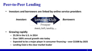
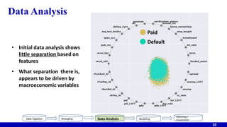
Forecasting
Peer-to-Peer
Lending Risk
Archange Giscard Destine
Steven Lerner
Erblin Mehmetaj
Hetal Shah
September 10, 2016
Forbes
Peer-to-Peer Lending
2
• Investors and borrowers are linked by online service providers
Investors Borrowers
• Growing rapidly
– $5.5B in the U.S. in 2014
– Over 100% annual growth rate today
– Expected to be a major player in consumer financing – over $150B by 2025
– Lending Club is the clear market leader
How Does It Work?
Borrowers
• Unsecured loan
• Rates often below
credit cards
• Done online –
quick and easy
3
Investors
• Higher rates, from
4 to 25+%
• Ability to spread
risk – invest as
little as $25 per
loan
Lending Club
• Collect ~ 5% fee up
front
• Collect ~ 1% on all
loan payments
• Pursue collections
But, roughly 14% of loans end in default
and
All risk is assumed by the investor
Objectives
Current
Develop a tool to help
investors avoid loans likely
to default
A model to forecast
probability of default, given
loan information …
emphasize default recall
versus precision
4
Future Work
For investors interested in taking
more risk, develop a tool to
determine effective interest rate
A model forecasting impact of
default (x, fraction of loan value)
Effective interest rate (z) =
n√[(1+i)n - p*x]
where i = original interest
n = loan duration, yrs
p = probability of default
12%
0%
Over 36 quarters
Unemployment rate
Charge-off rate
What’s Different Than Prior Work
• Lending Club’s new historical data set increases modeling difficulty
• Other studies ignored macroeconomic features … which are
important
5
Unsecured Personal Loan Delinquencies,2Q16 Unemployment Rate and Charge Off Rate
1.3% 7.7% TransUnion
Data Selection
• Loan data on completed loans from the Lending Club website
• Macroeconomic data
6
Measure State Fed. Value Slope* Reflection of:
Unemployment X X X Job loss & replacement difficulty
GDP X X X Overall economic activity
Disposable income X X X Cost/wage pressure
10-yr to 3-m T-bill spread X X Future economic growth
3-yr T-bill rate X X Short term inflation
Credit card rate (average) X X Alternative borrowing costs
* Slope is for 12 months prior, based on expert input
Data Ingestion: Sources
• Loan data: Lending Club website
– 111 features for each loan
– Historical data since June 2007
• Macroeconomic data
– Federal Reserve
– Bureau of Economic Analysis
– Bureau of Labor Statistics
– Cardhub
– National Conference of State Legislatures
• Collected data stored in data archive (PostgreSQL DB)
7
Data
Ingestion
Wrangling Computation / Analysis Modeling
Reporting /
Visualization
• Initial data reduction
– 111 historical features  29 features provided to investors
– Date range reduction to completed loans
• Data verification and cleanup
– Verify loan uniqueness
– Eliminate redundant data
– Eliminate non-informative features
(URL’s, free form, extremely sparse data, etc.)
– Trim entries: “months”, “%”, “+”, “years”, etc.
– Verify geographic scope
– Select uniform date structure for analysis and merging
– Address data that is both numeric and categorical
Data Wrangling… a big time consumer
8
Data Ingestion Wrangling Computation / Analysis Modeling
Reporting /
Visualization
220K instances
111 features
• Address all NaN entries
• Analyze outliers
• Economic calculations
– Least square slopes
– Interpolating for quarterly and annual
data
• Wrangle economic data: trimming
entries and using consistent format
• Merge economic and loan data
Data Wrangling (cont’d)
9
Categorical and
numerical wrangled
data frames
Surprise learning:
LC only verifies data for 31% of loans!
Data Ingestion Wrangling Computation / Analysis Modeling
Reporting /
Visualization
84K instances
30 features
- 21 loan
- 9 economic
Data Analysis
10
• Initial data analysis shows
little separation based on
features
• What separation there is,
appears to be driven by
macroeconomic variables
Data Ingestion Wrangling Data Analysis Modeling
Reporting /
Visualization
Paid
Default
Data Analysis (cont’d)
11
Features initially deemed important, showed little differentiation
Data Ingestion Wrangling Data Analysis Modeling
Reporting /
Visualization
Default
Paid
Overlap
Modeling
• Tested several modeling algorithms
– Logistical Regression
– Random Forest
– Naïve Bayes (Bernoulli, Gaussian, Multinomial)
– K-Nearest Neighbors
– Gradient Boosting
– Voting Classifier
• Manual feature exploration
• Created pipeline
– Standardization
– Feature reduction via PCA and LDA
12
Data Ingestion Wrangling Data Analysis Modeling
Reporting /
Visualization
Best recall was
0.58 to 0.62 …
was imbalanced
data the issue?
Modeling (cont’d)
13
-0.8
-0.6
-0.4
-0.2
0
0.2
0.4
0.6
Annual income
Feature importance for random forest
Data Ingestion Wrangling Data Analysis Modeling
Reporting /
Visualization
Feature importance for logistic regression
Annual income
Modeling (cont’d.)
• Balanced data set via undersampling paid loans
– Little improvement
– Losing lots of instances
• Added hyper-parameter tuning using GridSearch …
little improvement
• Balanced data via oversampling defaulted loans
– Extracted representative data sample (85/15, paid/default)
– Multiply remaining defaults 6X
– Train model using 80/20 split
– Final test versus extracted (unseen) data
14
Data Ingestion Wrangling Data Analysis Modeling
Reporting /
Visualization
De minimis
improvements
Modeling (cont’d)
• Sought expert advice
– Financial experts
– Modeling experts
• Adjusted feature set
– More responsive economic input
• 36/60 month lagging slopes  12 month leading slopes
• 36/60 month averages  point values
– Added critical ratios and indices to expand feature set
• Tested binary encoding
15
Data Ingestion Wrangling Data Analysis Modeling
Reporting /
Visualization
De minimis
improvements
Made a strategic
decision to modify
class weight to
enhance default
recall at the
expense of default
precision
Modeling: Metrics
Targeted 90+% default recall and 90+% paid precision
• Default recall
Defaults identified / total defaults
• Paid precision
Paids identified correctly / total instances identified as paid
16
Data Ingestion Wrangling Data Analysis Modeling
Reporting /
Visualization
Modeling (cont’d)
17
Logistic Regression Precision Recall F1 Score Support
Default (weight = 0.7) 0.52 0.94 0.67 13,568
Paid (weight = 0.3) 0.77 0.20 0.31 14,547
Unseen / Imbalanced Results
Default 0.16 0.97 0.20 115
Paid 0.97 0.18 0.30 734
Random Forest
Default (weight = 0.6) 0.53 0.92 0.68 13,568
Paid (weight = 0.4) 0.77 0.25 0.38 14,547
Unseen / Imbalanced Results
Default 0.16 0.95 0.28 115
Paid 0.97 0.24 0.39 734
What does
default recall = 0.97
and
default precision = 0.16
look like?
Data Ingestion Wrangling Data Analysis Modeling
Reporting /
Visualization
Reporting
• Tool (online) to predict loan status and probability of default
– Investor enters loan info
– Tool fetches macroeconomic data
– Above data is passed to webservice, which executes model and returns
predicted loan status and probability
• Tool developed using
– Flask interface with machine learning model as a RESTful webservice
– Jinja2 template
– HTML/CSS
– Javascript
18
Data Ingestion Wrangling Data Analysis Modeling Reporting
Demo
19
Conclusions
• Model effectively sequesters loans likely to default (97% default recall)
• Model cherry-picks loans not likely to default (97% paid precision)
• Achieving the above required class weighting which drives default recall
at the expense of default precision
… potentially good loans are misclassified as default
• Root causes appear to be lack of data separation, lack of feature
relevancy and imbalanced data
20
Future Work
Project specific
• Can we maintain recall and drive up precision by using logistic regression on
the total dataset followed by random forest on potential defaults?
• Can we identify or create more relevant features?
• Can we develop a tool for aggressive investors, providing impact of default?
General opportunity space around highly imbalanced data
21
21 21
Logistic Regression Random Forest
The authors would like to recognize the open source software that made this work possible
22
Questions?
Archange Giscard Destine ad1373@georgetown.edu Steven Lerner sll93@georgetown.edu
Erblin Mehmetaj em1109@georgetown.edu Hetal Shah hrs41@georgetown.edu

Forecasting peer to_peer_lending_risk

  • 1.
    Forecasting Peer-to-Peer Lending Risk Archange GiscardDestine Steven Lerner Erblin Mehmetaj Hetal Shah September 10, 2016 Forbes
  • 2.
    Peer-to-Peer Lending 2 • Investorsand borrowers are linked by online service providers Investors Borrowers • Growing rapidly – $5.5B in the U.S. in 2014 – Over 100% annual growth rate today – Expected to be a major player in consumer financing – over $150B by 2025 – Lending Club is the clear market leader
  • 3.
    How Does ItWork? Borrowers • Unsecured loan • Rates often below credit cards • Done online – quick and easy 3 Investors • Higher rates, from 4 to 25+% • Ability to spread risk – invest as little as $25 per loan Lending Club • Collect ~ 5% fee up front • Collect ~ 1% on all loan payments • Pursue collections But, roughly 14% of loans end in default and All risk is assumed by the investor
  • 4.
    Objectives Current Develop a toolto help investors avoid loans likely to default A model to forecast probability of default, given loan information … emphasize default recall versus precision 4 Future Work For investors interested in taking more risk, develop a tool to determine effective interest rate A model forecasting impact of default (x, fraction of loan value) Effective interest rate (z) = n√[(1+i)n - p*x] where i = original interest n = loan duration, yrs p = probability of default
  • 5.
    12% 0% Over 36 quarters Unemploymentrate Charge-off rate What’s Different Than Prior Work • Lending Club’s new historical data set increases modeling difficulty • Other studies ignored macroeconomic features … which are important 5 Unsecured Personal Loan Delinquencies,2Q16 Unemployment Rate and Charge Off Rate 1.3% 7.7% TransUnion
  • 6.
    Data Selection • Loandata on completed loans from the Lending Club website • Macroeconomic data 6 Measure State Fed. Value Slope* Reflection of: Unemployment X X X Job loss & replacement difficulty GDP X X X Overall economic activity Disposable income X X X Cost/wage pressure 10-yr to 3-m T-bill spread X X Future economic growth 3-yr T-bill rate X X Short term inflation Credit card rate (average) X X Alternative borrowing costs * Slope is for 12 months prior, based on expert input
  • 7.
    Data Ingestion: Sources •Loan data: Lending Club website – 111 features for each loan – Historical data since June 2007 • Macroeconomic data – Federal Reserve – Bureau of Economic Analysis – Bureau of Labor Statistics – Cardhub – National Conference of State Legislatures • Collected data stored in data archive (PostgreSQL DB) 7 Data Ingestion Wrangling Computation / Analysis Modeling Reporting / Visualization
  • 8.
    • Initial datareduction – 111 historical features  29 features provided to investors – Date range reduction to completed loans • Data verification and cleanup – Verify loan uniqueness – Eliminate redundant data – Eliminate non-informative features (URL’s, free form, extremely sparse data, etc.) – Trim entries: “months”, “%”, “+”, “years”, etc. – Verify geographic scope – Select uniform date structure for analysis and merging – Address data that is both numeric and categorical Data Wrangling… a big time consumer 8 Data Ingestion Wrangling Computation / Analysis Modeling Reporting / Visualization 220K instances 111 features
  • 9.
    • Address allNaN entries • Analyze outliers • Economic calculations – Least square slopes – Interpolating for quarterly and annual data • Wrangle economic data: trimming entries and using consistent format • Merge economic and loan data Data Wrangling (cont’d) 9 Categorical and numerical wrangled data frames Surprise learning: LC only verifies data for 31% of loans! Data Ingestion Wrangling Computation / Analysis Modeling Reporting / Visualization 84K instances 30 features - 21 loan - 9 economic
  • 10.
    Data Analysis 10 • Initialdata analysis shows little separation based on features • What separation there is, appears to be driven by macroeconomic variables Data Ingestion Wrangling Data Analysis Modeling Reporting / Visualization Paid Default
  • 11.
    Data Analysis (cont’d) 11 Featuresinitially deemed important, showed little differentiation Data Ingestion Wrangling Data Analysis Modeling Reporting / Visualization Default Paid Overlap
  • 12.
    Modeling • Tested severalmodeling algorithms – Logistical Regression – Random Forest – Naïve Bayes (Bernoulli, Gaussian, Multinomial) – K-Nearest Neighbors – Gradient Boosting – Voting Classifier • Manual feature exploration • Created pipeline – Standardization – Feature reduction via PCA and LDA 12 Data Ingestion Wrangling Data Analysis Modeling Reporting / Visualization Best recall was 0.58 to 0.62 … was imbalanced data the issue?
  • 13.
    Modeling (cont’d) 13 -0.8 -0.6 -0.4 -0.2 0 0.2 0.4 0.6 Annual income Featureimportance for random forest Data Ingestion Wrangling Data Analysis Modeling Reporting / Visualization Feature importance for logistic regression Annual income
  • 14.
    Modeling (cont’d.) • Balanceddata set via undersampling paid loans – Little improvement – Losing lots of instances • Added hyper-parameter tuning using GridSearch … little improvement • Balanced data via oversampling defaulted loans – Extracted representative data sample (85/15, paid/default) – Multiply remaining defaults 6X – Train model using 80/20 split – Final test versus extracted (unseen) data 14 Data Ingestion Wrangling Data Analysis Modeling Reporting / Visualization De minimis improvements
  • 15.
    Modeling (cont’d) • Soughtexpert advice – Financial experts – Modeling experts • Adjusted feature set – More responsive economic input • 36/60 month lagging slopes  12 month leading slopes • 36/60 month averages  point values – Added critical ratios and indices to expand feature set • Tested binary encoding 15 Data Ingestion Wrangling Data Analysis Modeling Reporting / Visualization De minimis improvements Made a strategic decision to modify class weight to enhance default recall at the expense of default precision
  • 16.
    Modeling: Metrics Targeted 90+%default recall and 90+% paid precision • Default recall Defaults identified / total defaults • Paid precision Paids identified correctly / total instances identified as paid 16 Data Ingestion Wrangling Data Analysis Modeling Reporting / Visualization
  • 17.
    Modeling (cont’d) 17 Logistic RegressionPrecision Recall F1 Score Support Default (weight = 0.7) 0.52 0.94 0.67 13,568 Paid (weight = 0.3) 0.77 0.20 0.31 14,547 Unseen / Imbalanced Results Default 0.16 0.97 0.20 115 Paid 0.97 0.18 0.30 734 Random Forest Default (weight = 0.6) 0.53 0.92 0.68 13,568 Paid (weight = 0.4) 0.77 0.25 0.38 14,547 Unseen / Imbalanced Results Default 0.16 0.95 0.28 115 Paid 0.97 0.24 0.39 734 What does default recall = 0.97 and default precision = 0.16 look like? Data Ingestion Wrangling Data Analysis Modeling Reporting / Visualization
  • 18.
    Reporting • Tool (online)to predict loan status and probability of default – Investor enters loan info – Tool fetches macroeconomic data – Above data is passed to webservice, which executes model and returns predicted loan status and probability • Tool developed using – Flask interface with machine learning model as a RESTful webservice – Jinja2 template – HTML/CSS – Javascript 18 Data Ingestion Wrangling Data Analysis Modeling Reporting
  • 19.
  • 20.
    Conclusions • Model effectivelysequesters loans likely to default (97% default recall) • Model cherry-picks loans not likely to default (97% paid precision) • Achieving the above required class weighting which drives default recall at the expense of default precision … potentially good loans are misclassified as default • Root causes appear to be lack of data separation, lack of feature relevancy and imbalanced data 20
  • 21.
    Future Work Project specific •Can we maintain recall and drive up precision by using logistic regression on the total dataset followed by random forest on potential defaults? • Can we identify or create more relevant features? • Can we develop a tool for aggressive investors, providing impact of default? General opportunity space around highly imbalanced data 21 21 21 Logistic Regression Random Forest
  • 22.
    The authors wouldlike to recognize the open source software that made this work possible 22 Questions? Archange Giscard Destine ad1373@georgetown.edu Steven Lerner sll93@georgetown.edu Erblin Mehmetaj em1109@georgetown.edu Hetal Shah hrs41@georgetown.edu