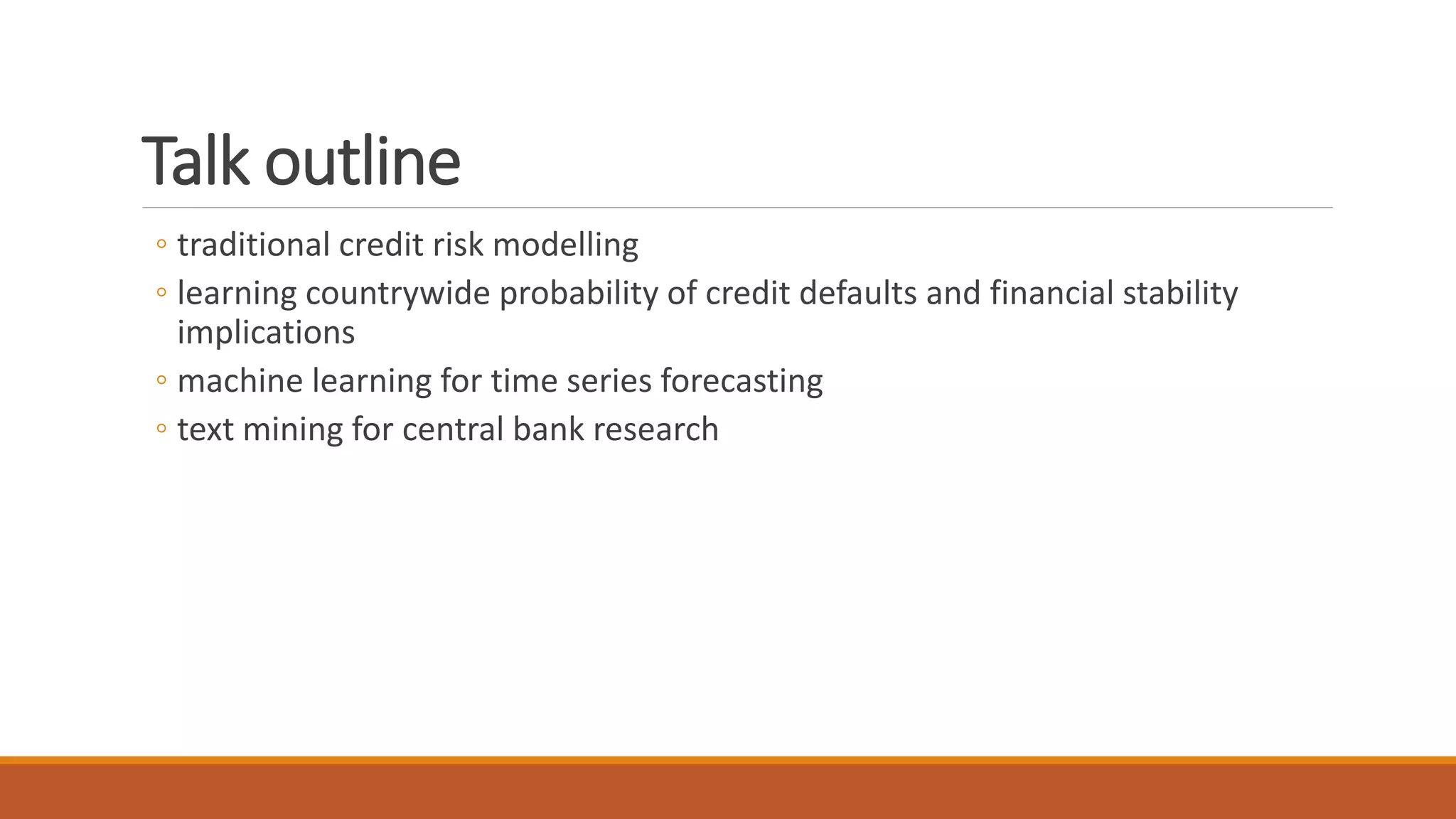
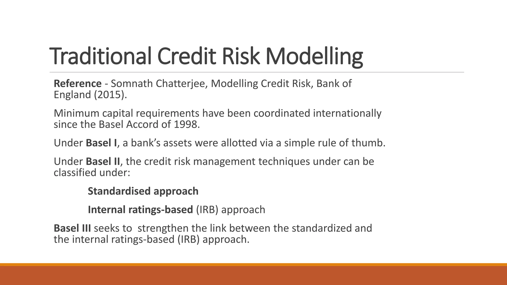
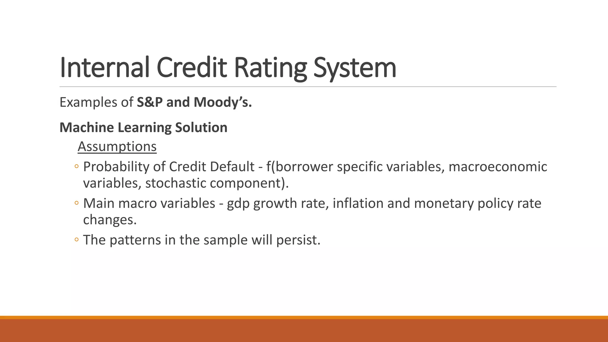
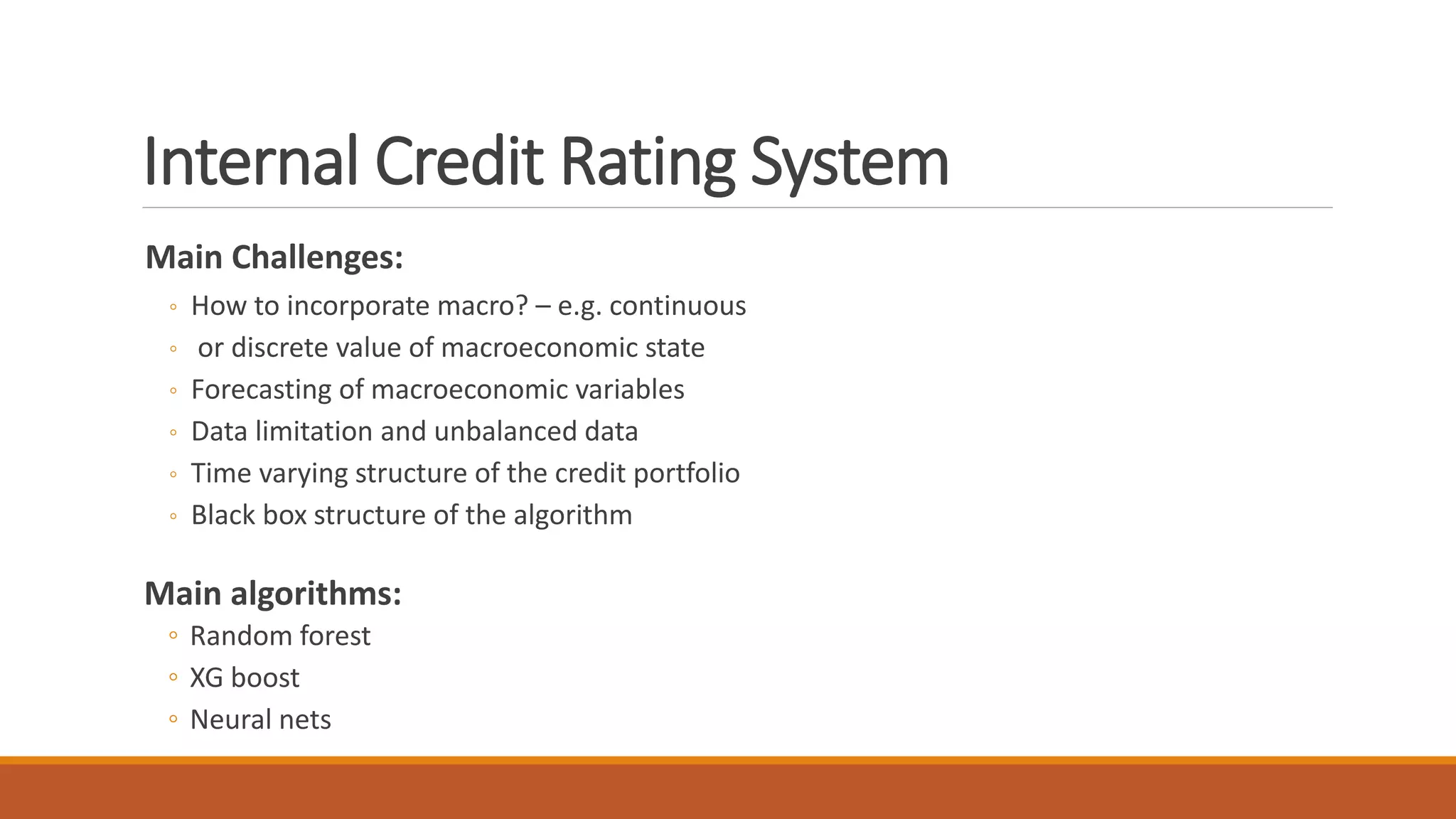
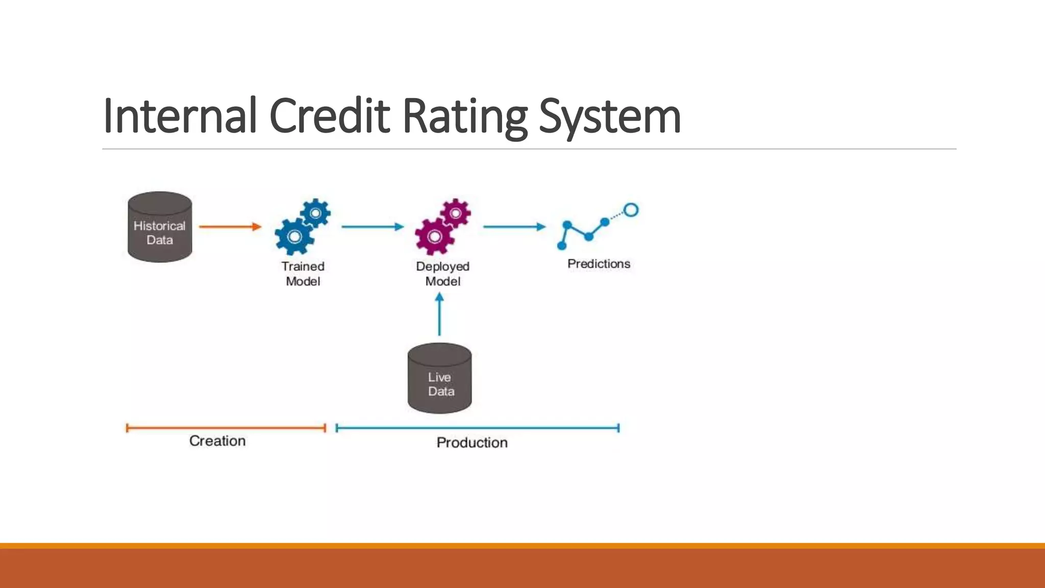
Machine learning algorithms can be used in various areas of banking and central banking. Specifically: 1) Traditional credit risk modeling can be enhanced with machine learning to predict probability of credit defaults based on borrower and macroeconomic variables. 2) Central banks can use credit bureau data and machine learning to monitor credit quality in real-time and provide recommendations to commercial banks. 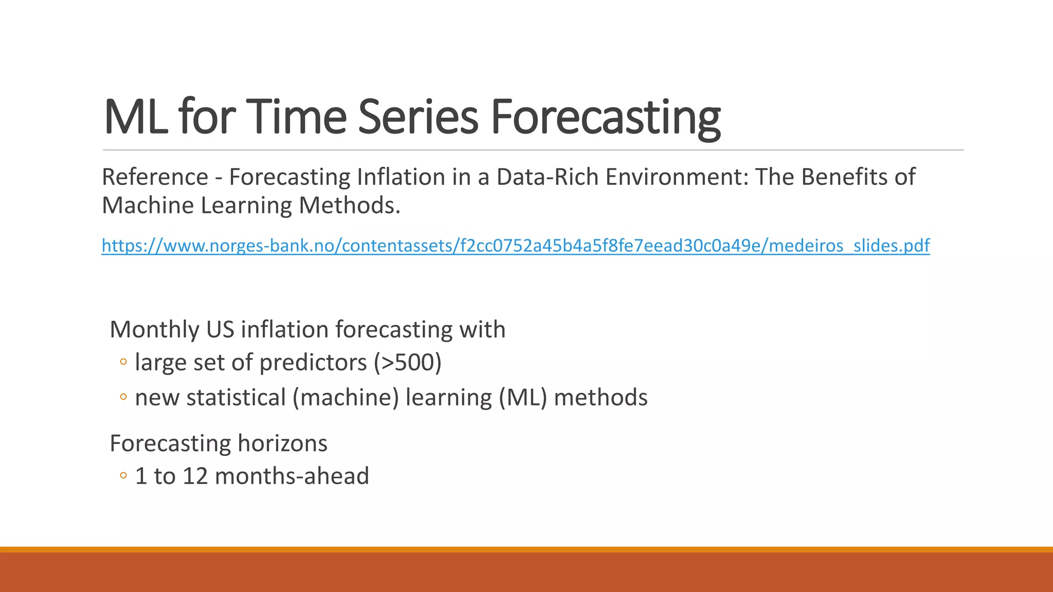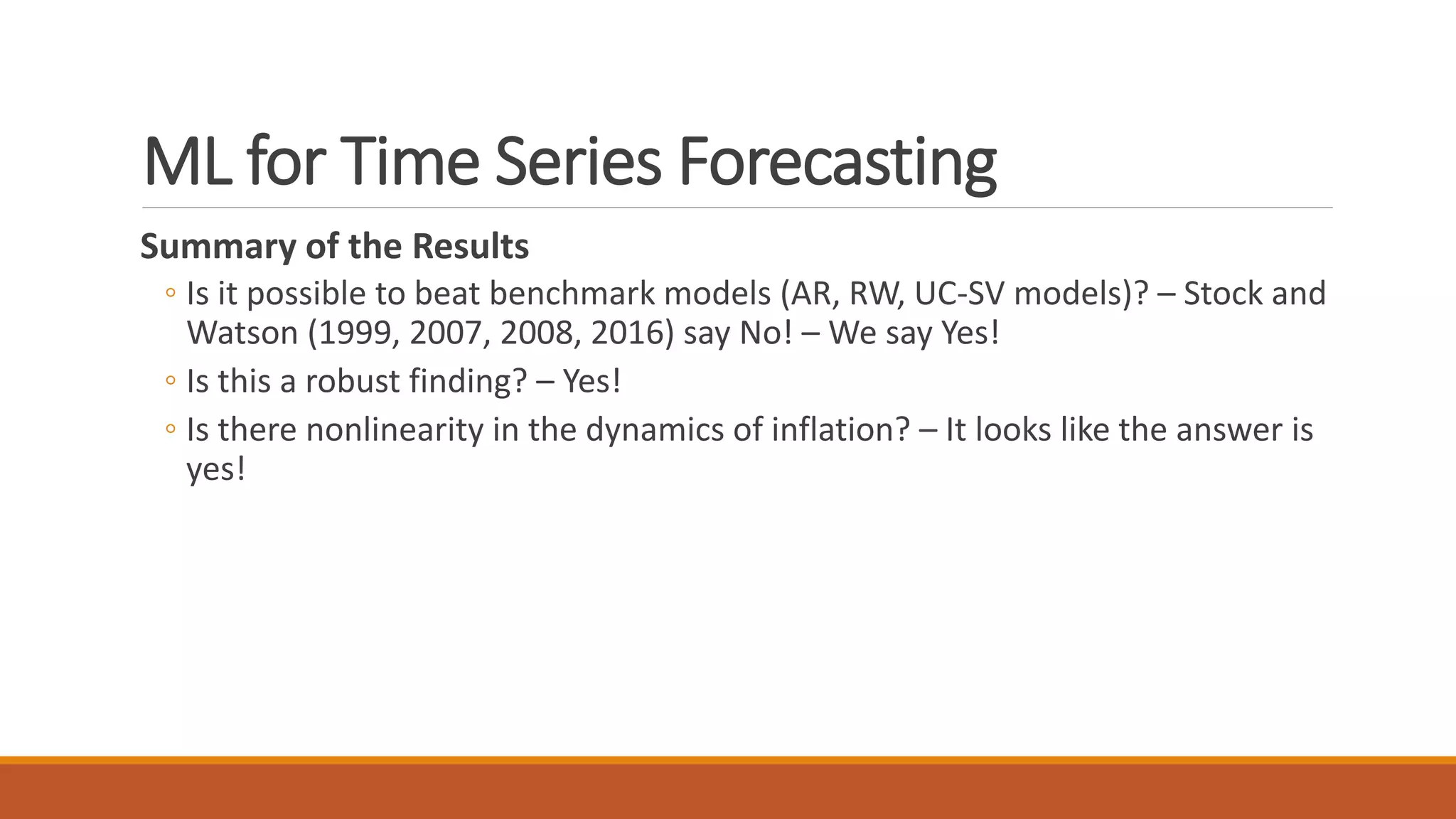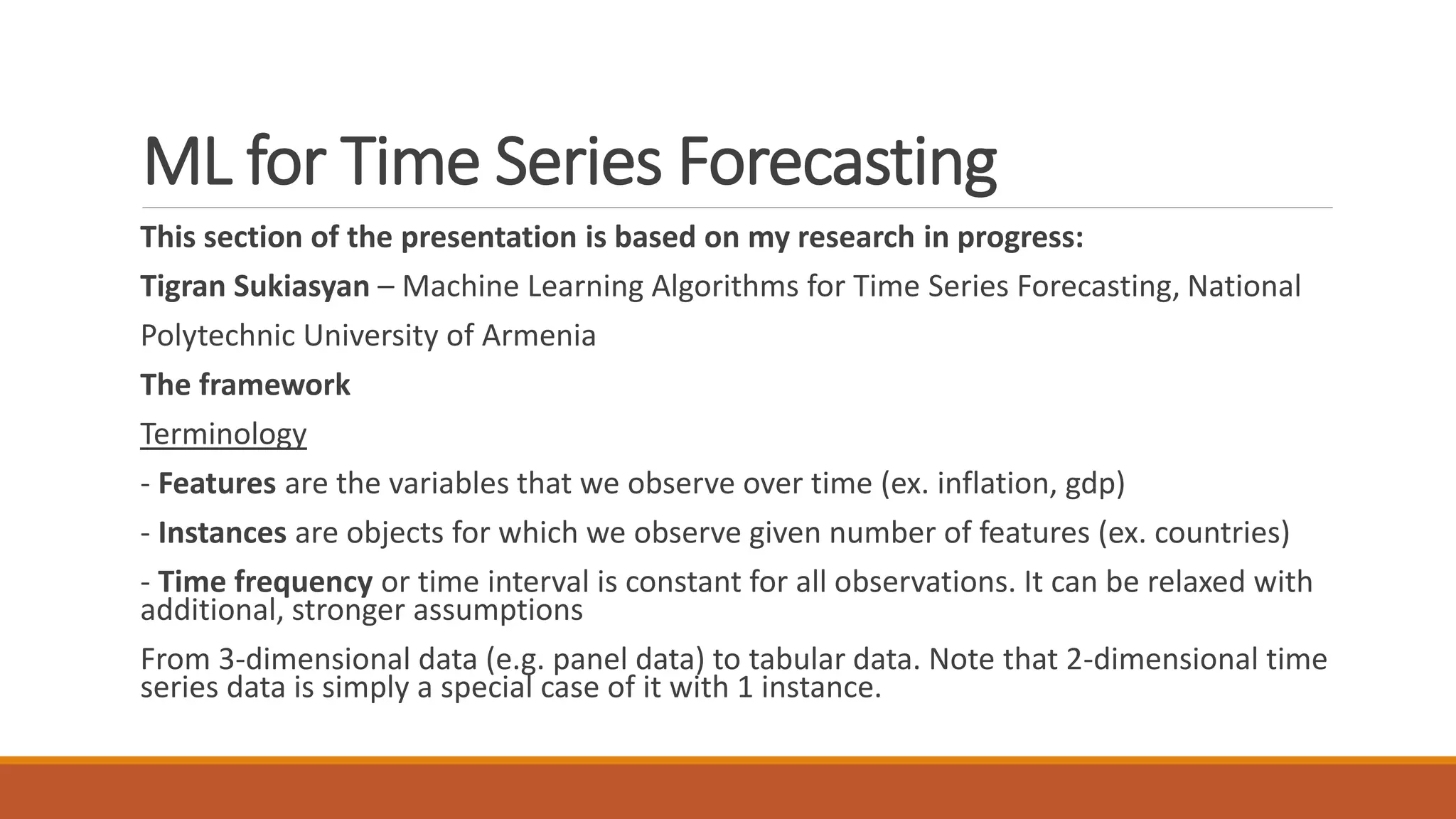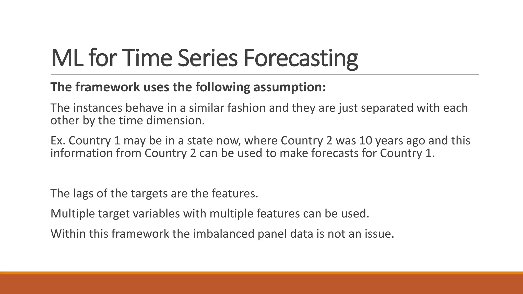3) Machine learning methods like random forests and neural networks outperform traditional models in time series forecasting of macroeconomic variables like inflation. 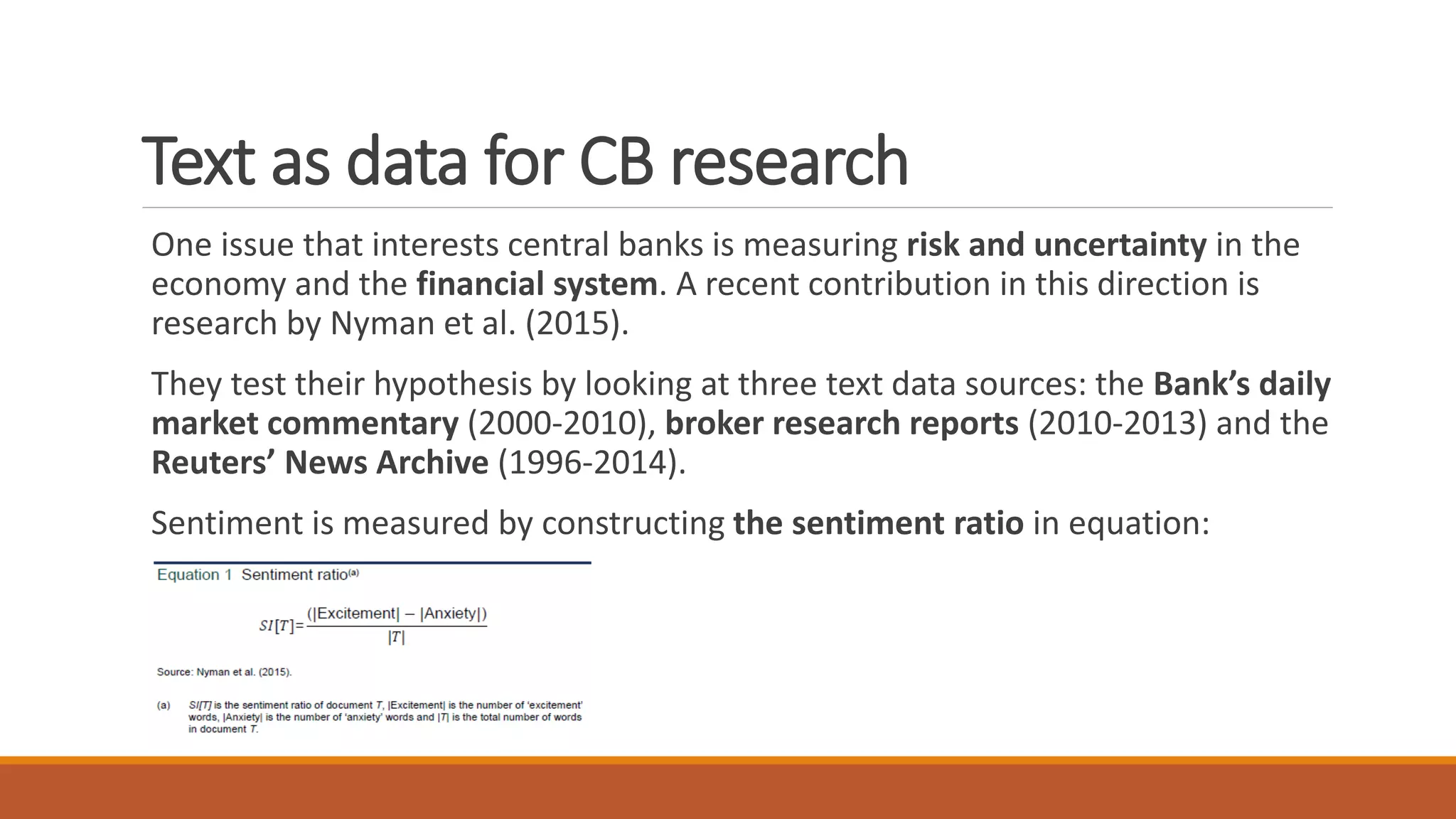4) Unstructured text and narrative data from news, market commentary, and reports can be analyzed with machine learning to measure economic sentiment, risk, uncertainty and consensus.

1. MACHINE LEARNING IN
BANKING
TIGRAN SUKIASYAN, PHD
DATA SCIENTIST AT AMERIABANK CJSC
VISITING LECTURER AT YEREVAN STATE UNIVERSITY - FACULTY OF MATHEMATICS AND
MECHANICS
URL: HTTP://WWW.LINKEDIN.COM/IN/TIGRAN -SUKIASYAN

2. Talk outline
◦ traditional credit risk modelling
◦ learning countrywide probability of credit defaults and financial stability
implications
◦ machine learning for time series forecasting
◦ text mining for central bank research

3. Christine Lagard’s speech
Central Banking and Fintech—A Brave New World?
“In 2040, the governor walking into the Bank will be of flesh and bones, and
behind the front door she will find people – at least a few,” Lagarde predicted.
https://www.imf.org/external/mmedia/view.aspx?vid=5595522478001
watch from 18:45 to 24:10.

4. HOW THE SYSTEM WORKS
The objective function of commercial banks
max Profit(X, ECL),
where X is a vector of variables related to the revenue
making (e.g. the availability of funds)
and ECL is the expected credit loss for the approved
credit portfolio.
Banking
&
Finance
Com.
Banks
Central
Banks
Consulting
& Audit
Services
IMF, BIS

5. Traditional Credit Risk Modelling
Reference - Somnath Chatterjee, Modelling Credit Risk, Bank of
England (2015).
Minimum capital requirements have been coordinated internationally
since the Basel Accord of 1998.
Under Basel I, a bank’s assets were allotted via a simple rule of thumb.
Under Basel II, the credit risk management techniques under can be
classified under:
Standardised approach
Internal ratings-based (IRB) approach
Basel III seeks to strengthen the link between the standardized and
the internal ratings-based (IRB) approach.

6. Traditional Credit Risk Modelling

7. Traditional Credit Risk Modelling
The expected loss of a portfolio is assumed to be equal to the proportion of obligors
that might default within a given time frame, multiplied by the outstanding exposure at
default, and once more by the loss given default, which represents the proportion of
the exposure that will not be recovered after default.
But the theoretical basis for calculating UL under the Basel II IRB framework stems from
the Vasicek (2002) loan portfolio value model.
Where S and Z are respectively the systematic and the idiosyncratic component and it
can be proved that rho is the asset correlation between two different obligors.

8. Traditional Credit Risk Modelling
The Vasicek model uses three inputs to calculate the probability of default (PD)
of an asset class. One input is the through-the-cycle PD (TTC_PD) specific for
that class. Further inputs are a portfolio common factor, such as an economic
index over the interval (0,T) given by S. The third input is the asset correlation.
A simple threshold condition determines whether the obligor i defaults or not.

9. Internal Credit Rating System
Examples of S&P and Moody’s.
Machine Learning Solution
Assumptions
◦ Probability of Credit Default - f(borrower specific variables, macroeconomic
variables, stochastic component).
◦ Main macro variables - gdp growth rate, inflation and monetary policy rate
changes.
◦ The patterns in the sample will persist.

10. Internal Credit Rating System
Main algorithms:
◦ Random forest
◦ XG boost
◦ Neural nets
Main Challenges:
◦ How to incorporate macro? – e.g. continuous
◦ or discrete value of macroeconomic state
◦ Forecasting of macroeconomic variables
◦ Data limitation and unbalanced data
◦ Time varying structure of the credit portfolio
◦ Black box structure of the algorithm

11. Internal Credit Rating System

12. Central Banks and Financial Stability
Credit bureau data (covers all the system)
Consolidation with forecasts of MP department
Real time monitoring of credit quality
Trained algorithm as a recommendation to commercial banks (can be an
important factor for potential entrant banks, too)

13. ML for Time Series Forecasting
Reference - Forecasting Inflation in a Data-Rich Environment: The Benefits of
Machine Learning Methods.
https://www.norges-bank.no/contentassets/f2cc0752a45b4a5f8fe7eead30c0a49e/medeiros_slides.pdf
Monthly US inflation forecasting with
◦ large set of predictors (>500)
◦ new statistical (machine) learning (ML) methods
Forecasting horizons
◦ 1 to 12 months-ahead

14. ML for Time Series Forecasting
Summary of the Results
◦ Is it possible to beat benchmark models (AR, RW, UC-SV models)? – Stock and
Watson (1999, 2007, 2008, 2016) say No! – We say Yes!
◦ Is this a robust finding? – Yes!
◦ Is there nonlinearity in the dynamics of inflation? – It looks like the answer is
yes!

15. What is policymaking? – From taking umbrella when it rains (no need to understand
why it rains) to changing the interest rates when shocks hit the economy (there is need
to understand the interconnectedness of shocks with the policy instrument in order to
respond accordingly).
Causality analysis with econometric tools sounds good, but the inference biases should
be considered:
- the framework of the assumptions about the data generation process
- sample representativeness, especially with time series data
Prediction with machine learning algorithms:
- Capture the non-linear patterns well, provide better predictions
- May be black box models that are hard to communicate
Econometrics vs Machine Learning for
Policymaking

16. This section of the presentation is based on my research in progress:
Tigran Sukiasyan – Machine Learning Algorithms for Time Series Forecasting, National
Polytechnic University of Armenia
The framework
Terminology
- Features are the variables that we observe over time (ex. inflation, gdp)
- Instances are objects for which we observe given number of features (ex. countries)
- Time frequency or time interval is constant for all observations. It can be relaxed with
additional, stronger assumptions
From 3-dimensional data (e.g. panel data) to tabular data. Note that 2-dimensional time
series data is simply a special case of it with 1 instance.
ML for Time Series Forecasting

17. The framework uses the following assumption:
The instances behave in a similar fashion and they are just separated with each
other by the time dimension.
Ex. Country 1 may be in a state now, where Country 2 was 10 years ago and this
information from Country 2 can be used to make forecasts for Country 1.
The lags of the targets are the features.
Multiple target variables with multiple features can be used.
Within this framework the imbalanced panel data is not an issue.
ML for Time Series Forecasting

18. ML for Time Series Forecasting
Dataset Date Feature 1
(m-i)-th
lag)
Feature 1
(m-th lag)
Feature 2
(n-j)-th lag)
Feature 2
(n-th lag)
Target
Instance 1 Period 1
Period 2
Period 3
Instance 2 Period 1
Period 2
Period 3
Instance 3 Period 1
Period 2
Period 3
ML ALGORITHM
HYPERPARAMETER
TUNING

19. INITIAL RESULTS FOR US INFLATION
Here are the semester ahead
forecasts of a machine
learning algorithm that uses
from 6th to 12th lags of the
inflation rate (blue line),
a benchmark model that uses
the simple average of the
same lags (dashed line),
and the actual inflation
(green line).
MSE_ML = 0.03
MSE_benchmark = 0.05
-0.4
-0.2
0
0.2
0.4
0.6
0.8
Jun2015
Jul2015
Aug2015
Sep2015
Oct2015
Nov2015
Dec2015
Jan2016
Feb2016
Mar2016
Apr2016
May2016
Jun2016
Jul2016
Aug2016
Sep2016
Oct2016
Nov2016
Dec2016
Jan2017
Feb2017
Mar2017
Apr2017
May2017
Jun2017
Jul2017
Aug2017
Sep2017
Oct2017
Nov2017
Dec2017
Jan2018
Feb2018
Mar2018
Apr2018
May2018
US MoM Inflation
Actual_inflation Benchmark_forecast ML_forecast

20. Future work:
◦ How to deal with seasonality?
◦ How to deal with non stationarity?
◦ How to choose the right lags?
◦ How to do cross validation?
◦ How to interpret the results (if possible)?
◦ Other?
Econometrics vs Machine Learning for
Policymaking

21. Reference – Text Mining For Central Banks,
David Bholat, Stephen Hansen, Pedro Santos
and Cheryl Schonhardt-Bailey.
McLaren and Shanbhogue (2011) offer a fine
example of what can be done. Using Google
data on search volumes, they find that such
data provides a timelier tracking of key
economic variables than do official statistics.
Google searches for Jobseeker’s Allowance
closely track official unemployment.
Text as data for CB research

22. Text as data for CB research
One issue that interests central banks is measuring risk and uncertainty in the
economy and the financial system. A recent contribution in this direction is
research by Nyman et al. (2015).
They test their hypothesis by looking at three text data sources: the Bank’s daily
market commentary (2000-2010), broker research reports (2010-2013) and the
Reuters’ News Archive (1996-2014).
Sentiment is measured by constructing the sentiment ratio in equation:

23. Text as data for CB research
The sign of the ratio gives an indication of
market sentiment: bullish, if the ratio is
positive, or bearish, if the number is
negative.
In addition, they measure narrative
consensus. In particular, their approach is
to group articles into topic clusters. The
uncertainty in the distribution of topics
then acts as a proxy for uncertainty. In
other words, reduced entropy in the topic
distribution is used as an indicator of topic
concentration or consensus.

24. Thank You!