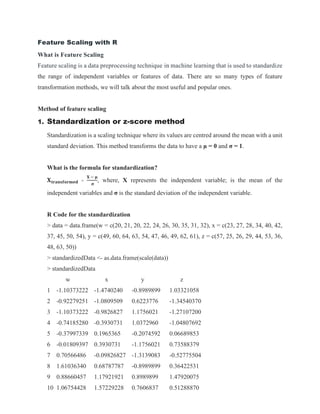
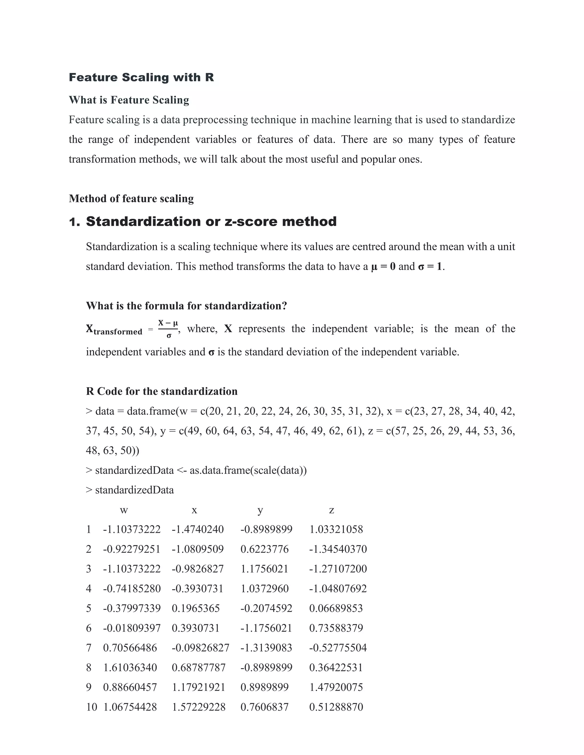
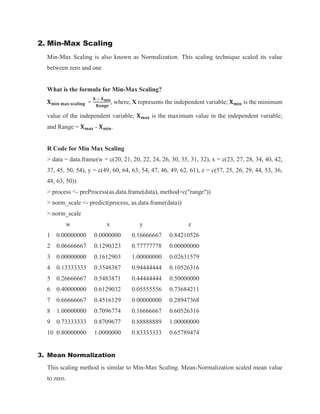
Feature scaling is a technique used in machine learning to standardize the range of independent variables or features of data. There are several common feature scaling methods including standardization, min-max scaling, and mean normalization. Standardization transforms the data to have a mean of 0 and standard deviation of 1. Min-max scaling scales features between 0 and 1. Mean normalization scales the mean value to zero. The document then provides the formulas and R code examples for implementing each of these scaling methods.

1. Feature Scaling with R
What is Feature Scaling
Feature scaling is a data preprocessing technique in machine learning that is used to standardize
the range of independent variables or features of data. There are so many types of feature
transformation methods, we will talk about the most useful and popular ones.
Method of feature scaling
1. Standardization or z-score method
Standardization is a scaling technique where its values are centred around the mean with a unit
standard deviation. This method transforms the data to have a µ = 0 and σ = 1.
What is the formula for standardization?
𝐗𝐭𝐫𝐚𝐧𝐬𝐟𝐨𝐫𝐦𝐞𝐝 =
𝐗 − 𝛍
𝛔
, where, X represents the independent variable; is the mean of the
independent variables and σ is the standard deviation of the independent variable.
R Code for the standardization
> data = data.frame(w = c(20, 21, 20, 22, 24, 26, 30, 35, 31, 32), x = c(23, 27, 28, 34, 40, 42,
37, 45, 50, 54), y = c(49, 60, 64, 63, 54, 47, 46, 49, 62, 61), z = c(57, 25, 26, 29, 44, 53, 36,
48, 63, 50))
> standardizedData <- as.data.frame(scale(data))
> standardizedData
w x y z
1 -1.10373222 -1.4740240 -0.8989899 1.03321058
2 -0.92279251 -1.0809509 0.6223776 -1.34540370
3 -1.10373222 -0.9826827 1.1756021 -1.27107200
4 -0.74185280 -0.3930731 1.0372960 -1.04807692
5 -0.37997339 0.1965365 -0.2074592 0.06689853
6 -0.01809397 0.3930731 -1.1756021 0.73588379
7 0.70566486 -0.09826827 -1.3139083 -0.52775504
8 1.61036340 0.68787787 -0.8989899 0.36422531
9 0.88660457 1.17921921 0.8989899 1.47920075
10 1.06754428 1.57229228 0.7606837 0.51288870

2. 2. Min-Max Scaling
Min-Max Scaling is also known as Normalization. This scaling technique scaled its value
between zero and one
What is the formula for Min-Max Scaling?
𝐗𝐦𝐢𝐧 𝐦𝐚𝐱 𝐬𝐜𝐚𝐥𝐢𝐧𝐠 =
𝐗 − 𝐗𝐦𝐢𝐧
𝐑𝐚𝐧𝐠𝐞
, where, X represents the independent variable; 𝐗𝐦𝐢𝐧 is the minimum
value of the independent variable; 𝐗𝐦𝐚𝐱 is the maximum value in the independent variable;
and Range = 𝐗𝐦𝐚𝐱 - 𝐗𝐦𝐢𝐧.
R Code for Min Max Scaling
> data = data.frame(w = c(20, 21, 20, 22, 24, 26, 30, 35, 31, 32), x = c(23, 27, 28, 34, 40, 42,
37, 45, 50, 54), y = c(49, 60, 64, 63, 54, 47, 46, 49, 62, 61), z = c(57, 25, 26, 29, 44, 53, 36,
48, 63, 50))
> process <- preProcess(as.data.frame(data), method=c("range"))
> norm_scale <- predict(process, as.data.frame(data))
> norm_scale
w x y z
1 0.00000000 0.0000000 0.16666667 0.84210526
2 0.06666667 0.1290323 0.77777778 0.00000000
3 0.00000000 0.1612903 1.00000000 0.02631579
4 0.13333333 0.3548387 0.94444444 0.10526316
5 0.26666667 0.5483871 0.44444444 0.50000000
6 0.40000000 0.6129032 0.05555556 0.73684211
7 0.66666667 0.4516129 0.00000000 0.28947368
8 1.00000000 0.7096774 0.16666667 0.60526316
9 0.73333333 0.8709677 0.88888889 1.00000000
10 0.80000000 1.0000000 0.83333333 0.65789474
3. Mean Normalization
This scaling method is similar to Min-Max Scaling. Mean-Normalization scaled mean value
to zero.

3. What is the formula for Mean Normalization?
𝐗𝐦𝐞𝐚𝐧 𝐧𝐨𝐫𝐦𝐚𝐥𝐢𝐳𝐚𝐭𝐢𝐨𝐧 =
𝐗 − 𝐗𝐦𝐞𝐚𝐧
𝐫𝐚𝐧𝐠𝐞
, where, X represents the independent variable; 𝐗𝐦𝐞𝐚𝐧 is the
mean of the independent variables or the dataset; and Range = 𝐗𝐦𝐚𝐱 - 𝐗𝐦𝐢𝐧.
R Code for Mean Normalization
> data = data.frame(w = c(20, 21, 20, 22, 24, 26, 30, 35, 31, 32), x = c(23, 27, 28, 34, 40, 42,
37, 45, 50, 54), y = c(49, 60, 64, 63, 54, 47, 46, 49, 62, 61), z = c(57, 25, 26, 29, 44, 53, 36,
48, 63, 50))
> datamean <- as.data.frame(sapply(data, function(x) (x-mean(x))/(max(x)-min(x))))
> datamean
w x y z
1 -0.406666667 -0.48387097 -0.36111111 0.36578947
2 -0.340000000 -0.35483871 0.25000000 -0.47631579
3 -0.406666667 -0.32258065 0.47222222 -0.45000000
4 -0.273333333 -0.12903226 0.41666667 -0.37105263
5 -0.140000000 0.06451613 -0.08333333 0.02368421
6 -0.006666667 0.12903226 -0.47222222 0.26052632
7 0.260000000 -0.03225806 -0.52777778 -0.18684211
8 0.593333333 0.22580645 -0.36111111 0.12894737
9 0.326666667 0.38709677 0.36111111 0.52368421
10 0.393333333 0.51612903 0.30555556 0.18157895
4. Max Absolute Scaling
this scaling method scaled each feature by its maximum absolute value.
What is the formula for Max Absolute Scaling?
Max absolute scaling =
𝐗
⌊⌊𝐗𝐦𝐚𝐱⌋⌋
where X represents the independent variable and ⌊𝐗𝐦𝐚𝐱⌋ is the
absolute value of the maximum value in the dataset

4. R Code for Max Absolute Scaling
> data = data.frame(w = c(20, 21, 20, 22, 24, 26, 30, 35, 31, 32), x = c(23, 27, 28, 34, 40, 42,
37, 45, 50, 54), y = c(49, 60, 64, 63, 54, 47, 46, 49, 62, 61), z = c(57, 25, 26, 29, 44, 53, 36,
48, 63, 50))
> maxAbsoluteScaling_w = data$w/max(data$w)
> maxAbsoluteScaling_x = data$x/max(data$x)
> maxAbsoluteScaling_y = data$y/max(data$y)
> maxAbsoluteScaling_z = data$z/max(data$z)
>maxAbsoluteScaling = data.frame('w' = maxAbsoluteScaling_w, 'x'=
maxAbsoluteScaling_x, 'y'= maxAbsoluteScaling_y, 'z'= maxAbsoluteScaling_z)
> maxAbsoluteScaling
>
w x y z
1 0.5714286 0.4259259 0.765625 0.9047619
2 0.6000000 0.5000000 0.937500 0.3968254
3 0.5714286 0.5185185 1.000000 0.4126984
4 0.6285714 0.6296296 0.984375 0.4603175
5 0.6857143 0.7407407 0.843750 0.6984127
6 0.7428571 0.7777778 0.734375 0.8412698
7 0.8571429 0.6851852 0.718750 0.5714286
8 1.0000000 0.8333333 0.765625 0.7619048
9 0.8857143 0.9259259 0.968750 1.0000000
10 0.9142857 1.0000000 0.953125 0.7936508
5. Robust Scaling
this scaling technique transforms the value to make the median = 0 and IQR = 1. This is used
when there are many outliers in the dataset.
What is the formula for Robust Scaling?
𝐗𝐫𝐨𝐛𝐮𝐬𝐭 𝐬𝐜𝐚𝐥𝐢𝐧𝐠 =
𝐗 − 𝐗𝐦𝐞𝐝𝐢𝐚𝐧
𝐈𝐐𝐑
, where, X represents the independent variable; 𝐗𝐦𝐞𝐝𝐢𝐚𝐧 is the
median of the independent variable; and IQR = 𝐐𝟑 - 𝐐1 that is the Inter Quarter Range of the
independent variable.

5. R Code for Robust Scaling
> data = data.frame(w = c(20, 21, 20, 22, 24, 26, 30, 35, 31, 32), x = c(23, 27, 28, 34, 40, 42,
37, 45, 50, 54), y = c(49, 60, 64, 63, 54, 47, 46, 49, 62, 61), z = c(57, 25, 26, 29, 44, 53, 36,
48, 63, 50))
> median_w = median(data$w)
> median_x = median(data$x)
> median_y = median(data$y)
> median_z = median(data$z)
> IQR_w = IQR(data$w)
> IQR_x = IQR(data$x)
> IQR_y = IQR(data$y)
> IQR_z = IQR(data$z)
> IQR_w = IQR(data$w)
> robustTransformed_w = (data$w - median_w)/IQR_w
> robustTransformed_x = (data$x - median_x)/IQR_x
> robustTransformed_y = (data$y - median_y)/IQR_y
> robustTransformed_z = (data$z - median_z)/IQR_z
> robustTransformed = data.frame('w' = (data$w - median_w)/IQR_w, 'x'= (data$x -
median_x)/IQR_x, 'y'= (data$y - median_y)/IQR_y, 'z'= (data$z - median_z)/IQR_z)
> robustTransformed
w x y
1 -0.5263158 -1.0508475 -0.6274510 0.51162791
2 -0.4210526 -0.7796610 0.2352941 -0.97674419
3 -0.5263158 -0.7118644 0.5490196 -0.93023256
4 -0.3157895 -0.3050847 0.4705882 -0.79069767
5 -0.1052632 0.1016949 -0.2352941 -0.09302326
6 0.1052632 0.2372881 -0.7843137 0.32558140
7 0.5263158 -0.1016949 -0.8627451 -0.46511628
8 1.0526316 0.4406780 -0.6274510 0.09302326
9 0.6315789 0.7796610 0.3921569 0.79069767
10 0.7368421 1.0508475 0.3137255 0.18604651

6. 6. Unit-Length Normalization
these are transformed by dividing each observation in the vector by the Euclidean length of the
vector.
What is the formula for the Unit Length Normalization?
𝐗𝐮𝐧𝐢𝐭−𝐥𝐞𝐧𝐠𝐭𝐡 𝐧𝐨𝐫𝐦 =
𝐗
‖𝐗‖
, where, X represents the independent variable or original data; ‖𝐗‖ is
the Euclidean distance of the vector.
R Code for Unit Length Normalization
data = data.frame(w = c(20, 21, 20, 22, 24, 26, 30, 35, 31, 32), x = c(23, 27, 28, 34, 40, 42, 37,
45, 50, 54), y = c(49, 60, 64, 63, 54, 47, 46, 49, 62, 61), z = c(57, 25, 26, 29, 44, 53, 36, 48,
63, 50))
> unitTransformed_w = data$w/sqrt(sum(data$w * data$w))
> unitTransformed_x = data$x/sqrt(sum(data$x * data$x))
> unitTransformed_y = data$y/sqrt(sum(data$y * data$y))
> unitTransformed_z = data$z/sqrt(sum(data$z * data$z))
>
> unitTransformed = data.frame('w' = unitTransformed_w, 'x' = unitTransformed_x, 'y' =
unitTransformed_y, 'z' = unitTransformed_z)
>
> unitTransformed
w x y z
1 0.2375739 0.1855080 0.2770839 0.4010010
2 0.2494526 0.2177703 0.3392864 0.1758776
3 0.2375739 0.2258358 0.3619055 0.1829127
4 0.2613313 0.2742292 0.3562507 0.2040180
5 0.2850887 0.3226226 0.3053578 0.3095446
6 0.3088461 0.3387537 0.2657744 0.3728606
7 0.3563609 0.2984259 0.2601196 0.2532638
8 0.4157544 0.3629504 0.2770839 0.3376850
9 0.3682396 0.4032783 0.3505960 0.4432116
10 0.3801183 0.4355405 0.3449412 0.3517552

7. 7. Logarithmic Transformations
these are more suitable means of transforming a highly skewed or kurtotic distribution of
continuous independent variables with non-linear relationships into a more normalized dataset.
How to perform the logarithmic transformation
The logarithmic transformation is performed by taking the logarithm function of the
independent variable. These are done naturally by taking the natural log(In) of each
observation in the distribution
R Code for logarithmic transformation
> data = data.frame(w = c(20, 21, 20, 22, 24, 26, 30, 35, 31, 32), x = c(23, 27, 28, 34, 40, 42,
37, 45, 50, 54), y = c(49, 60, 64, 63, 54, 47, 46, 49, 62, 61), z = c(57, 25, 26, 29, 44, 53, 36,
48, 63, 50))
>
> logTransformed = log10(data)
> logTransformed
w x y z
1 1.301030 1.361728 1.690196 1.755875
2 1.322219 1.431364 1.778151 1.397940
3 1.301030 1.447158 1.806180 1.414973
4 1.342423 1.531479 1.799341 1.462398
5 1.380211 1.602060 1.732394 1.643453
6 1.414973 1.623249 1.672098 1.724276
7 1.477121 1.568202 1.662758 1.556303
8 1.544068 1.653213 1.690196 1.681241
9 1.491362 1.698970 1.792392 1.799341
10 1.505150 1.732394 1.785330 1.698970
8. Reciprocal Transformations
The reciprocal transformation can only be applied to a non-zero dataset. It is suitable or
commonly used when distributions have skewed or clear outliers.

8. How to perform a reciprocal transformation
The reciprocal transformation is performed by taking the inverse function of the independent
variable. It is defined as
𝟏
𝐱
where x is the independent variable.
R Code for reciprocal transformation
> data = data.frame(w = c(20, 21, 20, 22, 24, 26, 30, 35, 31, 32), x = c(23, 27, 28, 34, 40, 42,
37, 45, 50, 54), y = c(49, 60, 64, 63, 54, 47, 46, 49, 62, 61), z = c(57, 25, 26, 29, 44, 53, 36,
48, 63, 50))
> reciprocalTransformed = (1/data)
> reciprocalTransformed
w x y z
1 0.05000000 0.04347826 0.02040816 0.01754386
2 0.04761905 0.03703704 0.01666667 0.04000000
3 0.05000000 0.03571429 0.01562500 0.03846154
4 0.04545455 0.02941176 0.01587302 0.03448276
5 0.04166667 0.02500000 0.01851852 0.02272727
6 0.03846154 0.02380952 0.02127660 0.01886792
7 0.03333333 0.02702703 0.02173913 0.02777778
8 0.02857143 0.02222222 0.02040816 0.02083333
9 0.03225806 0.02000000 0.01612903 0.01587302
10 0.03125000 0.01851852 0.01639344 0.02000000
9. Arcsine Transformation
The arcsine transformation is also known as the angular transformation or arcsine square root
transformation. This transformation is performed only when the variables range between 0 to
1 by taking the arcsine of the square root of the independent variable. Anytime a vector value
ranges outside 0 to 1, we need to convert each value to be in the range of 0 to 1 by
𝐗
𝐗𝐦𝐚𝐱
=
𝐗𝐜𝐨𝐧𝐯𝐞𝐫𝐭𝐞𝐝 then take the arcsine of the square root of the converted value by arcsine(square root
(𝐗𝐜𝐨𝐧𝐯𝐞𝐫𝐭𝐞𝐝)).

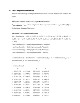
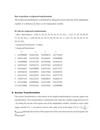
9. R Code for arcsine transformation
data = data.frame(w = c(20, 21, 20, 22, 24, 26, 30, 35, 31, 32), x = c(23, 27, 28, 34, 40, 42, 37,
45, 50, 54), y = c(49, 60, 64, 63, 54, 47, 46, 49, 62, 61), z = c(57, 25, 26, 29, 44, 53, 36, 48,
63, 50))
> arcsinemodified_w = data$w/max(data$w)
> arcsinemodified_x = data$x/max(data$x)
> arcsinemodified_y = data$y/max(data$y)
> arcsinemodified_z = data$z/max(data$z)
> arcsineTransformed_w = asin(sqrt(arcsinemodified_w))
> arcsineTransformed_x = asin(sqrt(arcsinemodified_x))
> arcsineTransformed_y = asin(sqrt(arcsinemodified_y))
> arcsineTransformed_z = asin(sqrt(arcsinemodified_z))
> arcsineTransformed = data.frame('w' = arcsineTransformed_w, 'x' = arcsineTransformed_x,
'y' = arcsineTransformed_y, 'z' = arcsineTransformed_z)
> arcsineTransformed
w x y z
1 0.8570719 0.7110504 1.065436 1.2570684
2 0.8860771 0.7853982 1.318116 0.6814770
3 0.8570719 0.8039209 1.570796 0.6976468
4 0.9154304 0.9165257 1.445468 0.7456738
5 0.9756718 1.0365703 1.164419 0.9894260
6 1.0389882 1.0799136 1.029336 1.1610142
7 1.1831996 0.9751020 1.011806 0.8570719
8 1.5707963 1.1502620 1.065436 1.0610566
9 1.2259397 1.2951535 1.393086 1.5707963
10 1.2736738 1.5707963 1.352562 1.0992586
10. Square Root Transformation
Square root transformation can be used as
[i] for data that follow a Poisson distribution or small whole numbers
[ii] usually works for data with non-constant variance
[iii] may also be appropriate for percentage data where the range is between 0 and 30% or

10. between 70 and 100%.
Square root transformation is considered to be weaker than logarithmic or cube root
transforms. This is done by taking the square of each data point.
How to perform a square root transformation
Square root transformation is performed by taking the square root function of the
independent variable. It is defined as √𝐱 where x is the independent variable.
R Code for square root transformation
> data = data.frame(w = c(20, 21, 20, 22, 24, 26, 30, 35, 31, 32), x = c(23, 27, 28, 34, 40,
42, 37, 45, 50, 54), y = c(49, 60, 64, 63, 54, 47, 46, 49, 62, 61), z = c(57, 25, 26, 29, 44,
53, 36, 48, 63, 50))
> sqrtTransformed = sqrt(data)
> sqrtTransformed
w x y z
1 4.472136 4.795832 7.000000 7.549834
2 4.582576 5.196152 7.745967 5.000000
3 4.472136 5.291503 8.000000 5.099020
4 4.690416 5.830952 7.937254 5.385165
5 4.898979 6.324555 7.348469 6.633250
6 5.099020 6.480741 6.855655 7.280110
7 5.477226 6.082763 6.782330 6.000000
8 5.916080 6.708204 7.000000 6.928203
9 5.567764 7.071068 7.874008 7.937254
10 5.656854 7.348469 7.810250 7.071068
11. Cube Root Transformations
The cube root transformation is useful for reducing right skewness of a distribution. This
transformation method can be applied to positive and negative values in a dataset.
How to perform a cube root transformation

11. The cube root transformation is performed by taking the inverse function of the
independent variable. It is defined as √𝐱
𝟑
or 𝐱𝟏 𝟑
⁄
where x is the independent variable.
R Code for cube root transformation
> data = data.frame(w = c(20, 21, 20, 22, 24, 26, 30, 35, 31, 32), x = c(23, 27, 28, 34, 40,
42, 37, 45, 50, 54), y = c(49, 60, 64, 63, 54, 47, 46, 49, 62, 61), z = c(57, 25, 26, 29, 44,
53, 36, 48, 63, 50))
> cubeTransformed = (data^(1/3))
> cubeTransformed
w x y z
1 2.714418 2.843867 3.659306 3.848501
2 2.758924 3.000000 3.914868 2.924018
3 2.714418 3.036589 4.000000 2.962496
4 2.802039 3.239612 3.979057 3.072317
5 2.884499 3.419952 3.779763 3.530348
6 2.962496 3.476027 3.608826 3.756286
7 3.107233 3.332222 3.583048 3.301927
8 3.271066 3.556893 3.659306 3.634241
9 3.141381 3.684031 3.957892 3.979057
10 3.174802 3.779763 3.936497 3.684031
12. Box-Cox Transformation
Box-Cox Transformation is a power transformation used to convert non-normal dependent
variables into a normal distribution is called the box-cox transformation and its input
dataset must only contain positive values. The Box-Cox transformation assist to confirm
whether the standard deviation is the smallest or not.
The mathematical formula for Box-cox transformation is x(λ) = {
𝐱𝛌 − 𝟏
𝛌
, 𝐢𝐟 𝛌 ≠ 𝟎;
𝐥𝐨𝐠 𝐱, 𝐢𝐟 𝛌 = 𝟎.
where,
λ is a parameter to be determined using the dataset
λ varies from -5 to 5

12. λ values are all considered and the optimal value for the dataset is selected which is the
best approximation of a normal distribution curve of the error terms.
R Code for Box-Cox Transformation
> data = data.frame(w = c(20, 21, 20, 22, 24, 26, 30, 35, 31, 32), x = c(23, 27, 28, 34, 40,
42, 37, 45, 50, 54), y = c(49, 60, 64, 63, 54, 47, 46, 49, 62, 61), z = c(57, 25, 26, 29, 44,
53, 36, 48, 63, 50))
> ts(data)
Time Series:
Start = 1
End = 10
Frequency = 1
w x y z
1 20 23 49 57
2 21 27 60 25
3 20 28 64 26
4 22 34 63 29
5 24 40 54 44
6 26 42 47 53
7 30 37 46 36
8 35 45 49 48
9 31 50 62 63
10 32 54 61 50
>
> lambda_w = BoxCox.lambda(data$w)
> lambda_x = BoxCox.lambda(data$x)
> lambda_y = BoxCox.lambda(data$y)
> lambda_z = BoxCox.lambda(data$z)
> lambda = data.frame('w' = lambda_w, 'x' = lambda_x, 'y' = lambda_y, 'z' = lambda_z)
> lambda
w x y z
1 -0.9999242 0.7548111 -0.9999242 1.999924
>

13. > boxcoxTransformed = ((data^(-0.9999242) - 1)/(-0.9999242))
> boxcoxTransformed
w x y z
1 0.9500607 0.9565839 0.9796601 0.9825252
2 0.9524422 0.9630267 0.9834027 0.9600630
3 0.9500607 0.9643498 0.9844447 0.9616019
4 0.9546072 0.9706539 0.9841966 0.9655816
5 0.9583959 0.9750669 0.9815503 0.9773403
6 0.9616019 0.9762577 0.9787914 0.9812008
7 0.9667314 0.9730393 0.9783287 0.9722884
8 0.9714945 0.9778455 0.9796601 0.9792348
9 0.9678069 0.9800684 0.9839405 0.9841966
10 0.9688152 0.9815503 0.9836760 0.9800684
>
13. Yeo-Johnson Transformation
The Yeo-Johnson transformation method is very similar to Box-cox transformations but
YJT is the older transformation technique and it does not require its values to be strictly
positive. This transformation is also having the ability to make the distribution more
symmetric. Yeo-Iohnson transformation supports both positive or negative dataset.
Y =
{
(𝑿 + 𝟏)𝝀 − 𝟏
𝝀
, 𝒙 ≥ 𝟎, 𝝀 ≠ 𝟎
𝑰𝒏(𝑿 + 𝟏), 𝒙 ≥ 𝟎, 𝝀 = 𝟎
−
(−𝑿 + 𝟏)𝟐 − 𝝀 − 𝟏
𝟐 − 𝝀
,
−𝑰𝒏(−𝑿 + 𝟏),
𝒙 < 𝟎, 𝝀 ≠ 𝟎
𝒙 < 𝟎, 𝝀 = 𝟎
> data = data.frame(w = c(20, 21, 20, 22, 24, 26, 30, 35, 31, 32), x = c(23, 27, 28, 34, 40,
42, 37, 45, 50, 54), y = c(49, 60, 64, 63, 54, 47, 46, 49, 62, 61), z = c(57, 25, 26, 29, 44,
53, 36, 48, 63, 50))
> library(mlbench)
> library(caret)
> preprocessData <- preProcess(data, method=c("YeoJohnson"))
> print(preprocessData)
Lambda estimates for Yeo-Johnson transformation:

14. -0.67, 0.65, 1.58, 0.89
> yeojohnsonTransformed = (((data + 1)^(-0.67) - 1)/(-0.67))
> yeojohnsonTransformed
w x y z
1 1.298432 1.315043 1.383991 1.394266
2 1.304388 1.332460 1.397531 1.324311
3 1.298432 1.336180 1.401489 1.328512
4 1.309909 1.354690 1.400538 1.339691
5 1.319832 1.368555 1.390706 1.376052
6 1.328512 1.372449 1.380981 1.389446
7 1.343013 1.362079 1.379396 1.359728
8 1.357267 1.377754 1.383991 1.382512
9 1.346160 1.385422 1.399562 1.400538
10 1.349147 1.390706 1.398560 1.385422
>
Final words
In this article, we've discussed feature scaling as associated with standardization, normalization and
transformation of independent variables. By, knowing these sets is a vital step in data pre-processing
to bring the independent variables to the level of measurement for simple comparison and
understanding before further analysis.
Please feel free to share your comment and your unique experience related to the subject matter.
Once again, thank you for reading. You can connect me https://www.linkedin.com/in/shakiru-
bankole-0b4189b4/ or https://independent.academia.edu/ShakiruBankole1