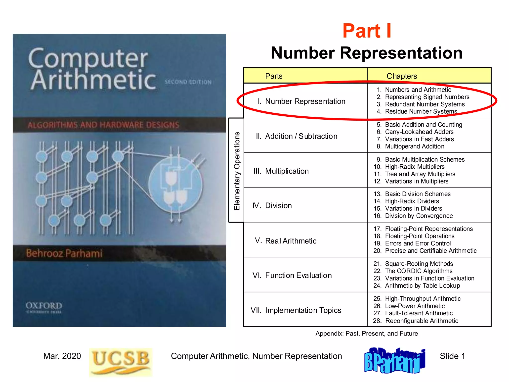
This document discusses number representation in computer arithmetic. It begins with an overview of topics related to number representation that will be covered, including fixed-radix positional number systems, signed numbers, redundant and residue number systems. It then provides examples of different number representation formats using 4 bits, such as unsigned integers, signed integers, signed fractions, and floating point. Radix conversion between different number bases is also discussed. The document provides background information on key concepts in number representation to set the framework for further chapters on arithmetic operations and number systems.

![Mar. 2020 Computer Arithmetic, Number Representation Slide 10
Using a calculator with √, x2, and xy functions, compute:
u = √√ … √ 2 = 1.000 677 131 “1024th root of 2”
v = 21/1024 = 1.000 677 131
Save u and v; If you can’t save, recompute values when needed
x = (((u2)2)...)2 = 1.999 999 963
x' = u1024 = 1.999 999 973
y = (((v2)2)...)2 = 1.999 999 983
y' = v1024 = 1.999 999 994
Perhaps v and u are not really the same value
w = v – u = 1 10–11 Nonzero due to hidden digits
(u – 1) 1000 = 0.677 130 680 [Hidden ... (0) 68]
(v – 1) 1000 = 0.677 130 690 [Hidden ... (0) 69]
1.2 A Motivating Example](https://image.slidesharecdn.com/f31-book-arith-pres-pt1-221120134844-1cb33af0/75/f31-book-arith-pres-pt1-ppt-10-2048.jpg)


![Mar. 2020 Computer Arithmetic, Number Representation Slide 14
Encoding Numbers in 4 Bits
Fig. 1.2 Some of the possible ways of assigning 16 distinct codes to
represent numbers. Small triangles denote the radix point locations.
0 2 4 6 8 10 12 14 16
-2
-4
-6
-8
-10
-12
-14
-16
Unsigned integers
Signed-magnitude
3 + 1 fixed-point, xxx.x
Signed fraction, .xxx
2’s-compl. fraction, x.xxx
2 + 2 floating-point, s 2
e in [-2, 1], s in [0, 3]
2 + 2 logarithmic (log = xx.xx)
Number
format
log x
s
e
e](https://image.slidesharecdn.com/f31-book-arith-pres-pt1-221120134844-1cb33af0/75/f31-book-arith-pres-pt1-ppt-14-2048.jpg)
![Mar. 2020 Computer Arithmetic, Number Representation Slide 15
1.4 Fixed-Radix Positional Number Systems
( xk–1xk–2 . . . x1x0 . x–1x–2 . . . x–l )r = xi ri
One can generalize to:
Arbitrary radix (not necessarily integer, positive, constant)
Arbitrary digit set, usually {–a, –a+1, . . . , b–1, b} = [–a, b]
Example 1.1. Balanced ternary number system:
Radix r = 3, digit set = [–1, 1]
Example 1.2. Negative-radix number systems:
Radix –r, r 2, digit set = [0, r – 1]
The special case with radix –2 and digit set [0, 1]
is known as the negabinary number system
-
-
1
k
l
i](https://image.slidesharecdn.com/f31-book-arith-pres-pt1-221120134844-1cb33af0/75/f31-book-arith-pres-pt1-ppt-15-2048.jpg)
![Mar. 2020 Computer Arithmetic, Number Representation Slide 16
More Examples of Number Systems
Example 1.3. Digit set [–4, 5] for r = 10:
(3 –1 5)ten represents 295 = 300 – 10 + 5
Example 1.4. Digit set [–7, 7] for r = 10:
(3 –1 5)ten = (3 0 –5)ten = (1 –7 0 –5)ten
Example 1.7. Quater-imaginary number system:
radix r = 2j, digit set [0, 3]](https://image.slidesharecdn.com/f31-book-arith-pres-pt1-221120134844-1cb33af0/75/f31-book-arith-pres-pt1-ppt-16-2048.jpg)


![Mar. 2020 Computer Arithmetic, Number Representation Slide 30
Arithmetic with Complement Representations
–––––––––––––––––––––––––––––––––––––––––––––––––––––––––––
Desired Computation to be Correct result Overflow
operation performed mod M with no overflow condition
–––––––––––––––––––––––––––––––––––––––––––––––––––––––––––
(+x) + (+y) x + y x + y x + y > P
(+x) + (–y) x + (M – y) x – y if y x N/A
M – (y – x) if y > x
(–x) + (+y) (M – x) + y y – x if x y N/A
M – (x – y) if x > y
(–x) + (–y) (M – x) + (M – y) M – (x + y) x + y > N
–––––––––––––––––––––––––––––––––––––––––––––––––––––––––––
Table 2.1 Addition in a complement number system with
complementation constant M and range [–N, +P]](https://image.slidesharecdn.com/f31-book-arith-pres-pt1-221120134844-1cb33af0/75/f31-book-arith-pres-pt1-ppt-30-2048.jpg)
![Mar. 2020 Computer Arithmetic, Number Representation Slide 31
Example and Two Special Cases
Example -- complement system for fixed-point numbers:
Complementation constant M = 12.000
Fixed-point number range [–6.000, +5.999]
Represent –3.258 as 12.000 – 3.258 = 8.742
Auxiliary operations for complement representations
complementation or change of sign (computing M – x)
computations of residues mod M
Thus, M must be selected to simplify these operations
Two choices allow just this for fixed-point radix-r arithmetic
with k whole digits and l fractional digits
Radix complement M = rk
Digit complement M = rk – ulp (aka diminished radix compl)
ulp (unit in least position) stands for r-l
Allows us to forget about l, even for nonintegers](https://image.slidesharecdn.com/f31-book-arith-pres-pt1-221120134844-1cb33af0/75/f31-book-arith-pres-pt1-ppt-31-2048.jpg)
![Mar. 2020 Computer Arithmetic, Number Representation Slide 32
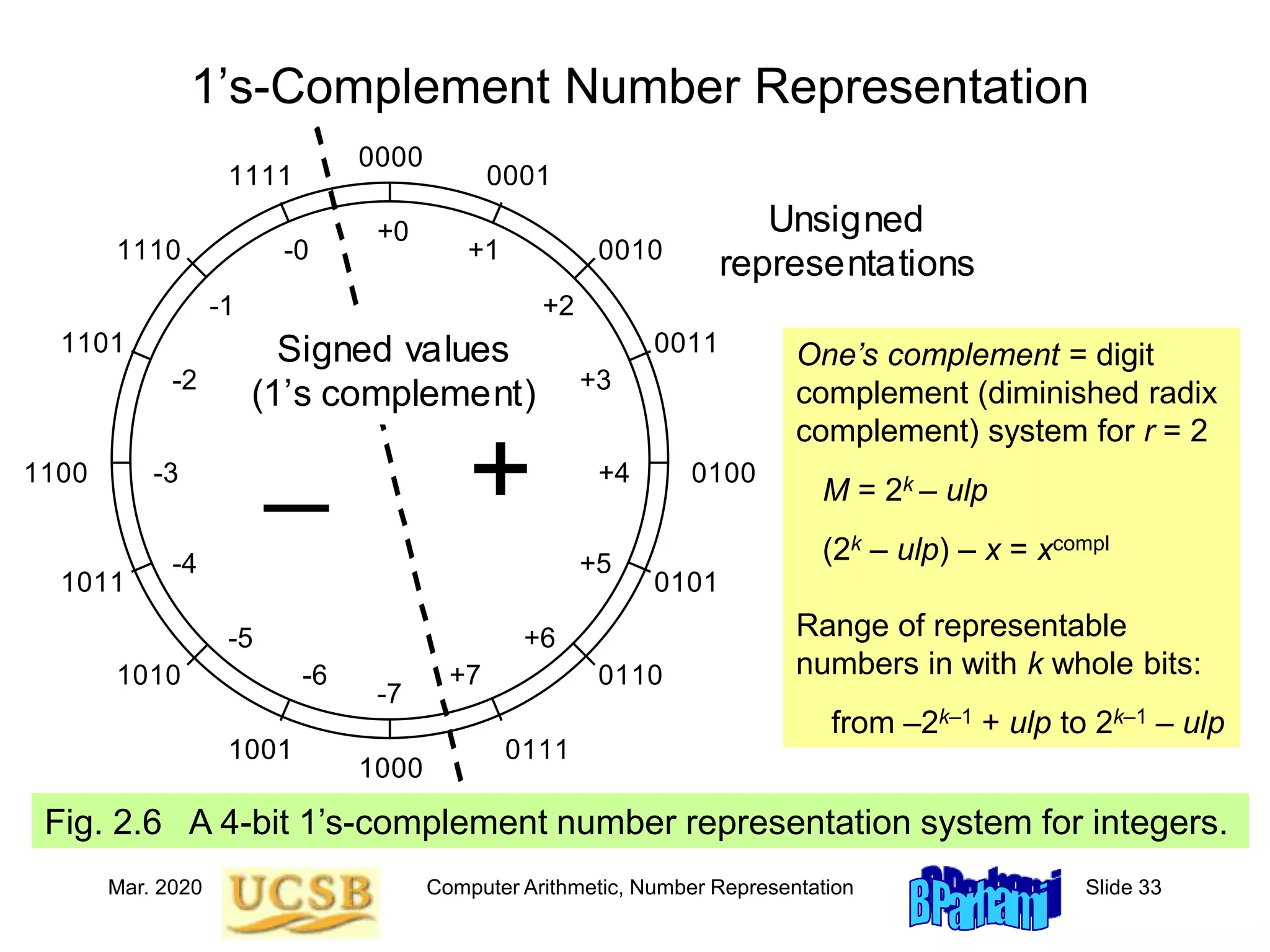
2.4 2’s- and 1’s-Complement Numbers
Fig. 2.5 A 4-bit 2’s-complement number representation system for integers.
0000
0001
1111
0010
1110
0011
1101
0100
1100
1000
0101
1011
0110
1010
0111
1001
+0
+1
+3
+4
+5
+6
+7
-1
-5
-3
-4
-8
-7
-6
+
_
Unsigned
representations
Signed values
(2’s complement)
+2
-2
Two’s complement = radix
complement system for r = 2
M = 2k
2k – x = [(2k – ulp) – x] + ulp
= xcompl + ulp
Range of representable
numbers in with k whole bits:
from –2k–1 to 2k–1 – ulp](https://image.slidesharecdn.com/f31-book-arith-pres-pt1-221120134844-1cb33af0/75/f31-book-arith-pres-pt1-ppt-32-2048.jpg)


![Mar. 2020 Computer Arithmetic, Number Representation Slide 40
Associating a Sign with Each Digit
Fig. 2.10 Converting a standard radix-4 integer to a radix-4
integer with the nonstandard digit set [–1, 2].
3 1 2 0 2 3 Original digits in [0, 3]
–1 1 2 0 2 –1
1 0 0 0 0 1
Rewritten digits in [–1, 2]
Transfer digits in [0, 1]
1 –1 1 2 0 3 –1
1 –1 1 2 0 –1 –1
0 0 0 0 1 0
1 –1 1 2 1 –1 –1
Sum digits in [–1, 3]
Rewritten digits in [–1, 2]
Transfer digits in [0, 1]
Sum digits in [–1, 3]
Signed-digit representation: Digit set [-a, b] instead of [0, r – 1]
Example: Radix-4 representation with digit set [-1, 2] rather than [0, 3]](https://image.slidesharecdn.com/f31-book-arith-pres-pt1-221120134844-1cb33af0/75/f31-book-arith-pres-pt1-ppt-40-2048.jpg)
![Mar. 2020 Computer Arithmetic, Number Representation Slide 41
Redundant Signed-Digit Representations
Fig. 2.11 Converting a standard radix-4 integer to a radix-4
integer with the nonstandard digit set [–2, 2].
Signed-digit representation: Digit set [-a, b], with r = a + b + 1 – r > 0
Example: Radix-4 representation with digit set [-2, 2]
3 1 2 0 2 3 Original digits in [0, 3]
–1 1 –2 0 –2 1
1 0 1 0 1 1
Interim digits in [–2, 1]
Transfer digits in [0, 1]
1 –1 2 –2 1 –1 –1 Sum digits in [–2, 2]
Here, the transfer does not propagate, so conversion is “carry-free”](https://image.slidesharecdn.com/f31-book-arith-pres-pt1-221120134844-1cb33af0/75/f31-book-arith-pres-pt1-ppt-41-2048.jpg)


![Mar. 2020 Computer Arithmetic, Number Representation Slide 46
3.1 Coping with the Carry Problem
Ways of dealing with the carry propagation problem:
1. Limit propagation to within a small number of bits (Chapters 3-4)
2. Detect end of propagation; don’t wait for worst case (Chapter 5)
3. Speed up propagation via lookahead etc. (Chapters 6-7)
4. Ideal: Eliminate carry propagation altogether! (Chapter 3)
5 7 8 2 4 9
6 2 9 3 8 9 Operand digits in [0, 9]
––––––––––––––––––––––––––––––––––
11 9 17 5 12 18 Position sums in [0, 18]
But how can we extend this beyond a single addition?
+](https://image.slidesharecdn.com/f31-book-arith-pres-pt1-221120134844-1cb33af0/75/f31-book-arith-pres-pt1-ppt-46-2048.jpg)
![Mar. 2020 Computer Arithmetic, Number Representation Slide 47
Addition of Redundant Numbers
Fig. 3.1 Adding radix-10 numbers with digit set [0, 18].
Position sum decomposition [0, 36] = 10 [0, 2] + [0, 16]
Absorption of transfer digit [0, 16] + [0, 2] = [0, 18]
6 12 9 10 8 18
Operand digits in [0, 18]
17 21 26 20 20 36
7 11 16 0 10 16
Position sums in [0, 36]
Interim sums in [0, 16]
1 1 1 2 1 2
1 8 12 18 1 12 16
11 9 17 10 12 18
Transfer digits in [0, 2]
Sum digits in [0, 18]
+](https://image.slidesharecdn.com/f31-book-arith-pres-pt1-221120134844-1cb33af0/75/f31-book-arith-pres-pt1-ppt-47-2048.jpg)
![Mar. 2020 Computer Arithmetic, Number Representation Slide 49
Redundancy Index
Fig. 3.3 Adding radix-10 numbers with digit set [0, 11].
So, redundancy helps us achieve carry-free addition
But how much redundancy is actually needed? Is [0, 11] enough for r = 10?
18 12 16 21 12 16 Position sums in [0, 22]
8 2 6 1 2 6
1 1 1 2 1 1
Interim sums in [0, 9]
Transfer digits in [0, 2]
1 9 3 8 2 3 6
11 10 7 11 3 8
Sum digits in [0, 11]
+ 7 2 9 10 9 8
Operand digits in [0, 11]
Redundancy index r = a + b + 1 – r For example, 0 + 11 + 1 – 10 = 2
-a b](https://image.slidesharecdn.com/f31-book-arith-pres-pt1-221120134844-1cb33af0/75/f31-book-arith-pres-pt1-ppt-49-2048.jpg)

![Mar. 2020 Computer Arithmetic, Number Representation Slide 51
Binary Carry-Save or Stored-Carry Representation
Fig. 3.4 Addition of
four binary numbers,
with the sum obtained
in stored-carry form.
0 0 1 0 0 1 First binary number
0 1 1 1 1 0
0 1 2 1 1 1
Add second binary number
Position sums in [0, 2]
+ 0 1 1 1 0 1 Add third binary number
Position sums in [0, 3]
Interim sums in [0, 1]
Transfer digits in [0, 1]
Position sums in [0, 2]
Add fourth binary number
Position sums in [0, 3]
0 2 3 2 1 2
0 0 1 0 1 0
0 1 1 1 0 1
1 1 2 0 2 0
+
1 1 3 0 3 1
1 1 1 0 1 1
0 0 1 0 1 0
1 2 1 1 1 1
+ 0 0 1 0 1 1
Interim sums in [0, 1]
Transfer digits in [0, 1]
Sum digits in [0, 2]
Oldest example of
redundancy in
computer arithmetic
is the stored-carry
representation
(carry-save addition)](https://image.slidesharecdn.com/f31-book-arith-pres-pt1-221120134844-1cb33af0/75/f31-book-arith-pres-pt1-ppt-51-2048.jpg)
![Mar. 2020 Computer Arithmetic, Number Representation Slide 52
Hardware for Carry-Save Addition
Fig. 3.5 Using an array of
independent binary full adders
to perform carry-save addition.
Binary
Full
Adder
(Stage i)
cin
cout
Digit in [0, 2] Binary digit
Digit in [0, 2]
To
Stage
i+1
From
Stage
i – 1
x y
s
Two-bit encoding for binary
stored-carry digits used in
this implementation:
0 represented as 0 0
1 represented as 0 1
or as 1 0
2 represented as 1 1
Because in carry-save addition,
three binary numbers are
reduced to two binary numbers,
this process is sometimes
referred to as 3-2 compression](https://image.slidesharecdn.com/f31-book-arith-pres-pt1-221120134844-1cb33af0/75/f31-book-arith-pres-pt1-ppt-52-2048.jpg)
![Mar. 2020 Computer Arithmetic, Number Representation Slide 53
Carry-Save Addition in Dot Notation
Two
carry-save
inputs
Carry-save
input
Binary input
Carry-save
output
This bit
being 1
represents
overflow
(ignore it)
0
0
0
a. Carry-save addition. b. Adding two carry-save numbers.
Carry-save
addition
Carry-save
addition
We sometimes find it convenient to use an extended dot notation,
with heavy dots (●) for posibits and hollow dots (○) for negabits
Eight-bit, 2’s-complement number ○ ● ● ● ● ● ● ●
Negative-radix number ○ ● ○ ● ○ ● ○ ●
BSD number with n, p encoding ○ ○ ○ ○ ○ ○ ○ ○
of the digit set [-1, 1] ● ● ● ● ● ● ● ●
Fig. 9.3 From text on computer architecture (Parhami, Oxford/2005)
3-to-2
reduction
4-to-2
reduction](https://image.slidesharecdn.com/f31-book-arith-pres-pt1-221120134844-1cb33af0/75/f31-book-arith-pres-pt1-ppt-53-2048.jpg)

![Mar. 2020 Computer Arithmetic, Number Representation Slide 55
3.3 Digit Sets and Digit-Set Conversions
Example 3.1: Convert from digit set [0, 18] to [0, 9] in radix 10
11 9 17 10 12 18 18 = 10 (carry 1) + 8
11 9 17 10 13 8 13 = 10 (carry 1) + 3
11 9 17 11 3 8 11 = 10 (carry 1) + 1
11 9 18 1 3 8 18 = 10 (carry 1) + 8
11 10 8 1 3 8 10 = 10 (carry 1) + 0
12 0 8 1 3 8 12 = 10 (carry 1) + 2
1 2 0 8 1 3 8 Answer;
all digits in [0, 9]
Note: Conversion from redundant to nonredundant representation
always involves carry propagation
Thus, the process is sequential and slow](https://image.slidesharecdn.com/f31-book-arith-pres-pt1-221120134844-1cb33af0/75/f31-book-arith-pres-pt1-ppt-55-2048.jpg)
![Mar. 2020 Computer Arithmetic, Number Representation Slide 56
Conversion from Carry-Save to Binary
Example 3.2: Convert from digit set [0, 2] to [0, 1] in radix 2
1 1 2 0 2 0 2 = 2 (carry 1) + 0
1 1 2 1 0 0 2 = 2 (carry 1) + 0
1 2 0 1 0 0 2 = 2 (carry 1) + 0
2 0 0 1 0 0 2 = 2 (carry 1) + 0
1 0 0 0 1 0 0 Answer;
all digits in [0, 1]
Another way: Decompose the carry-save number
into two numbers and add them:
1 1 1 0 1 0 1st number: sum bits
+ 0 0 1 0 1 0 2nd number: carry bits
––––––––––––––––––––––––––––––––––––––––
1 0 0 0 1 0 0 Sum](https://image.slidesharecdn.com/f31-book-arith-pres-pt1-221120134844-1cb33af0/75/f31-book-arith-pres-pt1-ppt-56-2048.jpg)
![Mar. 2020 Computer Arithmetic, Number Representation Slide 57
Conversion Between Redundant Digit Sets
Example 3.3: Convert from digit set [0, 18] to [-6, 5] in radix 10 (same as
Example 3.1, but with the target digit set signed and redundant)
11 9 17 10 12 18 18 = 20 (carry 2) – 2
11 9 17 10 14 -2 14 = 10 (carry 1) + 4
11 9 17 11 4 -2 11 = 10 (carry 1) + 1
11 9 18 1 4 -2 18 = 20 (carry 2) – 2
11 11 -2 1 4 -2 11 = 10 (carry 1) + 1
12 1 -2 1 4 -2 12 = 10 (carry 1) + 2
1 2 1 -2 1 4 -2 Answer;
all digits in [-6, 5]
On line 2, we could have written 14 = 20 (carry 2) – 6; this would have
led to a different, but equivalent, representation
In general, several representations may exist for a redundant digit set](https://image.slidesharecdn.com/f31-book-arith-pres-pt1-221120134844-1cb33af0/75/f31-book-arith-pres-pt1-ppt-57-2048.jpg)
![Mar. 2020 Computer Arithmetic, Number Representation Slide 58
Carry-Free Conversion to a Redundant Digit Set
Example 3.4: Convert from digit set [0, 2] to [-1, 1] in radix 2 (same as
Example 3.2, but with the target digit set signed and redundant)
Carry-free conversion:
1 1 2 0 2 0 Carry-save number
–1 –1 0 0 0 0 Interim digits in [–1, 0]
1 1 1 0 1 0 Transfer digits in [0, 1]
––––––––––––––––––––––––––––––––––––––––
1 0 0 0 1 0 0 Answer;
all digits in [–1, 1]
We rewrite 2 as 2 (carry 1) + 0, and 1 as 2 (carry 1) – 1
A carry of 1 is always absorbed by the interim digit that is in {-1, 0}](https://image.slidesharecdn.com/f31-book-arith-pres-pt1-221120134844-1cb33af0/75/f31-book-arith-pres-pt1-ppt-58-2048.jpg)
![Mar. 2020 Computer Arithmetic, Number Representation Slide 59
3.4 Generalized Signed-Digit Numbers
Fig. 3.6
A taxonomy of
redundant and
non-redundant
positional
number
systems.
Radix-r Positional
r r
Non-redundant
a a
Conventional Non-redundant
signed-digit
Generalized
signed-digit (GSD)
r r
Minimal
GSD
Non-minimal
GSD
ab
(even r)
ab
Symmetric
minimal GSD
r = 2
BSD or
BSB
Asymmetric
minimal GSD
a a
(r ° 2)
Stored-
carry (SC)
Non-binary
SB
Symmetric non-
minimal GSD
ab ab
Asymmetric non-
minimal GSD
a r
Ordinary
signed-digit
Minimally
redundant OSD
Maximally
redundant OSD BSCB
SCB
r = 2
a
b r
a
Unsigned-digit
redundant (UDR)
r = 2
BSC
a r – 1
a
r/2 + 1
Radix r
Digit set [–a, b]
Requirement
a + b + 1 r
Redundancy index
r = a + b + 1 – r](https://image.slidesharecdn.com/f31-book-arith-pres-pt1-221120134844-1cb33af0/75/f31-book-arith-pres-pt1-ppt-59-2048.jpg)
![Mar. 2020 Computer Arithmetic, Number Representation Slide 60
Encodings for Signed Digits
Fig. 3.7 Four encodings for the BSD digit set [–1, 1].
xi
s, v
2’s-compl
n, p
n, z, p
Two of the
encodings
above
can be shown
in extended
dot notation
Fig. 3.8 Extended dot notation and its use in visualizing
some BSD encodings.
Posibit {0, 1}
Negabit {–1, 0}
Doublebit {0, 2}
Negadoublebit {–2, 0}
Unibit {–1, 1}
(a) Extended dot notation
(n, p) encoding
2’s-compl. encoding
2’s-compl. encoding
(b) Encodings for a BSD number
BSD representation of +6
Sign and value encoding
2-bit 2’s-complement
Negative & positive flags
1-out-of-3 encoding
0
00
00
00
010
–1
11
11
10
100
0
00
00
00
010
–1
11
11
10
100
1
01
01
01
001](https://image.slidesharecdn.com/f31-book-arith-pres-pt1-221120134844-1cb33af0/75/f31-book-arith-pres-pt1-ppt-60-2048.jpg)
![Mar. 2020 Computer Arithmetic, Number Representation Slide 61
Hybrid Signed-Digit Numbers
i
i
i
i
i
BSD B B BSD B B Type
1 0 1 –1 0 1
+ 0 1 1 –1 1
x
y
1 1 2 –2 1 1
–1 0
1 –1 0
1 –1 1 1 0 1 1
p
w
t
s
BSD B B
–1 0 1
–1 1 1
–1 1 1
0 1 0
–1
0
i+1
Fig. 3.9 Example of addition for hybrid signed-digit numbers.
Radix-8
GSD
with
digit set
[-4,7]
The hybrid-redundant representation above in extended dot notation:
n, p -encoded ○ ● ● ○ ● ● ○ ● ● Nonredundant
binary signed digit ● ● ● binary positions](https://image.slidesharecdn.com/f31-book-arith-pres-pt1-221120134844-1cb33af0/75/f31-book-arith-pres-pt1-ppt-61-2048.jpg)
![Mar. 2020 Computer Arithmetic, Number Representation Slide 62
Hybrid Redundancy in Extended Dot Notation
Fig. 3.10 Two hybrid-redundant representations in extended
dot notation.
Radix-8 digit set [–4, 7]
Radix-8 digit set [–4, 4]](https://image.slidesharecdn.com/f31-book-arith-pres-pt1-221120134844-1cb33af0/75/f31-book-arith-pres-pt1-ppt-62-2048.jpg)
![Mar. 2020 Computer Arithmetic, Number Representation Slide 63
3.5 Carry-Free Addition Algorithms
Carry-free addition of GSD numbers
Compute the position sums pi = xi + yi
Divide pi into a transfer ti+1 and interim sum wi = pi – rti+1
Add incoming transfers to get the sum digits si = wi + ti
xi–1,yi–1
,
xi
xi+1,yi+1 yi
si+1 si–1
si
ti
wi
If the transfer digits ti are in [–l, m], we must have:
–a + l pi – rti+1 b – m
interim sum
Smallest interim sum Largest interim sum
if a transfer of –l if a transfer of m
is to be absorbable is to be absorbable
These
constraints
lead to:
l a / (r – 1)
m b / (r – 1)](https://image.slidesharecdn.com/f31-book-arith-pres-pt1-221120134844-1cb33af0/75/f31-book-arith-pres-pt1-ppt-63-2048.jpg)
![Mar. 2020 Computer Arithmetic, Number Representation Slide 64
Is Carry-Free Addition Always Applicable?
No: It requires one of the following two conditions
a. r > 2, r 3
b. r > 2, r = 2, a 1, b 1 e.g., not [-1, 10] in radix 10
In other words, it is inapplicable for
r = 2 Perhaps most useful case
r = 1 e.g., carry-save
r = 2 with a = 1 or b = 1 e.g., carry/borrow-save
BSD fails on at least two criteria!
Fortunately, in the latter cases, a limited-carry
addition algorithm is always applicable](https://image.slidesharecdn.com/f31-book-arith-pres-pt1-221120134844-1cb33af0/75/f31-book-arith-pres-pt1-ppt-64-2048.jpg)

![Mar. 2020 Computer Arithmetic, Number Representation Slide 66
Limited-Carry BSD Addition
Fig. 3.13 Limited-carry addition of radix-2 numbers with digit set [–1, 1]
using carry estimates. A position sum –1 is kept intact when the incoming
transfer is in [0, 1], whereas it is rewritten as 1 with a carry of –1 for
incoming transfer in [–1, 0]. This guarantees that ti wi and thus –1 si 1.
1 –1 0 –1 0 x in [–1, 1]
+ 0 –1 –1 0 1
1 –2 –1 –1 1
1 0 1 –1 –1
–1 –1 0 1
0 –1 1 0 –1
i
i+1
y in [–1, 1]
i
p in [–2, 2]
i
w in [–1, 1]
i
s in [–1, 1]
i
t in [–1, 1]
low low low high high
high
0
0
e in {low: [–1, 0], high: [0, 1]}
i](https://image.slidesharecdn.com/f31-book-arith-pres-pt1-221120134844-1cb33af0/75/f31-book-arith-pres-pt1-ppt-66-2048.jpg)


![Mar. 2020 Computer Arithmetic, Number Representation Slide 72
RNS Dynamic Range
Product M of the k pairwise relatively prime moduli is the dynamic range
M = mk–1 . . . m1 m0
For RNS(8 | 7 | 5 | 3), M = 8753 = 840
Negative numbers: Complement relative to M
–xmi
= M – xmi
21 = (5 | 0 | 1 | 0)RNS
–21 = (8 – 5 | 0 | 5 – 1 | 0)RNS = (3 | 0 | 4 | 0)RNS
Here are some example numbers in our default RNS(8 | 7 | 5 | 3):
(0 | 0 | 0 | 0)RNS Represents 0 or 840 or . . .
(1 | 1 | 1 | 1)RNS Represents 1 or 841 or . . .
(2 | 2 | 2 | 2)RNS Represents 2 or 842 or . . .
(0 | 1 | 3 | 2)RNS Represents 8 or 848 or . . .
(5 | 0 | 1 | 0)RNS Represents 21 or 861 or . . .
(0 | 1 | 4 | 1)RNS Represents 64 or 904 or . . .
(2 | 0 | 0 | 2)RNS Represents –70 or 770 or . . .
(7 | 6 | 4 | 2)RNS Represents –1 or 839 or . . .
We can take the
range of RNS(8|7|5|3)
to be [-420, 419] or
any other set of 840
consecutive integers](https://image.slidesharecdn.com/f31-book-arith-pres-pt1-221120134844-1cb33af0/75/f31-book-arith-pres-pt1-ppt-72-2048.jpg)


![Mar. 2020 Computer Arithmetic, Number Representation Slide 75
4.2 Choosing the RNS Moduli
Target range for our RNS: Decimal values [0, 100 000]
Strategy 1: To minimize the largest modulus, and thus ensure
high-speed arithmetic, pick prime numbers in sequence
Pick m0 = 2, m1 = 3, m2 = 5, etc. After adding m5 = 13:
RNS(13 | 11 | 7 | 5 | 3 | 2) M = 30 030 Inadequate
RNS(17 | 13 | 11 | 7 | 5 | 3 | 2) M = 510 510 Too large
RNS(17 | 13 | 11 | 7 | 3 | 2) M = 102 102 Just right!
5 + 4 + 4 + 3 + 2 + 1 = 19 bits
Fine tuning: Combine pairs of moduli 2 & 13 (26) and 3 & 7 (21)
RNS(26 | 21 | 17 | 11) M = 102 102](https://image.slidesharecdn.com/f31-book-arith-pres-pt1-221120134844-1cb33af0/75/f31-book-arith-pres-pt1-ppt-75-2048.jpg)
![Mar. 2020 Computer Arithmetic, Number Representation Slide 76
An Improved Strategy
Target range for our RNS: Decimal values [0, 100 000]
Strategy 2: Improve strategy 1 by including powers of smaller
primes before proceeding to the next larger prime
RNS(22 | 3) M = 12
RNS(32 | 23 | 7 | 5) M = 2520
RNS(11 | 32 | 23 | 7 | 5) M = 27 720
RNS(13 | 11 | 32 | 23 | 7 | 5) M = 360 360
(remove one 3, combine 3 & 5)
RNS(15 | 13 | 11 | 23 | 7) M = 120 120
4 + 4 + 4 + 3 + 3 = 18 bits
Fine tuning: Maximize the size of the even modulus within the 4-bit limit
RNS(24 | 13 | 11 | 32 | 7 | 5) M = 720 720 Too large
We can now remove 5 or 7; not an improvement in this example](https://image.slidesharecdn.com/f31-book-arith-pres-pt1-221120134844-1cb33af0/75/f31-book-arith-pres-pt1-ppt-76-2048.jpg)
![Mar. 2020 Computer Arithmetic, Number Representation Slide 77
Low-Cost RNS Moduli
Target range for our RNS: Decimal values [0, 100 000]
Strategy 3: To simplify the modular reduction (mod mi) operations,
choose only moduli of the forms 2a or 2a – 1, aka “low-cost moduli”
RNS(2ak–1 | 2ak–2 – 1 | . . . | 2a1 – 1 | 2a0 – 1)
We can have only one even modulus
2ai – 1 and 2aj – 1 are relatively prime iff ai and aj are relatively prime
RNS(23 | 23–1 | 22–1) basis: 3, 2 M = 168
RNS(24 | 24–1 | 23–1) basis: 4, 3 M = 1680
RNS(25 | 25–1 | 23–1 | 22–1) basis: 5, 3, 2 M = 20 832
RNS(25 | 25–1 | 24–1 | 23–1) basis: 5, 4, 3 M = 104 160
Comparison
RNS(15 | 13 | 11 | 23 | 7) 18 bits M = 120 120
RNS(25 | 25–1 | 24–1 | 23–1) 17 bits M = 104 160](https://image.slidesharecdn.com/f31-book-arith-pres-pt1-221120134844-1cb33af0/75/f31-book-arith-pres-pt1-ppt-77-2048.jpg)
![Mar. 2020 Computer Arithmetic, Number Representation Slide 78
Low- and Moderate-Cost RNS Moduli
Target range for our RNS: Decimal values [0, 100 000]
Strategy 4: To simplify the modular reduction (mod mi) operations,
choose moduli of the forms 2a, 2a – 1, or 2a + 1
RNS(2ak–1 | 2ak–2 1 | . . . | 2a1 1 | 2a0 1)
We can have only one even modulus
2ai – 1 and 2aj + 1 are relatively prime
RNS(25 | 24–1 | 24+1 | 23–1) M = 57 120
RNS(25 | 24+1 | 23+1 | 23–1 | 22–1) M = 102 816
Neither 5 nor 3 is acceptable
The modulus 2a + 1 is not as convenient as 2a – 1
(needs an extra bit for residue, and modular operations are not as simple)
Diminished-1 representation of values in [0, 2a] is a way to simplify things
Represent 0 by a special flag bit and nonzero values by coding one less](https://image.slidesharecdn.com/f31-book-arith-pres-pt1-221120134844-1cb33af0/75/f31-book-arith-pres-pt1-ppt-78-2048.jpg)


![Mar. 2020 Computer Arithmetic, Number Representation Slide 82
Conversion from RNS to Mixed-Radix Form
MRS(mk–1 | . . . | m2 | m1 | m0) is a k-digit positional system with weights
mk–2...m2m1m0 . . . m2m1m0 m1m0 m0 1
and digit sets
[0, mk–1–1] . . . [0,m3–1] [0,m2–1] [0,m1–1] [0,m0–1]
Example: (0 | 3 | 1 | 0)MRS(8|7|5|3) = 0105 + 315 + 13 + 01 = 48
RNS-to-MRS conversion problem:
y = (xk–1 | . . . | x2 | x1 | x0)RNS = (zk–1 | . . . | z2 | z1 | z0)MRS
MRS representation allows magnitude comparison and sign detection
Example: 48 versus 45
(0 | 6 | 3 | 0)RNS vs (5 | 3 | 0 | 0)RNS
(000 | 110 | 011 | 00)RNS vs (101 | 011 | 000 | 00)RNS
Equivalent mixed-radix representations
(0 | 3 | 1 | 0)MRS vs (0 | 3 | 0 | 0)MRS
(000 | 011 | 001 | 00)MRS vs (000 | 011 | 000 | 00)MRS](https://image.slidesharecdn.com/f31-book-arith-pres-pt1-221120134844-1cb33af0/75/f31-book-arith-pres-pt1-ppt-82-2048.jpg)

![Mar. 2020 Computer Arithmetic, Number Representation Slide 85
4.4 Difficult RNS Arithmetic Operations
Sign test and magnitude comparison are difficult
Example: Of the following RNS(8 | 7 | 5 | 3) numbers:
Which, if any, are negative?
Which is the largest?
Which is the smallest?
Assume a range of [–420, 419]
a = (0 | 1 | 3 | 2)RNS
b = (0 | 1 | 4 | 1)RNS
c = (0 | 6 | 2 | 1)RNS
d = (2 | 0 | 0 | 2)RNS
e = (5 | 0 | 1 | 0)RNS
f = (7 | 6 | 4 | 2)RNS
Answers:
d < c < f < a < e < b
–70 < –8 < –1 < 8 < 21 < 64](https://image.slidesharecdn.com/f31-book-arith-pres-pt1-221120134844-1cb33af0/75/f31-book-arith-pres-pt1-ppt-85-2048.jpg)
![Mar. 2020 Computer Arithmetic, Number Representation Slide 88
4.5 Redundant RNS Representations
Fig. 4.3 Adding a 4-bit ordinary
mod-13 residue x to a 4-bit
pseudoresidue y, producing a
4-bit mod-13 pseudoresidue z.
Adder
Adder
x y
z
cout
0 0
Drop
Pseudoresidue x Residue y
Pseudoresidue z
Drop
Adder
Adder
Fig. 4.4 A modulo-m
multiply-add cell that accumulates
the sum into a double-length
redundant pseudoresidue.
[0, 15] [0, 12]
[0, 15]
[0, 11]
if cout = 1
[0, 15]](https://image.slidesharecdn.com/f31-book-arith-pres-pt1-221120134844-1cb33af0/75/f31-book-arith-pres-pt1-ppt-88-2048.jpg)
![Mar. 2020 Computer Arithmetic, Number Representation Slide 89
4.6 Limits of Fast Arithmetic in RNS
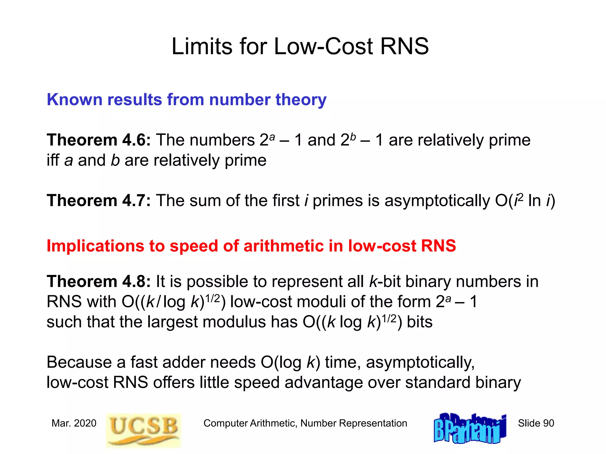
Known results from number theory
Implications to speed of arithmetic in RNS
Theorem 4.5: It is possible to represent all k-bit binary numbers
in RNS with O(k / log k) moduli such that the largest modulus
has O(log k) bits
That is, with fast log-time adders, addition needs O(log log k) time
Theorem 4.2: The ith prime pi is asymptotically i ln i
Theorem 4.3: The number of primes in [1, n] is asymptotically n/ln n
Theorem 4.4: The product of all primes in [1, n] is asymptotically en](https://image.slidesharecdn.com/f31-book-arith-pres-pt1-221120134844-1cb33af0/75/f31-book-arith-pres-pt1-ppt-89-2048.jpg)