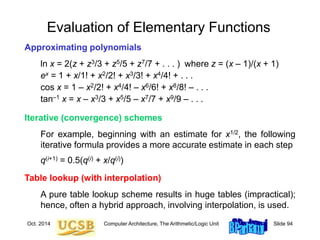
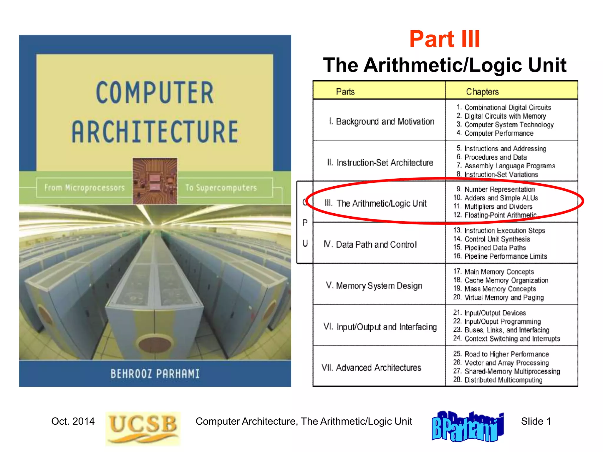
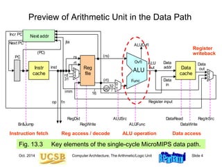
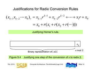
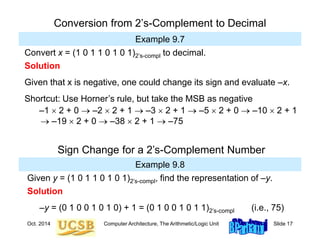
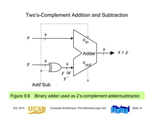
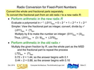
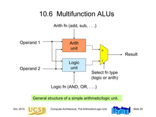
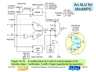
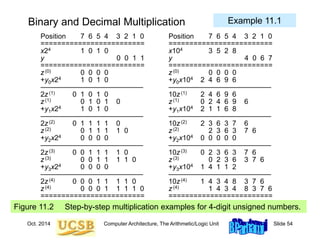
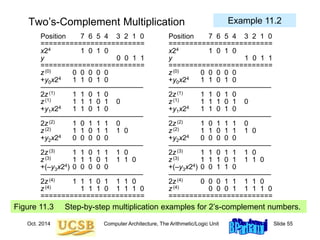
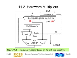
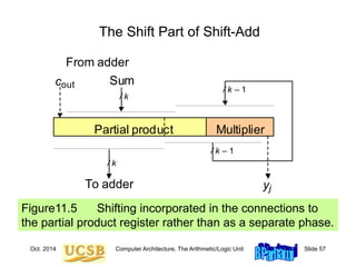
The presentation discusses the arithmetic/logic unit (ALU) of a computer. It provides an overview of topics related to computer arithmetic including number representation methods, addition and multiplication algorithms, and floating-point representation and arithmetic. The ALU performs arithmetic and logical operations and is a key component in the datapath of a processor. Number representation, such as binary, hexadecimal, and floating-point, affects the ease of performing arithmetic operations in hardware.


![Oct. 2014 Computer Architecture, The Arithmetic/Logic Unit Slide 7
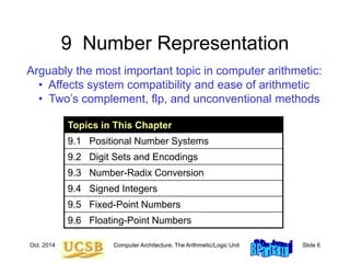
9.1 Positional Number Systems
Representations of natural numbers {0, 1, 2, 3, …}
||||| ||||| ||||| ||||| ||||| || sticks or unary code
27 radix-10 or decimal code
11011 radix-2 or binary code
XXVII Roman numerals
Fixed-radix positional representation with k digits
Value of a number: x = (xk–1xk–2 . . . x1x0)r = S xi r i
For example:
27 = (11011)two = (124) + (123) + (022) + (121) + (120)
Number of digits for [0, P]: k = logr (P + 1) = logr P + 1
k–1
i=0](https://image.slidesharecdn.com/f37-book-intarch-pres-pt3-230913163318-64bba6b0/85/CA-ppt-7-320.jpg)
![Oct. 2014 Computer Architecture, The Arithmetic/Logic Unit Slide 8
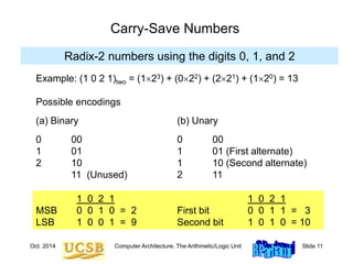
Unsigned Binary Integers
Figure 9.1 Schematic representation of 4-bit code for
integers in [0, 15].
0000
0001
1111
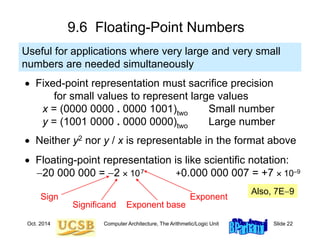
0010
1110
0011
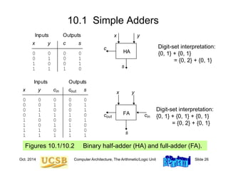
1101
0100
1100
1000
0101
1011
0110
1010
0111
1001
0
1
2
3
4
5
6
7
15
11
14
13
12
8
9
10
Inside: Natural number
Outside: 4-bit encoding
0
1
2
3
15
4
5
6
7
8
9
Turn x notches
counterclockwise
to add x
Turn y notches
clockwise
to subtract y
11
14
13
12
10](https://image.slidesharecdn.com/f37-book-intarch-pres-pt3-230913163318-64bba6b0/85/CA-ppt-8-320.jpg)
![Oct. 2014 Computer Architecture, The Arithmetic/Logic Unit Slide 9
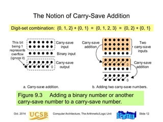
Representation Range and Overflow
Figure 9.2 Overflow regions in finite number representation systems.
For unsigned representations covered in this section, max – = 0.
max
Finite set of representable numbers
Overflow region
max
Overflow region
Numbers larger
than max
Numbers smaller
than max
Example 9.2, Part d
Discuss if overflow will occur when computing 317 – 316 in a number
system with k = 8 digits in radix r = 10.
Solution
The result 86 093 442 is representable in the number system which
has a range [0, 99 999 999]; however, if 317 is computed en route to
the final result, overflow will occur.](https://image.slidesharecdn.com/f37-book-intarch-pres-pt3-230913163318-64bba6b0/85/CA-ppt-9-320.jpg)
![Oct. 2014 Computer Architecture, The Arithmetic/Logic Unit Slide 10
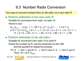
9.2 Digit Sets and Encodings
Conventional and unconventional digit sets
Decimal digits in [0, 9]; 4-bit BCD, 8-bit ASCII
Hexadecimal, or hex for short: digits 0-9 & a-f
Conventional ternary digit set in [0, 2]
Conventional digit set for radix r is [0, r – 1]
Symmetric ternary digit set in [–1, 1]
Conventional binary digit set in [0, 1]
Redundant digit set [0, 2], encoded in 2 bits
( 0 2 1 1 0 )two and ( 1 0 1 0 2 )two represent 22](https://image.slidesharecdn.com/f37-book-intarch-pres-pt3-230913163318-64bba6b0/85/CA-ppt-10-320.jpg)
![Oct. 2014 Computer Architecture, The Arithmetic/Logic Unit Slide 15
9.4 Signed Integers
We dealt with representing the natural numbers
Signed or directed whole numbers = integers
{ . . . , 3, 2, 1, 0, 1, 2, 3, . . . }
Signed-magnitude representation
+27 in 8-bit signed-magnitude binary code 0 0011011
–27 in 8-bit signed-magnitude binary code 1 0011011
–27 in 2-digit decimal code with BCD digits 1 0010 0111
Biased representation
Represent the interval of numbers [N, P] by the unsigned
interval [0, P + N]; i.e., by adding N to every number](https://image.slidesharecdn.com/f37-book-intarch-pres-pt3-230913163318-64bba6b0/85/CA-ppt-15-320.jpg)
![Oct. 2014 Computer Architecture, The Arithmetic/Logic Unit Slide 16
Two’s-Complement Representation
Figure 9.5 Schematic representation of 4-bit 2’s-complement
code for integers in [–8, +7].
0000
0001
1111
0010
1110
0011
1101
0100
1100
1000
0101
1011
0110
1010
0111
1001
+0
+1
+2
+3
+4
+5
+6
+7
–1
–5
–2
–3
–4
–8
–7
–6
+
_
0
1
2
3
–1
4
5
6
7
–8
–7
Turn x notches
counterclockwise
to add x
Turn 16 – y notches
counterclockwise to
add –y (subtract y)
–5
–2
–3
–4
–6
With k bits, numbers in the range [–2k–1, 2k–1 – 1] represented.
Negation is performed by inverting all bits and adding 1.](https://image.slidesharecdn.com/f37-book-intarch-pres-pt3-230913163318-64bba6b0/85/CA-ppt-16-320.jpg)
![Oct. 2014 Computer Architecture, The Arithmetic/Logic Unit Slide 19
9.5 Fixed-Point Numbers
Positional representation: k whole and l fractional digits
Value of a number: x = (xk–1xk–2 . . .x1x0 .x–1x–2 . . . x–l )r = S xi r i
For example:
2.375 = (10.011)two = (121) + (020) + (021) + (122) + (123)
Numbers in the range [0, rk – ulp] representable, where ulp = r –l
Fixed-point arithmetic same as integer arithmetic
(radix point implied, not explicit)
Two’s complement properties (including sign change) hold here as well:
(01.011)2’s-compl = (–021) + (120) + (02–1) + (12–2) + (12–3) = +1.375
(11.011)2’s-compl = (–121) + (120) + (02–1) + (12–2) + (12–3) = –0.625](https://image.slidesharecdn.com/f37-book-intarch-pres-pt3-230913163318-64bba6b0/85/CA-ppt-19-320.jpg)
![Oct. 2014 Computer Architecture, The Arithmetic/Logic Unit Slide 20
Fixed-Point 2’s-Complement Numbers
Figure 9.7 Schematic representation of 4-bit 2’s-complement
encoding for (1 + 3)-bit fixed-point numbers in the range [–1, +7/8].
0.000
0.001
1.111
0.010
1.110
0.011
1.101
0.100
1.100
1.000
0.101
1.011
0.110
1.010
0.111
1.001
+0
+.125
+.25
+.375
+.5
+.625
+.75
+.875
–.125
–.625
–.25
–.375
–.5
–1
–.875
–.75
+
_](https://image.slidesharecdn.com/f37-book-intarch-pres-pt3-230913163318-64bba6b0/85/CA-ppt-20-320.jpg)
![Oct. 2014 Computer Architecture, The Arithmetic/Logic Unit Slide 24
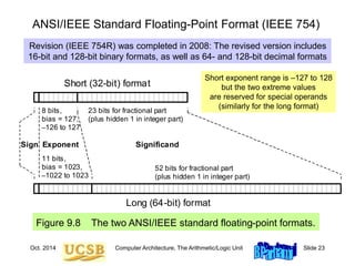
Short and Long IEEE 754 Formats: Features
Table 9.1 Some features of ANSI/IEEE standard floating-point formats
Feature Single/Short Double/Long
Word width in bits 32 64
Significand in bits 23 + 1 hidden 52 + 1 hidden
Significand range [1, 2 – 2–23] [1, 2 – 2–52]
Exponent bits 8 11
Exponent bias 127 1023
Zero (±0) e + bias = 0, f = 0 e + bias = 0, f = 0
Denormal e + bias = 0, f ≠ 0
represents ±0.f 2–126
e + bias = 0, f ≠ 0
represents ±0.f 2–1022
Infinity (∞) e + bias = 255, f = 0 e + bias = 2047, f = 0
Not-a-number (NaN) e + bias = 255, f ≠ 0 e + bias = 2047, f ≠ 0
Ordinary number e + bias [1, 254]
e [–126, 127]
represents 1.f 2e
e + bias [1, 2046]
e [–1022, 1023]
represents 1.f 2e
min 2–126 1.2 10–38 2–1022 2.2 10–308
max 2128 3.4 1038 21024 1.8 10308
Subnormal](https://image.slidesharecdn.com/f37-book-intarch-pres-pt3-230913163318-64bba6b0/85/CA-ppt-24-320.jpg)
![Oct. 2014 Computer Architecture, The Arithmetic/Logic Unit Slide 35
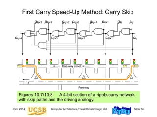
Mux-Based Skip Carry Logic
The carry-skip adder of Fig. 10.7 works fine if we begin with a
clean slate, where all signals are 0s; otherwise, it will run into
problems, which do not exist in this mux-based implementation
c
g p4j+1
4j+1 g p4j
4j
g p4j+2
4j+2
g p4j+3
4j+3
c4j
4j+4 c4j+3 c4j+2 c4j+1
0
1
p[4j, 4j+3]
c4j+4
c
g p4j+1
4j+1 g p4j
4j
g p4j+2
4j+2
g p4j+3
4j+3
c4j
4j+4 c4j+3 c4j+2 c4j+1
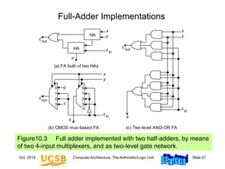
Fig. 10.7](https://image.slidesharecdn.com/f37-book-intarch-pres-pt3-230913163318-64bba6b0/85/CA-ppt-35-320.jpg)
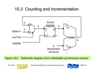
![Oct. 2014 Computer Architecture, The Arithmetic/Logic Unit Slide 38
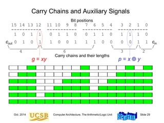
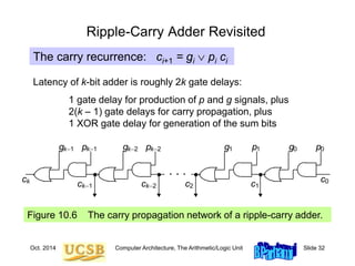
Carries can be computed directly without propagation
For example, by unrolling the equation for c3, we get:
c3 = g2 p2 c2 = g2 p2 g1 p2 p1 g0 p2 p1 p0 c0
We define “generate” and “propagate” signals for a block
extending from bit position a to bit position b as follows:
g[a,b] = gb pb gb–1 pb pb–1gb–2 . . . pb pb–1…pa+1 ga
p[a,b] = pb pb–1. . . pa+1 pa
Combining g and p signals for adjacent blocks:
g[h,j] = g[i+1,j] p[i+1,j] g[h,i]
p[h,j] = p[i+1,j] p[h,i]
10.4 Design of Fast Adders
h
i
i+1
j
[h, j] = [i + 1, j] ¢ [h, i]](https://image.slidesharecdn.com/f37-book-intarch-pres-pt3-230913163318-64bba6b0/85/CA-ppt-38-320.jpg)
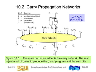
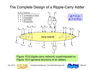
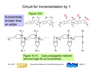
![Oct. 2014 Computer Architecture, The Arithmetic/Logic Unit Slide 39
Carries as Generate Signals for Blocks [ 0, i]
Figure 10.5
Carry network
. . . . . .
xi
yi
g p
s
i
i
i
ci
ci+1
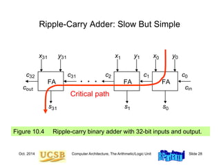
ck1
ck
ck2
c1
c0
g p1
1 g p0
0
g pk2
k2
g pi+1
i+1
g pk1
k1
c0
. . . . . .
0 0
0 1
1 0
1 1
annihilated or killed
propagated
generated
(impossible)
Carry is:
gi
pi
Assuming c0 = 0,
we have ci = g[0,i –1]](https://image.slidesharecdn.com/f37-book-intarch-pres-pt3-230913163318-64bba6b0/85/CA-ppt-39-320.jpg)
![Oct. 2014 Computer Architecture, The Arithmetic/Logic Unit Slide 40
Second Carry Speed-Up Method: Carry Lookahead
Figure 10.11 Brent-Kung lookahead carry network for an 8-digit adder,
along with details of one of the carry operator blocks.
¢ ¢ ¢ ¢
¢ ¢
¢ ¢
¢ ¢ ¢
[7, 7] [6, 6] [5, 5] [4, 4] [3, 3] [2, 2] [1, 1] [0, 0]
[0, 7] [0, 6] [0, 5] [0, 4] [0, 3] [0, 2] [0, 1] [0, 0]
[2, 3]
[4, 5]
[6, 7]
[4, 7]
[0, 3]
[0, 1]
g[0, 0]
g[0, 1]
g[1, 1]
p[0, 0]
p[0, 1]
p[1, 1]](https://image.slidesharecdn.com/f37-book-intarch-pres-pt3-230913163318-64bba6b0/85/CA-ppt-40-320.jpg)
![Oct. 2014 Computer Architecture, The Arithmetic/Logic Unit Slide 41
Recursive Structure of Brent-Kung Carry Network
Figure 10.12 Brent-Kung lookahead carry network for an 8-digit adder,
with only its top and bottom rows of carry-operators shown.
¢ ¢ ¢ ¢
¢ ¢ ¢
[7, 7] [6, 6] [5, 5] [4, 4] [3, 3] [2, 2] [1, 1] [0, 0]
[0, 7] [0, 6] [0, 5] [0, 4] [0, 3] [0, 2] [0, 1] [0, 0]
4-input Brent-Kung
carry network
¢ ¢ ¢ ¢
¢ ¢
¢ ¢
¢ ¢ ¢
[7, 7] [6, 6] [5, 5] [4, 4] [3, 3] [2, 2] [1, 1] [0, 0]
[0, 7] [0, 6] [0, 5] [0, 4] [0, 3] [0, 2] [0, 1] [0, 0]
[2, 3]
[4, 5]
[6, 7]
[4, 7]
[0, 3]
[0, 1]](https://image.slidesharecdn.com/f37-book-intarch-pres-pt3-230913163318-64bba6b0/85/CA-ppt-41-320.jpg)
![Oct. 2014 Computer Architecture, The Arithmetic/Logic Unit Slide 42
An Alternate Design: Kogge-Stone Network
Kogge-Stone lookahead carry network for an 8-digit adder.
¢ ¢ ¢ ¢
¢ ¢ ¢ ¢
¢ ¢
¢ ¢
¢ ¢
¢
¢ ¢
c1 = g[0,0]
c2 = g[0,1]
c3 = g[0,2]
c8 = g[0,7] c4 = g[0,3]
c5 = g[0,4]
c6 = g[0,5]
c7 = g[0,6]](https://image.slidesharecdn.com/f37-book-intarch-pres-pt3-230913163318-64bba6b0/85/CA-ppt-42-320.jpg)
![Oct. 2014 Computer Architecture, The Arithmetic/Logic Unit Slide 43
¢ ¢ ¢ ¢
¢ ¢
¢ ¢
¢ ¢ ¢
[7, 7] [6, 6] [5, 5] [4, 4] [3, 3] [2, 2] [1, 1] [0, 0]
[0, 7] [0, 6] [0, 5] [0, 4] [0, 3] [0, 2] [0, 1] [0, 0]
[2, 3]
[4, 5]
[6, 7]
[4, 7]
[0, 3]
[0, 1]
g[0, 0]
g[0, 1]
g[1, 1]
p[0, 0]
p[0, 1]
p[1, 1]
Brent-Kung vs. Kogge-Stone Carry Network
11 carry operators
4 levels
17 carry operators
3 levels](https://image.slidesharecdn.com/f37-book-intarch-pres-pt3-230913163318-64bba6b0/85/CA-ppt-43-320.jpg)
![Oct. 2014 Computer Architecture, The Arithmetic/Logic Unit Slide 44
Carry-Lookahead Logic with 4-Bit Block
Figure 10.13 Blocks needed in the design of carry-lookahead adders
with four-way grouping of bits.
Block
signal
generation
p[i, i+3]
ci
Intermeidte
carries
ci+1
ci+2
ci+3
g[i, i+3]
pi+3
gi+3
pi+2
gi+2
pi+1
gi+1
pi
gi](https://image.slidesharecdn.com/f37-book-intarch-pres-pt3-230913163318-64bba6b0/85/CA-ppt-44-320.jpg)
![Oct. 2014 Computer Architecture, The Arithmetic/Logic Unit Slide 45
Third Carry Speed-Up Method: Carry Select
Figure 10.14 Carry-select addition principle.
cout
cin
Adder
Version 1
of sum bits
1
0
x
[a, b]
cout
cin
Adder
Version 0
of sum bits
y
[a, b]
s
[a, b]
c
a
0 1
Allows doubling of adder width with a single-mux additional delay
The lower
a positions,
(0 to a – 1)
are added
as usual](https://image.slidesharecdn.com/f37-book-intarch-pres-pt3-230913163318-64bba6b0/85/CA-ppt-45-320.jpg)
![Oct. 2014 Computer Architecture, The Arithmetic/Logic Unit Slide 46
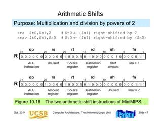
10.5 Logic and Shift Operations
Conceptually, shifts can be implemented by multiplexing
Figure 10.15 Multiplexer-based logical shifting unit.
Multiplexer
0 1 2 31 32 33 62 63
5
6
Right’Left
Shift amount 0, x[31, 1]
x[31, 0]
00, x[30, 2]
00...0, x[31]
x[31, 0]
x[30, 0], 0
x[1, 0], 00...0
x[0], 00...0
. . . . . .
32
32 32
32
32
32
32
32
32
6-bit code specifying
shift direction & amount
Right-shifted
values
Left-shifted
values](https://image.slidesharecdn.com/f37-book-intarch-pres-pt3-230913163318-64bba6b0/85/CA-ppt-46-320.jpg)
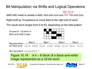
![Oct. 2014 Computer Architecture, The Arithmetic/Logic Unit Slide 48
Practical Shifting in Multiple Stages
Figure 10.17 Multistage shifting in a barrel shifter.
2
0, x[31, 1]
x[31, 0]
x[30, 0], 0
32
0 1 2 3
32 32 32 32
0 0 No shift
0 1 Logical left
1 0 Logical right
1 1 Arith right
x[31], x[31, 1]
Multiplexer
2
0 1 2 3
(0 or 4)-bit shift
2
0 1 2 3
(0 or 2)-bit shift
2
0 1 2 3
(0 or 1)-bit shift
(a) Single-bit shifter (b) Shifting by up to 7 bits
y[31, 0]
z[31, 0]](https://image.slidesharecdn.com/f37-book-intarch-pres-pt3-230913163318-64bba6b0/85/CA-ppt-48-320.jpg)
![Oct. 2014 Computer Architecture, The Arithmetic/Logic Unit Slide 63
shamu: move $v0,$zero # initialize Hi to 0
move $vl,$zero # initialize Lo to 0
addi $t2,$zero,32 # init repetition counter to 32
mloop: move $t0,$zero # set c-out to 0 in case of no add
move $t1,$a1 # copy ($a1) into $t1
srl $a1,1 # halve the unsigned value in $a1
subu $t1,$t1,$a1 # subtract ($a1) from ($t1) twice to
subu $t1,$t1,$a1 # obtain LSB of ($a1), or y[j], in $t1
beqz $t1,noadd # no addition needed if y[j] = 0
addu $v0,$v0,$a0 # add x to upper part of z
sltu $t0,$v0,$a0 # form carry-out of addition in $t0
noadd: move $t1,$v0 # copy ($v0) into $t1
srl $v0,1 # halve the unsigned value in $v0
subu $t1,$t1,$v0 # subtract ($v0) from ($t1) twice to
subu $t1,$t1,$v0 # obtain LSB of Hi in $t1
sll $t0,$t0,31 # carry-out converted to 1 in MSB of $t0
addu $v0,$v0,$t0 # right-shifted $v0 corrected
srl $v1,1 # halve the unsigned value in $v1
sll $t1,$t1,31 # LSB of Hi converted to 1 in MSB of $t1
addu $v1,$v1,$t1 # right-shifted $v1 corrected
addi $t2,$t2,-1 # decrement repetition counter by 1
bne $t2,$zero,mloop # if counter > 0, repeat multiply loop
jr $ra # return to the calling program
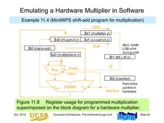
Multiplication When There Is No Multiply Instruction
Example 11.4 (MiniMIPS shift-add program for multiplication)](https://image.slidesharecdn.com/f37-book-intarch-pres-pt3-230913163318-64bba6b0/85/CA-ppt-63-320.jpg)
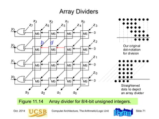
![Oct. 2014 Computer Architecture, The Arithmetic/Logic Unit Slide 74
shsdi: move $v0,$a2 # initialize Hi to ($a2)
move $vl,$a3 # initialize Lo to ($a3)
addi $t2,$zero,32 # initialize repetition counter to 32
dloop: slt $t0,$v0,$zero # copy MSB of Hi into $t0
sll $v0,$v0,1 # left-shift the Hi part of z
slt $t1,$v1,$zero # copy MSB of Lo into $t1
or $v0,$v0,$t1 # move MSB of Lo into LSB of Hi
sll $v1,$v1,1 # left-shift the Lo part of z
sge $t1,$v0,$a0 # quotient digit is 1 if (Hi) x,
or $t1,$t1,$t0 # or if MSB of Hi was 1 before shifting
sll $a1,$a1,1 # shift y to make room for new digit
or $a1,$a1,$t1 # copy y[k-j] into LSB of $a1
beq $t1,$zero,nosub # if y[k-j] = 0, do not subtract
subu $v0,$v0,$a0 # subtract divisor x from Hi part of z
nosub: addi $t2,$t2,-1 # decrement repetition counter by 1
bne $t2,$zero,dloop # if counter > 0, repeat divide loop
move $v1,$a1 # copy the quotient y into $v1
jr $ra # return to the calling program
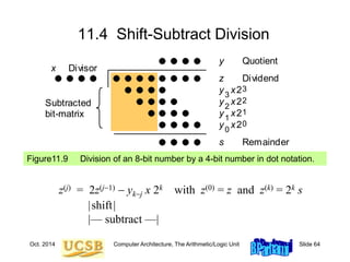
Division When There Is No Divide Instruction
Example 11.7 (MiniMIPS shift-subtract program for division)](https://image.slidesharecdn.com/f37-book-intarch-pres-pt3-230913163318-64bba6b0/85/CA-ppt-74-320.jpg)
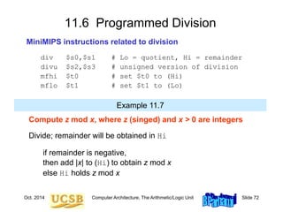
![Oct. 2014 Computer Architecture, The Arithmetic/Logic Unit Slide 78
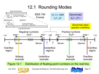
Figure 12.2 Two round-to-nearest-integer functions for x in [–4, 4].
Round-to-Nearest (Even)
rtnei(x)
–4
–3
–2
–1
x
–4 –3 –2 –1 4
3
2
1
4
3
2
1
rtni(x)
–4
–3
–2
–1
x
–4 –3 –2 –1 4
3
2
1
4
3
2
1
(a) Round to nearest even integer (b) Round to nearest integer](https://image.slidesharecdn.com/f37-book-intarch-pres-pt3-230913163318-64bba6b0/85/CA-ppt-78-320.jpg)
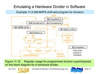
![Oct. 2014 Computer Architecture, The Arithmetic/Logic Unit Slide 79
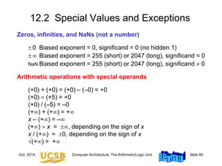
Figure 12.3 Two directed round-to-nearest-integer functions for x in [–4, 4].
Directed Rounding
(a) Round inward to nearest integer (b) Round upward to nearest integer
rutni(x)
–4
–3
–2
–1
x
–4 –3 –2 –1 4
3
2
1
4
3
2
1
ritni(x)
–4
–3
–2
–1
x
–4 –3 –2 –1 4
3
2
1
4
3
2
1](https://image.slidesharecdn.com/f37-book-intarch-pres-pt3-230913163318-64bba6b0/85/CA-ppt-79-320.jpg)

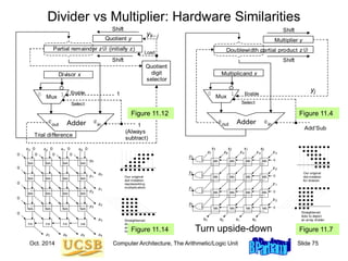
![Oct. 2014 Computer Architecture, The Arithmetic/Logic Unit Slide 89
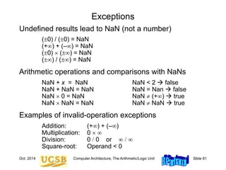
Floating-Point Data Transfers
MiniMIPS instructions for floating-point load, store, and move:
lwc1 $f8,40($s3) # load mem[40+($s3)] into $f8
swc1 $f8,A($s3) # store ($f8) into mem[A+($s3)]
mov.s $f0,$f8 # load $f0 with ($f8)
mov.d $f0,$f8 # load $f0,$f1 with ($f8,$f9)
mfc1 $t0,$f12 # load $t0 with ($f12)
mtc1 $f8,$t4 # load $f8 with ($t4)
Figure 12.9 Instructions for floating-point data movement in MiniMIPS.
0
1 1
0 0
x
0
1
1 0 0 0 0 0 0 0 0 0 0 0 0 0
0 1
0 0 0 0
0 0 0 0
31 25 20 15 0
Floating-point
instruction
s = 0
d = 1
Unused
op ex ft
F
fs fd
10 5
fn
Destination
register
mov.* = 6
Source
register
1 1
1 0 0
0
0
x
0
1
1 0 0 0 0 0 0 0 0 0 0 0 0 0
0 0 0
0 0
0 0 0
31 25 20 15 0
Floating-point
instruction
mfc1 = 0
mtc1 = 4
Unused
op rs rt
R
rd sh
10 5
fn
Destination
register
Source
register
Unused](https://image.slidesharecdn.com/f37-book-intarch-pres-pt3-230913163318-64bba6b0/85/CA-ppt-89-320.jpg)
![Oct. 2014 Computer Architecture, The Arithmetic/Logic Unit Slide 93
Error Control and Certifiable Arithmetic
Catastrophic cancellation in subtracting almost equal numbers:
Area of a needlelike triangle
A = [s(s – a)(s – b)(s – c)]1/2
Possible remedies
Carry extra precision in intermediate results (guard digits):
commonly used in calculators
Use alternate formula that does not produce cancellation errors
Certifiable arithmetic with intervals
A number is represented by its lower and upper bounds [xl, xu]
Example of arithmetic: [xl, xu] +interval [yl, yu] = [xl +fp yl, xu +fp yu]
a
b
c](https://image.slidesharecdn.com/f37-book-intarch-pres-pt3-230913163318-64bba6b0/85/CA-ppt-93-320.jpg)