Download as PDF, PPTX


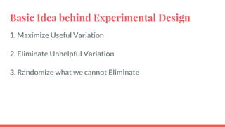


![Randomization & Linear Models
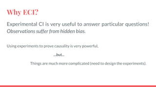
In all the below-mentioned cases, linear models (e.g. Linear Regression) can be
sufficient for the estimation of the expected causal effects, either entirely or under
conditions.
● Randomize one treatment
○ Binary Values
Coefficient on X: E[Y|X=1]-E[Y|X=0]
○ Discrete Values
Coefficients on X: E[Y|X=x]-E[Y|X=0] //for all x
● Randomize multiple treatments
E[Y|do(X=x,Z=z)] = μ + fX
(x) + fZ
(z) + fXZ
(x,z) //only if levels of X and Z are discrete](https://image.slidesharecdn.com/experimentalcausalinference-161115204924/85/Experimental-Causal-Inference-18-320.jpg)


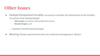
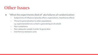

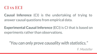
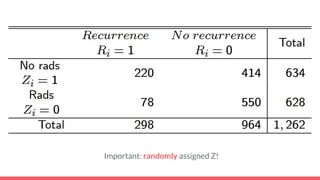
The document discusses experimental causal inference and key concepts in experimental design. It defines causal inference as trying to answer causal questions from data, and experimental causal inference as doing so using experiments rather than observations. The basic ideas of experimental design are outlined as maximizing useful variation, eliminating unhelpful variation, and randomizing what cannot be eliminated. Randomization is described as the key to ensuring treatment groups are statistically equivalent. Some open issues discussed include types of randomization, choice of treatment levels, and other challenges like multiple variables, blocking, and limitations of randomization.


![[DSC Europe 25] Marcos Heidemann - Beyond the Hype: Making AI Coding Assistan...](https://cdn.slidesharecdn.com/ss_thumbnails/eexkhvldrjsopspdjbur-marcos-heidemann-beyond-the-hype-getting-real-value-out-of-ai-assisted-coding-260121115910-7e9d41ec-thumbnail.jpg?width=640&height=640&fit=bounds)


![[DSC Europe 25] Srdj Stanisic - Local and Private AI in UX.pdf](https://cdn.slidesharecdn.com/ss_thumbnails/vwmetykqmztgmokmmkfa-3-srdjan-stanisic-local-and-small-ai-in-ux-260120105855-55a31869-thumbnail.jpg?width=640&height=640&fit=bounds)

![[DSC Europe 25] Tamas Srancsik - How To Teach Your AI Football? An Argument f...](https://cdn.slidesharecdn.com/ss_thumbnails/bcjh1m9xtbosv20ucftb-tamas-srancsik-how-to-teach-your-ai-football-260121115910-08b53e9e-thumbnail.jpg?width=640&height=640&fit=bounds)

![[DSC Europe 25] Milos Belcevic - Product Professional's Journey to Full-Stack...](https://cdn.slidesharecdn.com/ss_thumbnails/1zovd6fgsycdg4wvgvls-milos-belcevic-product-professionals-journey-to-full-stack-product-developer-260123083019-d993120d-thumbnail.jpg?width=640&height=640&fit=bounds)
