Exercise 14
Understanding Simple Linear Regression
Statistical Technique in Review
In nursing practice, the ability to predict future events or outcomes is crucial, and researchers calculate and report linear regression results as a basis for making these predictions.
Linear regression
provides a means to estimate or predict the value of a dependent variable based on the value of one or more independent variables. The regression equation is a mathematical expression of a causal proposition emerging from a theoretical framework. The linkage between the theoretical statement and the equation is made prior to data collection and analysis. Linear regression is a statistical method of estimating the expected value of one variable,
y
, given the value of another variable,
x
. The focus of this exercise is
simple linear regression
, which involves the use of one independent variable,
x
, to predict one dependent variable,
y
.
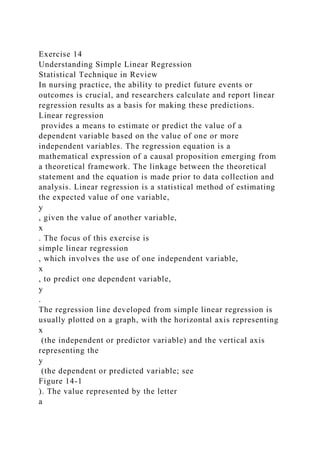
The regression line developed from simple linear regression is usually plotted on a graph, with the horizontal axis representing
x
(the independent or predictor variable) and the vertical axis representing the
y
(the dependent or predicted variable; see
Figure 14-1
). The value represented by the letter
a
is referred to as the
y
intercept, or the point where the regression line crosses or intercepts the
y
-axis. At this point on the regression line,
x
= 0. The value represented by the letter
b
is referred to as the slope, or the coefficient of
x
. The slope determines the direction and angle of the regression line within the graph. The slope expresses the extent to which
y
changes for every one-unit change in
x
. The score on variable
y
(dependent variable) is predicted from the subject's known score on variable
x
(independent variable). The predicted score or estimate is referred to as
Ŷ
(expressed as
y
-hat) (
Cohen, 1988
;
Grove, Burns, & Gray, 2013
;
Zar, 2010
).
FIGURE 14-1
GRAPH OF A SIMPLE LINEAR REGRESSION LINE
140
Simple linear regression is an effort to explain the dynamics within a scatterplot (see
Exercise 11
) by drawing a straight line through the plotted scores. No single regression line can be used to predict, with complete accuracy, every
y
value from every
x
value. However, the purpose of the regression equation is to develop the line to allow the highest degree of prediction possible, the
line of best fit
. The procedure for developing the line of best fit is the
method of least squares
. If the data were perfectly correlated, all data points would fall along the straight line or line of best fit. However, not all data points fall on the line of best fit in studies, but the line of best fit provides the best equation for the values of
y
to be predicted by locating the intersection of points on the line for any given value of
x
.
The algebraic equation for the regression line of best fit is
y
=
bx
+
a
, where:
y
=
dependent
variable
(
outcome
)
x
=
independen.
Exercise 29Calculating Simple Linear RegressionSimple linear reg.docxAlleneMcclendon878
Exercise 29
Calculating Simple Linear Regression
Simple linear regression
is a procedure that provides an estimate of the value of a dependent variable (outcome) based on the value of an independent variable (predictor). Knowing that estimate with some degree of accuracy, we can use regression analysis to predict the value of one variable if we know the value of the other variable (
Cohen & Cohen, 1983
). The regression equation is a mathematical expression of the influence that a predictor has on a dependent variable, based on some theoretical framework. For example, in
Exercise 14
,
Figure 14-1
illustrates the linear relationship between gestational age and birth weight. As shown in the scatterplot, there is a strong positive relationship between the two variables. Advanced gestational ages predict higher birth weights.
A regression equation can be generated with a data set containing subjects'
x
and
y
values. Once this equation is generated, it can be used to predict future subjects'
y
values, given only their
x
values. In simple or bivariate regression, predictions are made in cases with two variables. The score on variable
y
(dependent variable, or outcome) is predicted from the same subject's known score on variable
x
(independent variable, or predictor).
Research Designs Appropriate for Simple Linear Regression
Research designs that may utilize simple linear regression include any associational design (
Gliner et al., 2009
). The variables involved in the design are attributional, meaning the variables are characteristics of the participant, such as health status, blood pressure, gender, diagnosis, or ethnicity. Regardless of the nature of variables, the dependent variable submitted to simple linear regression must be measured as continuous, at the interval or ratio level.
Statistical Formula and Assumptions
Use of simple linear regression involves the following assumptions (
Zar, 2010
):
1.
Normal distribution of the dependent (
y
) variable
2.
Linear relationship between
x
and
y
3.
Independent observations
4.
No (or little) multicollinearity
5.
Homoscedasticity
320
Data that are
homoscedastic
are evenly dispersed both above and below the regression line, which indicates a linear relationship on a scatterplot. Homoscedasticity reflects equal variance of both variables. In other words, for every value of
x
, the distribution of
y
values should have equal variability. If the data for the predictor and dependent variable are not homoscedastic, inferences made during significance testing could be invalid (
Cohen & Cohen, 1983
;
Zar, 2010
). Visual examples of homoscedasticity and heteroscedasticity are presented in
Exercise 30
.
In simple linear regression, the dependent variable is continuous, and the predictor can be any scale of measurement; however, if the predictor is nominal, it must be correctly coded. Once the data are ready, the parameters
a
and
b
are computed to obtain a regression equatio.
Sara MaidaaHLTH 511 Research Methods Liberty University.docxanhlodge
Sara Maidaa
HLTH 511
Research Methods
Liberty University
Methods
Sample:
A population-based cross-sectional study was conducted on a sample of 20 primary school children, aged 4 to 15 years old.
Equipment:
Flexible inextensible tape: Task Force Hand Tools 25-foot tape measure.
Pediatric Height/Weight Scale
Measurements:
Weight and height were measured.
Written consent for physical examination was obtained from the parents.
All measurements were performed by trained research assistants, and under standard protocols.
Weight and height were measured twice to the nearest 0.1 cm and 0.1 kg, respectively, with children being barefoot and lightly dressed, and standing straight and immobile on the scale.
BMI was calculated as weight in kilograms divided by the square of height in meters (kg/m²).
Statistical Procedures:
Mean, median, standard deviation, minimum and maximum will be calculated for the sample. Data will be examined for outliers.
Pearson product moment correlation was used to determine the magnitude and significance of the relationship between food marketing and obesity in school children.
Hypotheses Being Tested:
Null Hypothesis: ρ (rho) =0 There is no significant relationship between food marketing and childhood obesity.
Alternative Hypothesis: ρ (rho) ≠0 There is a significant relationship between food marketing and childhood obesity.
Hypotheses tested at the 0.05 level of significance.
If a significant relationship between food marketing and childhood obesity is established then regression analysis was used to derive an equation to predict food marketing from obesity.
The Suitability of Arm Span as a Substitute Measurement for Height
HLTH 501
David M. Barton
Abstract
Many anthropometric equations rely on individual height. Accurate height is not obtainable when various skeletal abnormalities exist. Arm span is proposed as a possible substitute for height.
Thirteen subjects’ arm span and height were measured.
The Pearson R for arm span and height was 0.96 (p<0.05). Regression analysis was used to build and equation predicting height from arm span (Height = 0.8655 x Arm Span + 9.3368).
Results of this study show that arm span and height are strongly correlated and arm span can be used as a reliable predictor of height.
Introduction
In many medical, physiological, and human performance measurements the height of human subjects is used as a predictive and/or classification variable. Equations predicting Body Mass Index, pulmonary function, caloric expenditure, and body fat percentage are just a few of the many equations using height as a predictive variable.1
However, spinal curvature conditions such as kyphosis, scoliosis, lordosis, and kyphoscoliosis make it difficult to determine the correct height of the individual and thereby necessitating the need to identify a substitute anthropometric measurement.2
The need for an anthropometric measurement to serve as a substitute for height has long been recogn.
For this assignment, use the aschooltest.sav dataset.The dMerrileeDelvalle969
For this assignment, use the aschooltest.sav dataset.
The dataset consists of Reading, Writing, Math, Science, and Social Studies test scores for 200 students. Demographic data include gender, race, SES, school type, and program type.
Instructions:
Work with the aschooltest.sav datafile and respond to the following questions in a few sentences. Please submit your SPSS output either in your assignment or separately.
1. Identify an Independent and Dependent Variable (of your choice) and develop a hypothesis about what you expect to find. (
note: the IV is a grouping variable, which means it needs to have more than 2 categories and the DV is continuous)
2. Run Assumption tests for Normality and initial Homogeneity of Variance. What are your results?
3. Run the one-way ANOVA with the Levene test & Tukey post hoc test.
a. What are the results of the Levene test? What does this mean?
b. What are the results of the one-way ANOVA (use notation)? What does it mean?
c. Are post hoc tests necessary? If so, what are the results of those analyses?
4. How do your analyses address your hypotheses?
Is concentration of single parent families associated with reading scores?
Using the AECF state data, the regression below measures the effect of the state's percentage of single parent families on the percentage of 4th graders with below basic reading scores.
%belowbasicread = β0 + β1x%SPF + u
Stata Output
1) Please write out the regression equation using the coefficients in the table
2) Please provide an interpretation of the coefficient for SPF
3) How does the model fit?
4) What is the NULL hypothesis for a T test about a regression coefficient?
5) What is the ALTERNATE hypothesis for a T test about a regression coefficient?
6) Look at the p value for the coefficient SPF.
a) Report the p value
b) How many stars would it get if we used our standard convention?
* p ≤ .1 ** p ≤ .05 *** p ≤ .01
image1.png
Two-Variable (Bivariate) Regression
In the last unit, we covered scatterplots and correlation. Social scientists use these as descriptive tools for getting an idea about how our variables of interest are related. But these tools only get us so far. Regression analysis is the next step. Regression is by far the most used tool in social science research.
Simple regression analysis can tell us several things:
1. Regression can estimate the relationship between x and y in their
original units of measurement. To see why this is so useful, consider the example of infant mortality and median family income. Let’s say that a policymaker is interested in knowing how much of a change in median family income is needed to significantly reduce the infant mortality rate. Correlation cannot answer this question, but regression can.
2. Regression can tell us how well the independent variable (x) explains the dependent variable (y). The measure is called the
R square.
Simple Tw ...
16 USING LINEAR REGRESSION PREDICTING THE FUTURE16 MEDIA LIBRAR.docxhyacinthshackley2629
16 USING LINEAR REGRESSION PREDICTING THE FUTURE
16: MEDIA LIBRARY
Premium Videos
Core Concepts in Stats Video
· Linear Regression
Lightboard Lecture Video
· Multiple Regression
Time to Practice Video
· Chapter 16: Problem 2
Difficulty Scale
(as hard as they get!)
WHAT YOU WILL LEARN IN THIS CHAPTER
· Understanding how prediction works and how it can be used in the social and behavioral sciences
· Understanding how and why linear regression works when predicting one variable on the basis of another
· Judging the accuracy of predictions
· Understanding how multiple regression works and why it is useful
INTRODUCTION TO LINEAR REGRESSION
You’ve seen it all over the news—concern about obesity and how it affects work and daily life. A set of researchers in Sweden was interested in looking at how well mobility disability and/or obesity predicted job strain and whether social support at work can modify this association. The study included more than 35,000 participants, and differences in job strain mean scores were estimated using linear regression, the exact focus of what we are discussing in this chapter. The results found that level of mobile disability did predict job strain and that social support at work significantly modified the association among job strain, mobile disability, and obesity.
Want to know more? Go to the library or go online …
Norrback, M., De Munter, J., Tynelius, P., Ahlstrom, G., & Rasmussen, F. (2016). The association of mobility disability, weight status and job strain: A cross-sectional study. Scandinavian Journal of Public Health, 44, 311–319.
WHAT IS PREDICTION ALL ABOUT?
Here’s the scoop. Not only can you compute the degree to which two variables are related to one another (by computing a correlation coefficient as we did in Chapter 5), but you can also use these correlations to predict the value of one variable based on the value of another. This is a very special case of how correlations can be used, and it is a very powerful tool for social and behavioral sciences researchers.
The basic idea is to use a set of previously collected data (such as data on variables X and Y), calculate how correlated these variables are with one another, and then use that correlation and the knowledge of X to predict Y. Sound difficult? It’s not really, especially once you see it illustrated.
For example, a researcher collects data on total high school grade point average (GPA) and first-year college GPA for 400 students in their freshman year at the state university. He computes the correlation between the two variables. Then, he uses the techniques you’ll learn about later in this chapter to take a new set of high school GPAs and (knowing the relationship between high school GPA and first-year college GPA from the previous set of students) predict what first-year GPA should be for a new student who is just starting out. Pretty nifty, huh?
Here’s another example. A group of kindergarten teachers is interested in finding out how well ex.
16 USING LINEAR REGRESSION PREDICTING THE FUTURE16 MEDIA LIBRAR.docxnovabroom
16 USING LINEAR REGRESSION PREDICTING THE FUTURE
16: MEDIA LIBRARY
Premium Videos
Core Concepts in Stats Video
· Linear Regression
Lightboard Lecture Video
· Multiple Regression
Time to Practice Video
· Chapter 16: Problem 2
Difficulty Scale
(as hard as they get!)
WHAT YOU WILL LEARN IN THIS CHAPTER
· Understanding how prediction works and how it can be used in the social and behavioral sciences
· Understanding how and why linear regression works when predicting one variable on the basis of another
· Judging the accuracy of predictions
· Understanding how multiple regression works and why it is useful
INTRODUCTION TO LINEAR REGRESSION
You’ve seen it all over the news—concern about obesity and how it affects work and daily life. A set of researchers in Sweden was interested in looking at how well mobility disability and/or obesity predicted job strain and whether social support at work can modify this association. The study included more than 35,000 participants, and differences in job strain mean scores were estimated using linear regression, the exact focus of what we are discussing in this chapter. The results found that level of mobile disability did predict job strain and that social support at work significantly modified the association among job strain, mobile disability, and obesity.
Want to know more? Go to the library or go online …
Norrback, M., De Munter, J., Tynelius, P., Ahlstrom, G., & Rasmussen, F. (2016). The association of mobility disability, weight status and job strain: A cross-sectional study. Scandinavian Journal of Public Health, 44, 311–319.
WHAT IS PREDICTION ALL ABOUT?
Here’s the scoop. Not only can you compute the degree to which two variables are related to one another (by computing a correlation coefficient as we did in Chapter 5), but you can also use these correlations to predict the value of one variable based on the value of another. This is a very special case of how correlations can be used, and it is a very powerful tool for social and behavioral sciences researchers.
The basic idea is to use a set of previously collected data (such as data on variables X and Y), calculate how correlated these variables are with one another, and then use that correlation and the knowledge of X to predict Y. Sound difficult? It’s not really, especially once you see it illustrated.
For example, a researcher collects data on total high school grade point average (GPA) and first-year college GPA for 400 students in their freshman year at the state university. He computes the correlation between the two variables. Then, he uses the techniques you’ll learn about later in this chapter to take a new set of high school GPAs and (knowing the relationship between high school GPA and first-year college GPA from the previous set of students) predict what first-year GPA should be for a new student who is just starting out. Pretty nifty, huh?
Here’s another example. A group of kindergarten teachers is interested in finding out how well ex.
EXERCISE 23 PEARSON'S PRODUCT-MOMENT CORRELATION COEFFICIENT
STATISTICAL TECHNIQUE IN REVIEW
Many studies are conducted to identify relationships between or among variables. The correlational coefficient is the mathematical expression of
the relationship studied. Three common analysis techniques are used to examine relationships: Spearman Rank-Order Correlation or rho, Kendall's
Tau or tau, and the Pearson's Product-Moment Correlation Coefficient or r. Spearman and Kendall's Tau are used to examine relationships with
ordinal level data. Pearson's Correlation Coefficient is the most common correlational analysis technique used to examine the relationship
between two variables measured at the interval or ratio level.
Relationships are discussed in terms of direction and strength. The direction of the relationship is expressed as either positive or negative. A
positive or direct relationship exists when one variable increases as does the other variable increases, or when one variable decreases as the other
decreases. Conversely, a negative or inverse relationship exists when one variable increases and the other variable decreases. The strength of a
relationship is described as weak, moderate, or strong. Pearson's r is never greater than −1.00 or +1.00, so an r value of −1.00 or +1.00 indicates the
strongest possible relationship, either negative or positive, respectively. An r value of 0.00 indicates no relationship. To describe a relationship, the
labels weak (r < 0.3), moderate (r = 0.3 to 0.5), and strong (r > 0.5) are used in conjunction with both positive and negative values of r. Thus, the
strength of the negative relationships would be weak with r < −0.3, moderate with r = −0.3 to −0.5, and strong with r > −0.5 (Burns & Grove,
2007).
RESEARCH ARTICLE
Source: Keays, S. L., Bullock-Saxton, J. E., Newcombe, P., & Keays, A. C. (2003). The relationship between knee strength and functional
stability before and after anterior cruciate ligament reconstruction. Journal of Orthopedic Research, 21 (2), 231–7.
Introduction
Keays et al. (2003) conducted a correlational study to determine “the relationship between muscle strength and functional stability in 31 patients
pre- and postoperatively, following a unilateral anterior cruciate ligament rupture” (Keays et al., 2003, p. 231). The results of the study showed a
significant positive correlation between quadriceps strength indices and functional stability, both before and after surgery. No significant
relationship was demonstrated between hamstring strength indices 60°/s and functional stability, as presented in Table 5.
Relevant Study Results
“Patients with an unstable knee as a result of an anterior cruciate ligament (ACL) rupture rely heavily on muscle function around the joint to
maintain dynamic stability during functional activity. It is uncertain which muscles play the decisive role in functional stability or exactly which
aspect of muscle function is most ...
Running head COURSE PROJECT NCLEX Memorial Hospital .docxsusanschei
Running head: COURSE PROJECT: NCLEX Memorial Hospital 1
COURSE PROJECT: NCLEX Memorial Hospital 10
Introduction
This project aims to facilitate the improvement of the quality of healthcare services provided to individuals, families and communities at various age levels. Hence, this project used NCLEX Memorial Hospital, where over the past few days there has been a high level of infectious diseases. The dataset collected is from 60 patients whose age range is 35 to 76.
Classification of Variables
The quantitative variable is age. The qualitative variable is infectious diseases. Age is also a continuous variable as it can take on any value. A variable is any quantity that can be measured and whose value varies through the population and here the level of measurement is age, which we shall label a nominal measurement as numbers are used to classify the data.
The Measures of Center and the Measures of Variation
Themeasures of center are some of the most important descriptive statistics one might extrapolate. It helps give us an idea of what the "most" common, normal, or representative answers might be. Essentially, by getting an average, what you are really doing is calculating the "middle" of any group of observations. There are three measures of center that are most often used: Mean, Median and Mode. (NEDARC)
While measures of central tendency are used to estimate "normal" values of a dataset, measures of variation/dispersion are important for describing the spread of the data, or its variation around a central value. Two distinct samples may have the same mean or median, but completely different levels of variability, or vice versa. A proper description of a set of data should include both of these characteristics. There are various methods that can be used to measure the dispersion of a dataset, each with its own set of advantages and disadvantages. (Climate Data Library)
The Measures of Center and the Measures of Variation Calculations
Column1
Mean
61.81667
Standard Error
1.152127
Median
61.5
Mode
69
Standard Deviation
8.924337
Sample Variance
79.64379
Midrange
58.5
Range
41
Conclusion
By looking at the dataset we find that patients after the age of 50 and most likely 60 to be the most affected by infection diseases. Hence, there should be a prevention plan in place to reduce the number of infected or most likely to be affected by various viruses.
Course Project Phase 2
Introduction
The data in the accompanying spreadsheet records the ages of sixty (60) patients at NCLEX Memorial Hospital who, upon admission, were found to be suffering from ...
Introduction to statistical concepts (population, sample, sampling, central tendency, spread). Mainly aimed at language teachers in advanced studies programmes (e.g., Masters courses)
Explain in your own words why it is important to read a statistical .docxAlleneMcclendon878
Explain in your own words why it is important to read a statistical study carefully. Can you think of circumstance where it might be okay to misrepresent data?
Video Reflection 12 -
Do you think it is possible to create a study where there really is no bias sampling done? How would you manage to create one?
Video Reflection 13 -
What are your thoughts on statistics being misrepresented/ how does it make you feel? Why do you think the statistic are often presented in this way?
.
Explain how Matthew editedchanged Marks Gospel for each of the fol.docxAlleneMcclendon878
Explain how Matthew edited/changed Mark's Gospel for each of the following passages, and what reasons would he have had for doing that? What in Mk’s version was Mt trying to avoid – i.e., why he might have viewed Mk’s material as misleading, incorrect, or problematic? How did those changes contribute to Matthew’s overall message? How did that link up with other parts of Mt’s message?
Use both the following two sets of passages to support your claim, making use ONLY of the resources below, the Bible, textbooks and Module resources.
1. How did Matthew edit/change Mark 6:45-52 to produce Matthew 14:22-33 – and why?
2. How did Matthew edit/change Mark 9:2-10 to produce Matthew 17:1-13 – and why?
The paper should 350-750 words in length, double-spaced, and using MLA formatting for reference citations and bibliography. Submit the completed assignment to the appropriate Dropbox by
no later than Sunday 11:59 PM Eastern.
Resources for this paper:
See the ebook via SLU library:
New Testament History and Literature
by Martin (2012), pp. 83-88,105-108.
See the ebook via SLU library:
The Gospels
by Barton and Muddiman (2010), p. 53,56-57,102,109.
.
More Related Content
Similar to Exercise 14Understanding Simple Linear RegressionStatistical Tec.docx
For this assignment, use the aschooltest.sav dataset.The dMerrileeDelvalle969
For this assignment, use the aschooltest.sav dataset.
The dataset consists of Reading, Writing, Math, Science, and Social Studies test scores for 200 students. Demographic data include gender, race, SES, school type, and program type.
Instructions:
Work with the aschooltest.sav datafile and respond to the following questions in a few sentences. Please submit your SPSS output either in your assignment or separately.
1. Identify an Independent and Dependent Variable (of your choice) and develop a hypothesis about what you expect to find. (
note: the IV is a grouping variable, which means it needs to have more than 2 categories and the DV is continuous)
2. Run Assumption tests for Normality and initial Homogeneity of Variance. What are your results?
3. Run the one-way ANOVA with the Levene test & Tukey post hoc test.
a. What are the results of the Levene test? What does this mean?
b. What are the results of the one-way ANOVA (use notation)? What does it mean?
c. Are post hoc tests necessary? If so, what are the results of those analyses?
4. How do your analyses address your hypotheses?
Is concentration of single parent families associated with reading scores?
Using the AECF state data, the regression below measures the effect of the state's percentage of single parent families on the percentage of 4th graders with below basic reading scores.
%belowbasicread = β0 + β1x%SPF + u
Stata Output
1) Please write out the regression equation using the coefficients in the table
2) Please provide an interpretation of the coefficient for SPF
3) How does the model fit?
4) What is the NULL hypothesis for a T test about a regression coefficient?
5) What is the ALTERNATE hypothesis for a T test about a regression coefficient?
6) Look at the p value for the coefficient SPF.
a) Report the p value
b) How many stars would it get if we used our standard convention?
* p ≤ .1 ** p ≤ .05 *** p ≤ .01
image1.png
Two-Variable (Bivariate) Regression
In the last unit, we covered scatterplots and correlation. Social scientists use these as descriptive tools for getting an idea about how our variables of interest are related. But these tools only get us so far. Regression analysis is the next step. Regression is by far the most used tool in social science research.
Simple regression analysis can tell us several things:
1. Regression can estimate the relationship between x and y in their
original units of measurement. To see why this is so useful, consider the example of infant mortality and median family income. Let’s say that a policymaker is interested in knowing how much of a change in median family income is needed to significantly reduce the infant mortality rate. Correlation cannot answer this question, but regression can.
2. Regression can tell us how well the independent variable (x) explains the dependent variable (y). The measure is called the
R square.
Simple Tw ...
16 USING LINEAR REGRESSION PREDICTING THE FUTURE16 MEDIA LIBRAR.docxhyacinthshackley2629
16 USING LINEAR REGRESSION PREDICTING THE FUTURE
16: MEDIA LIBRARY
Premium Videos
Core Concepts in Stats Video
· Linear Regression
Lightboard Lecture Video
· Multiple Regression
Time to Practice Video
· Chapter 16: Problem 2
Difficulty Scale
(as hard as they get!)
WHAT YOU WILL LEARN IN THIS CHAPTER
· Understanding how prediction works and how it can be used in the social and behavioral sciences
· Understanding how and why linear regression works when predicting one variable on the basis of another
· Judging the accuracy of predictions
· Understanding how multiple regression works and why it is useful
INTRODUCTION TO LINEAR REGRESSION
You’ve seen it all over the news—concern about obesity and how it affects work and daily life. A set of researchers in Sweden was interested in looking at how well mobility disability and/or obesity predicted job strain and whether social support at work can modify this association. The study included more than 35,000 participants, and differences in job strain mean scores were estimated using linear regression, the exact focus of what we are discussing in this chapter. The results found that level of mobile disability did predict job strain and that social support at work significantly modified the association among job strain, mobile disability, and obesity.
Want to know more? Go to the library or go online …
Norrback, M., De Munter, J., Tynelius, P., Ahlstrom, G., & Rasmussen, F. (2016). The association of mobility disability, weight status and job strain: A cross-sectional study. Scandinavian Journal of Public Health, 44, 311–319.
WHAT IS PREDICTION ALL ABOUT?
Here’s the scoop. Not only can you compute the degree to which two variables are related to one another (by computing a correlation coefficient as we did in Chapter 5), but you can also use these correlations to predict the value of one variable based on the value of another. This is a very special case of how correlations can be used, and it is a very powerful tool for social and behavioral sciences researchers.
The basic idea is to use a set of previously collected data (such as data on variables X and Y), calculate how correlated these variables are with one another, and then use that correlation and the knowledge of X to predict Y. Sound difficult? It’s not really, especially once you see it illustrated.
For example, a researcher collects data on total high school grade point average (GPA) and first-year college GPA for 400 students in their freshman year at the state university. He computes the correlation between the two variables. Then, he uses the techniques you’ll learn about later in this chapter to take a new set of high school GPAs and (knowing the relationship between high school GPA and first-year college GPA from the previous set of students) predict what first-year GPA should be for a new student who is just starting out. Pretty nifty, huh?
Here’s another example. A group of kindergarten teachers is interested in finding out how well ex.
16 USING LINEAR REGRESSION PREDICTING THE FUTURE16 MEDIA LIBRAR.docxnovabroom
16 USING LINEAR REGRESSION PREDICTING THE FUTURE
16: MEDIA LIBRARY
Premium Videos
Core Concepts in Stats Video
· Linear Regression
Lightboard Lecture Video
· Multiple Regression
Time to Practice Video
· Chapter 16: Problem 2
Difficulty Scale
(as hard as they get!)
WHAT YOU WILL LEARN IN THIS CHAPTER
· Understanding how prediction works and how it can be used in the social and behavioral sciences
· Understanding how and why linear regression works when predicting one variable on the basis of another
· Judging the accuracy of predictions
· Understanding how multiple regression works and why it is useful
INTRODUCTION TO LINEAR REGRESSION
You’ve seen it all over the news—concern about obesity and how it affects work and daily life. A set of researchers in Sweden was interested in looking at how well mobility disability and/or obesity predicted job strain and whether social support at work can modify this association. The study included more than 35,000 participants, and differences in job strain mean scores were estimated using linear regression, the exact focus of what we are discussing in this chapter. The results found that level of mobile disability did predict job strain and that social support at work significantly modified the association among job strain, mobile disability, and obesity.
Want to know more? Go to the library or go online …
Norrback, M., De Munter, J., Tynelius, P., Ahlstrom, G., & Rasmussen, F. (2016). The association of mobility disability, weight status and job strain: A cross-sectional study. Scandinavian Journal of Public Health, 44, 311–319.
WHAT IS PREDICTION ALL ABOUT?
Here’s the scoop. Not only can you compute the degree to which two variables are related to one another (by computing a correlation coefficient as we did in Chapter 5), but you can also use these correlations to predict the value of one variable based on the value of another. This is a very special case of how correlations can be used, and it is a very powerful tool for social and behavioral sciences researchers.
The basic idea is to use a set of previously collected data (such as data on variables X and Y), calculate how correlated these variables are with one another, and then use that correlation and the knowledge of X to predict Y. Sound difficult? It’s not really, especially once you see it illustrated.
For example, a researcher collects data on total high school grade point average (GPA) and first-year college GPA for 400 students in their freshman year at the state university. He computes the correlation between the two variables. Then, he uses the techniques you’ll learn about later in this chapter to take a new set of high school GPAs and (knowing the relationship between high school GPA and first-year college GPA from the previous set of students) predict what first-year GPA should be for a new student who is just starting out. Pretty nifty, huh?
Here’s another example. A group of kindergarten teachers is interested in finding out how well ex.
EXERCISE 23 PEARSON'S PRODUCT-MOMENT CORRELATION COEFFICIENT
STATISTICAL TECHNIQUE IN REVIEW
Many studies are conducted to identify relationships between or among variables. The correlational coefficient is the mathematical expression of
the relationship studied. Three common analysis techniques are used to examine relationships: Spearman Rank-Order Correlation or rho, Kendall's
Tau or tau, and the Pearson's Product-Moment Correlation Coefficient or r. Spearman and Kendall's Tau are used to examine relationships with
ordinal level data. Pearson's Correlation Coefficient is the most common correlational analysis technique used to examine the relationship
between two variables measured at the interval or ratio level.
Relationships are discussed in terms of direction and strength. The direction of the relationship is expressed as either positive or negative. A
positive or direct relationship exists when one variable increases as does the other variable increases, or when one variable decreases as the other
decreases. Conversely, a negative or inverse relationship exists when one variable increases and the other variable decreases. The strength of a
relationship is described as weak, moderate, or strong. Pearson's r is never greater than −1.00 or +1.00, so an r value of −1.00 or +1.00 indicates the
strongest possible relationship, either negative or positive, respectively. An r value of 0.00 indicates no relationship. To describe a relationship, the
labels weak (r < 0.3), moderate (r = 0.3 to 0.5), and strong (r > 0.5) are used in conjunction with both positive and negative values of r. Thus, the
strength of the negative relationships would be weak with r < −0.3, moderate with r = −0.3 to −0.5, and strong with r > −0.5 (Burns & Grove,
2007).
RESEARCH ARTICLE
Source: Keays, S. L., Bullock-Saxton, J. E., Newcombe, P., & Keays, A. C. (2003). The relationship between knee strength and functional
stability before and after anterior cruciate ligament reconstruction. Journal of Orthopedic Research, 21 (2), 231–7.
Introduction
Keays et al. (2003) conducted a correlational study to determine “the relationship between muscle strength and functional stability in 31 patients
pre- and postoperatively, following a unilateral anterior cruciate ligament rupture” (Keays et al., 2003, p. 231). The results of the study showed a
significant positive correlation between quadriceps strength indices and functional stability, both before and after surgery. No significant
relationship was demonstrated between hamstring strength indices 60°/s and functional stability, as presented in Table 5.
Relevant Study Results
“Patients with an unstable knee as a result of an anterior cruciate ligament (ACL) rupture rely heavily on muscle function around the joint to
maintain dynamic stability during functional activity. It is uncertain which muscles play the decisive role in functional stability or exactly which
aspect of muscle function is most ...
Running head COURSE PROJECT NCLEX Memorial Hospital .docxsusanschei
Running head: COURSE PROJECT: NCLEX Memorial Hospital 1
COURSE PROJECT: NCLEX Memorial Hospital 10
Introduction
This project aims to facilitate the improvement of the quality of healthcare services provided to individuals, families and communities at various age levels. Hence, this project used NCLEX Memorial Hospital, where over the past few days there has been a high level of infectious diseases. The dataset collected is from 60 patients whose age range is 35 to 76.
Classification of Variables
The quantitative variable is age. The qualitative variable is infectious diseases. Age is also a continuous variable as it can take on any value. A variable is any quantity that can be measured and whose value varies through the population and here the level of measurement is age, which we shall label a nominal measurement as numbers are used to classify the data.
The Measures of Center and the Measures of Variation
Themeasures of center are some of the most important descriptive statistics one might extrapolate. It helps give us an idea of what the "most" common, normal, or representative answers might be. Essentially, by getting an average, what you are really doing is calculating the "middle" of any group of observations. There are three measures of center that are most often used: Mean, Median and Mode. (NEDARC)
While measures of central tendency are used to estimate "normal" values of a dataset, measures of variation/dispersion are important for describing the spread of the data, or its variation around a central value. Two distinct samples may have the same mean or median, but completely different levels of variability, or vice versa. A proper description of a set of data should include both of these characteristics. There are various methods that can be used to measure the dispersion of a dataset, each with its own set of advantages and disadvantages. (Climate Data Library)
The Measures of Center and the Measures of Variation Calculations
Column1
Mean
61.81667
Standard Error
1.152127
Median
61.5
Mode
69
Standard Deviation
8.924337
Sample Variance
79.64379
Midrange
58.5
Range
41
Conclusion
By looking at the dataset we find that patients after the age of 50 and most likely 60 to be the most affected by infection diseases. Hence, there should be a prevention plan in place to reduce the number of infected or most likely to be affected by various viruses.
Course Project Phase 2
Introduction
The data in the accompanying spreadsheet records the ages of sixty (60) patients at NCLEX Memorial Hospital who, upon admission, were found to be suffering from ...
Introduction to statistical concepts (population, sample, sampling, central tendency, spread). Mainly aimed at language teachers in advanced studies programmes (e.g., Masters courses)
Explain in your own words why it is important to read a statistical .docxAlleneMcclendon878
Explain in your own words why it is important to read a statistical study carefully. Can you think of circumstance where it might be okay to misrepresent data?
Video Reflection 12 -
Do you think it is possible to create a study where there really is no bias sampling done? How would you manage to create one?
Video Reflection 13 -
What are your thoughts on statistics being misrepresented/ how does it make you feel? Why do you think the statistic are often presented in this way?
.
Explain how Matthew editedchanged Marks Gospel for each of the fol.docxAlleneMcclendon878
Explain how Matthew edited/changed Mark's Gospel for each of the following passages, and what reasons would he have had for doing that? What in Mk’s version was Mt trying to avoid – i.e., why he might have viewed Mk’s material as misleading, incorrect, or problematic? How did those changes contribute to Matthew’s overall message? How did that link up with other parts of Mt’s message?
Use both the following two sets of passages to support your claim, making use ONLY of the resources below, the Bible, textbooks and Module resources.
1. How did Matthew edit/change Mark 6:45-52 to produce Matthew 14:22-33 – and why?
2. How did Matthew edit/change Mark 9:2-10 to produce Matthew 17:1-13 – and why?
The paper should 350-750 words in length, double-spaced, and using MLA formatting for reference citations and bibliography. Submit the completed assignment to the appropriate Dropbox by
no later than Sunday 11:59 PM Eastern.
Resources for this paper:
See the ebook via SLU library:
New Testament History and Literature
by Martin (2012), pp. 83-88,105-108.
See the ebook via SLU library:
The Gospels
by Barton and Muddiman (2010), p. 53,56-57,102,109.
.
Explain the degree to which media portrayal of crime relates to publ.docxAlleneMcclendon878
Explain the degree to which media portrayal of crime relates to public fear of crime and explain how.
Explain whether public fear of crime might influence individual behavior or not and explain how or how not.
Share an insight about whether media should be responsible or not for the portrayal of crime as it relates to public fear of crime.
2 Pages in APA Format
.
Explain the difference between genotype and phenotype. Give an examp.docxAlleneMcclendon878
Explain the difference between genotype and phenotype. Give an example of each and describe both in an account that relates to you personally, the
paper should be 2-3 pages in length (not counting the title and resources pages), APA style (no abstract required), and should be supported with appropriate citations.
.
Explain the history behind the Black Soldier of the Civil War In t.docxAlleneMcclendon878
Explain the history behind the Black Soldier of the Civil War
In this forum look beyond the book for information on specific units, soldiers and even the reasons for why Lincoln allowed the African American to service in the war.
Soldiers - the trained and untrained
Initial post of at least 300 words due by Friday.
Darlene Hine, William Hine, and Stanley Harrold.
The African-American Odyssey: Volume I, 6th ed. New Jersey: Pearson 2014.
.
Explain the fundamental reasons why brands do not exist in isolation.docxAlleneMcclendon878
Explain the fundamental reasons why brands do not exist in isolation but do exist in larger environments that include other brands. Provide two (2) specific recommendations or solutions that can help a health care facility improve patient satisfaction.
Assess the value of Lederer and Hill's Brand Portfolio Molecule when used to understand brand relationships. Provide at least two (2) specific examples of strategic or tactical initiatives within a health care organization.
.
Explain the difference between hypothetical and categorical imperati.docxAlleneMcclendon878
Explain the difference between hypothetical and categorical imperatives. How might this distinction be used to explore the practice of correctional facilities placing violent prisoners in solitary confinement?
Please use in-text citations and provide references. Seeking a one-page response.
.
Explain in 100 words provide exampleThe capital budgeting decisi.docxAlleneMcclendon878
Explain in 100 words provide example
The capital budgeting decision techniques that we've discussed all have strengths and weaknesses, but they do comprise the most popular rules for valuing projects. Valuing entire businesses, on the other hand, requires that some adjustments be made to various pieces of these methodologies. For example, one alternative to NPV used quite frequently for valuing firms is called Adjusted Present Value (APV).
What is APV, and how does it differ from NPV?
.
Explain how Supreme Court decisions influenced the evolution of the .docxAlleneMcclendon878
Explain how Supreme Court decisions influenced the evolution of the death penalty.
Explain the financial impact of the death penalty on society. Include at least one specific cost associated with the death penalty.
Explain the social impact of the death penalty on society. Provide examples and use Learning Resources to support your statements. 2 pages in APA format
.
Explain how an offender is classified according to risk when he or s.docxAlleneMcclendon878
Explain how an offender is classified according to risk when he or she is placed on probation or parole. Include how static and dynamic factors are taken into account by the supervising officer when both determining the level of supervision an offender needs and in developing the case-supervision plan for the offender. Include a discussion on the various levels of probation/parole supervision and the amount of surveillance and contact with the offender involved with each level. Do you agree or disagree with how often probation and parole officers have contact with high-risk offenders? Make sure to support your opinion.
.
Explain a lesson plan. Describe the different types of information.docxAlleneMcclendon878
Explain a lesson plan. Describe the different types of information found in a detailed lesson plan. Include in your discussion a design document and its usefulness. (A Minimum 525 Words)
Reference:
Noe, R. A. (2013). Employee training and development (6th ed.). New York, NY: McGraw-Hill.
.
explain the different roles of basic and applied researchdescribe .docxAlleneMcclendon878
explain the different roles of basic and applied research
describe the different criteria for success of basic and applied research
explain why government policymakers seem to prefer applied research
describe how basic research reflects liberal democratic values
Over fifty years ago, Vannevar Bush released his enormously influential report, Science, the Endless Frontier, which asserted a dichotomy between basic and applied science. This view was at the core of the compact between government and science that led to the golden age of scientific research after World War II—a compact that is currently under severe stress. In this book, Donald Stokes challenges Bush’s view and maintains that we can only rebuild the relationship between government and the scientific community when we understand what is wrong with that view.
Stokes begins with an analysis of the goals of understanding and use in scientific research. He recasts the widely accepted view of the tension between understanding and use, citing as a model case the fundamental yet use-inspired studies by which Louis Pasteur laid the foundations of microbiology a century ago. Pasteur worked in the era of the “second industrial revolution,” when the relationship between basic science and technological change assumed its modern form. Over subsequent decades, technology has been increasingly science-based. But science has been increasingly technology-based–with the choice of problems and the conduct of research often inspired by societal needs. An example is the work of the quantum-effects physicists who are probing the phenomena revealed by the miniaturization of semiconductors from the time of the transistor’s discovery after World War II.
On this revised, interactive view of science and technology, Stokes builds a convincing case that by recognizing the importance of use-inspired basic research we can frame a new compact between science and government. His conclusions have major implications for both the scientific and policy communities and will be of great interest to those in the broader public who are troubled by the current role of basic science in American democracy.
Why the distinction between basic (theoretical) and applied
(practical) research is important in the politics of science
.
Explain the basics of inspirational and emotion-provoking communicat.docxAlleneMcclendon878
Explain the basics of inspirational and emotion-provoking communication.
Explain the key features of a power-oriented linguistic style.
Explain the six basic principles of persuasion.
Evaluate basic approaches to resolving conflict and negotiating.
Choose one of the above topics
1 Paragraph
1 APA citation
.
Explain how leaders develop through self-awareness and self-discipli.docxAlleneMcclendon878
Explain how leaders develop through self-awareness and self-discipline.
Explain how leaders develop through education, experience, and mentoring.
Explain and classify the nature of leadership development programs.
Explain the nature of leadership succession and the importance of this practice.
3-4 page paper
APA Citation
4 sources
.
Explain five ways that you can maintain professionalism in the meeti.docxAlleneMcclendon878
Explain five ways that you can maintain professionalism in the meeting and convention planning industry.
1.
Order of precedence
2.
Titles and styles of address
3.
Invitations
4.
Flags
5.
Religious, cultural and ritual observations
.
Explain security awareness and its importance.Your response should.docxAlleneMcclendon878
Explain security awareness and its importance.
Your response should be at least 200 words in length.
Explain network and data privacy policies.
Your response should be at least 200 words in length.
Explain the different security positions within information security.
Your response should be at least 200 words in length.
Explain what a security incident response team handles.
Your response should be at least 200 words in length.
.
Experimental Design AssignmentYou were given an Aedesaegyp.docxAlleneMcclendon878
Experimental Design Assignment
You were given an
Aedes
aegypti
gene of unknown function. Using Blast you were able to find the homologs of your gene. You have done research regarding the function of the homologs. Using this information:
A.Construct
a hypothesis
Give a hypothesis on the function of your gene SHAKER is in Aedesaegypti.
B.Design
an experiment to test your hypothesis.
Include a
labeled
sketch and written summary of experiment. (
include drawing of all conditions
, negative/positive etc)
C. Variables
List the Dependent and Independent
List Control variable
List a Positive and /or Negative controls
D.
Create a
data
set
and figure
Create a graph that clearly conveys to the reader what your experiment is about.
F.Interpretation
Give an interpretation of the possible meaning of your data. (although this isn’t conclusive since we are not doing statistics) . Does it align with your hypothesis?
G.Self-critique
and follow-up questions:
Why might your conclusion be wrong, what other questions do you have.
.
Expand your website plan.Select at least three interactive fea.docxAlleneMcclendon878
Expand
your website plan.
Select
at least three interactive features that could be added to your site.
Identify
the following:
What purpose would each feature serve for your site and its visitors?
How would you construct these features?
Note
: The form created in the next individual activity, "Individual: Refine and Finalize Website" can be included as one of the interactive features.
.
Exercise 7 Use el pronombre y la forma correcta del verbo._.docxAlleneMcclendon878
Exercise 7: Use el pronombre y la forma correcta del verbo.
____________________________
gustar faltar quedar molestar
encantar fascinar interesar
____________________________
1. A mi ______ __________ la poesía romántica.
2. A nosotros ______ ________ estudiar lenguas extranjeras.
3. A las muchachas ______ _______ la música de Julio Iglesias.
4. A Juan y a Ramón ______ ___________ practicar los deportes.
5. A ti no _____ _________ el café.
6. A la profesora no ______ ________ preparar los exámenes.
7. Al consejero _____ ____________ los estudiantes.
8. A los atletas ____ ___________ el gimnasio.
9. Tenemos $500 y pagamos $350 por la matricula. ___ ___________ $150.
10. A los doctores ____ ________ la medicina.
11. A nosotros ____ ________ las pizzas.
12. A ellos ____ __________ la violencia.
13. En la Argentina bailan mucho. A ellos ____ ______ el tango.
14. Nosotros deseamos buscar el vocabulario. ____ __________ un diccionario.
15. Uds. desean llamar a los amigos. ____ ________ un teléfono.
16. A los estudiantes ________ ________ las vacaciones.
17. A mí ________ _________ los actores.
18. A Ud. _________ ____________ solamente diez dólares.
19. A Alberto y a Juan _______ ____________ el béisbol.
20. A ti _______ ____________ trabajar.
21. A Marisa _____ _____________ la música popular.
22. Nosotros terminamos una clase de español y ahora, _________ _______ dos clases
de español.
.
Exercise 21-8 (Part Level Submission)The following facts pertain.docxAlleneMcclendon878
Exercise 21-8 (Part Level Submission)
The following facts pertain to a noncancelable lease agreement between Windsor Leasing Company and Sheridan Company, a lessee.
Inception date:
May 1, 2017
Annual lease payment due at the beginning of
each year, beginning with May 1, 2017
$21,737.01
Bargain-purchase option price at end of lease term
$3,800
Lease term
5
years
Economic life of leased equipment
10
years
Lessor’s cost
$68,000
Fair value of asset at May 1, 2017
$93,000
Lessor’s implicit rate
10
%
Lessee’s incremental borrowing rate
10
%
The collectibility of the lease payments is reasonably predictable, and there are no important uncertainties surrounding the costs yet to be incurred by the lessor. The lessee assumes responsibility for all executory costs.
Click here to view factor tables
(c)
Your answer is partially correct. Try again.
Prepare a lease amortization schedule for Sheridan Company for the 5-year lease term.
(Round present value factor calculations to 5 decimal places, e.g. 1.25125 and Round answers to 2 decimal places, e.g. 15.25.)
SHERIDAN COMPANY (Lessee)
Lease Amortization Schedule
Date
Annual Lease Payment Plus
BPO
Interest on
Liability
Reduction of Lease
Liability
Lease Liability
5/1/17
$
[removed]
[removed]
[removed]
[removed]
[removed]
[removed]
(To record depreciation.)
[removed]
[removed]
[removed]
[removed]
[removed]
[removed]
(To record interest.)
1/1/18
[removed]
[removed]
[removed]
[removed]
[removed]
[removed]
[removed]
[removed]
[removed]
(To record second payament.)
Question 27
Pearl Corporation manufactures replicators. On January 1, 2017, it leased to Althaus Company a replicator that had cost $100,000 to manufacture. The lease agreement covers the 5-year useful life of the replicator and requires 5 equal annual rentals of $40,200 payable each January 1, beginning January 1, 2017. An interest rate of 12% is implicit in the lease agreement. Collectibility of the rentals is reasonably assured, and there are no important uncertainties concerning costs.
Prepare Pearl’s January 1, 2017, journal entries.
(Credit account titles are automatically indented when amount is entered. Do not indent manually. If no entry is required, select "No Entry" for the account titles and enter 0 for the amounts. Round present value factor calculations to 5 decimal places, e.g. 1.25124 and the final answer to 0 decimal places e.g. 58,971
.
)
Click here to view factor tables
Date
Account Titles and Explanation
Debit
Credit
January 1, 2017
[removed]
[removed]
[removed]
[removed]
[removed]
[removed]
(To record the lease.)
January 1, 2017
[removed]
[removed]
[removed]
[removed]
[removed]
[removed]
(To record cost.)
January 1, 2017
[removed]
[removed]
[removed]
[removed]
[removed]
[removed]
(To record first lease payment.)
6 years ago
16.01.2017
8
Report Issue
Answer
(
0
)
Bids
(
0
)
other Questions
(
10
)
what can i bring to class that symbolizes growth and change
calculate it.
Synthetic Fiber Construction in lab .pptxPavel ( NSTU)
Synthetic fiber production is a fascinating and complex field that blends chemistry, engineering, and environmental science. By understanding these aspects, students can gain a comprehensive view of synthetic fiber production, its impact on society and the environment, and the potential for future innovations. Synthetic fibers play a crucial role in modern society, impacting various aspects of daily life, industry, and the environment. ynthetic fibers are integral to modern life, offering a range of benefits from cost-effectiveness and versatility to innovative applications and performance characteristics. While they pose environmental challenges, ongoing research and development aim to create more sustainable and eco-friendly alternatives. Understanding the importance of synthetic fibers helps in appreciating their role in the economy, industry, and daily life, while also emphasizing the need for sustainable practices and innovation.
How to Create Map Views in the Odoo 17 ERPCeline George
The map views are useful for providing a geographical representation of data. They allow users to visualize and analyze the data in a more intuitive manner.
How to Split Bills in the Odoo 17 POS ModuleCeline George
Bills have a main role in point of sale procedure. It will help to track sales, handling payments and giving receipts to customers. Bill splitting also has an important role in POS. For example, If some friends come together for dinner and if they want to divide the bill then it is possible by POS bill splitting. This slide will show how to split bills in odoo 17 POS.
Model Attribute Check Company Auto PropertyCeline George
In Odoo, the multi-company feature allows you to manage multiple companies within a single Odoo database instance. Each company can have its own configurations while still sharing common resources such as products, customers, and suppliers.
Unit 8 - Information and Communication Technology (Paper I).pdfThiyagu K
This slides describes the basic concepts of ICT, basics of Email, Emerging Technology and Digital Initiatives in Education. This presentations aligns with the UGC Paper I syllabus.
We all have good and bad thoughts from time to time and situation to situation. We are bombarded daily with spiraling thoughts(both negative and positive) creating all-consuming feel , making us difficult to manage with associated suffering. Good thoughts are like our Mob Signal (Positive thought) amidst noise(negative thought) in the atmosphere. Negative thoughts like noise outweigh positive thoughts. These thoughts often create unwanted confusion, trouble, stress and frustration in our mind as well as chaos in our physical world. Negative thoughts are also known as “distorted thinking”.
Welcome to TechSoup New Member Orientation and Q&A (May 2024).pdfTechSoup
In this webinar you will learn how your organization can access TechSoup's wide variety of product discount and donation programs. From hardware to software, we'll give you a tour of the tools available to help your nonprofit with productivity, collaboration, financial management, donor tracking, security, and more.
Operation “Blue Star” is the only event in the history of Independent India where the state went into war with its own people. Even after about 40 years it is not clear if it was culmination of states anger over people of the region, a political game of power or start of dictatorial chapter in the democratic setup.
The people of Punjab felt alienated from main stream due to denial of their just demands during a long democratic struggle since independence. As it happen all over the word, it led to militant struggle with great loss of lives of military, police and civilian personnel. Killing of Indira Gandhi and massacre of innocent Sikhs in Delhi and other India cities was also associated with this movement.
The Roman Empire A Historical Colossus.pdfkaushalkr1407
The Roman Empire, a vast and enduring power, stands as one of history's most remarkable civilizations, leaving an indelible imprint on the world. It emerged from the Roman Republic, transitioning into an imperial powerhouse under the leadership of Augustus Caesar in 27 BCE. This transformation marked the beginning of an era defined by unprecedented territorial expansion, architectural marvels, and profound cultural influence.
The empire's roots lie in the city of Rome, founded, according to legend, by Romulus in 753 BCE. Over centuries, Rome evolved from a small settlement to a formidable republic, characterized by a complex political system with elected officials and checks on power. However, internal strife, class conflicts, and military ambitions paved the way for the end of the Republic. Julius Caesar’s dictatorship and subsequent assassination in 44 BCE created a power vacuum, leading to a civil war. Octavian, later Augustus, emerged victorious, heralding the Roman Empire’s birth.
Under Augustus, the empire experienced the Pax Romana, a 200-year period of relative peace and stability. Augustus reformed the military, established efficient administrative systems, and initiated grand construction projects. The empire's borders expanded, encompassing territories from Britain to Egypt and from Spain to the Euphrates. Roman legions, renowned for their discipline and engineering prowess, secured and maintained these vast territories, building roads, fortifications, and cities that facilitated control and integration.
The Roman Empire’s society was hierarchical, with a rigid class system. At the top were the patricians, wealthy elites who held significant political power. Below them were the plebeians, free citizens with limited political influence, and the vast numbers of slaves who formed the backbone of the economy. The family unit was central, governed by the paterfamilias, the male head who held absolute authority.
Culturally, the Romans were eclectic, absorbing and adapting elements from the civilizations they encountered, particularly the Greeks. Roman art, literature, and philosophy reflected this synthesis, creating a rich cultural tapestry. Latin, the Roman language, became the lingua franca of the Western world, influencing numerous modern languages.
Roman architecture and engineering achievements were monumental. They perfected the arch, vault, and dome, constructing enduring structures like the Colosseum, Pantheon, and aqueducts. These engineering marvels not only showcased Roman ingenuity but also served practical purposes, from public entertainment to water supply.
This is a presentation by Dada Robert in a Your Skill Boost masterclass organised by the Excellence Foundation for South Sudan (EFSS) on Saturday, the 25th and Sunday, the 26th of May 2024.
He discussed the concept of quality improvement, emphasizing its applicability to various aspects of life, including personal, project, and program improvements. He defined quality as doing the right thing at the right time in the right way to achieve the best possible results and discussed the concept of the "gap" between what we know and what we do, and how this gap represents the areas we need to improve. He explained the scientific approach to quality improvement, which involves systematic performance analysis, testing and learning, and implementing change ideas. He also highlighted the importance of client focus and a team approach to quality improvement.
The French Revolution, which began in 1789, was a period of radical social and political upheaval in France. It marked the decline of absolute monarchies, the rise of secular and democratic republics, and the eventual rise of Napoleon Bonaparte. This revolutionary period is crucial in understanding the transition from feudalism to modernity in Europe.
For more information, visit-www.vavaclasses.com
The French Revolution Class 9 Study Material pdf free download
Exercise 14Understanding Simple Linear RegressionStatistical Tec.docx
1. Exercise 14
Understanding Simple Linear Regression
Statistical Technique in Review
In nursing practice, the ability to predict future events or
outcomes is crucial, and researchers calculate and report linear
regression results as a basis for making these predictions.
Linear regression
provides a means to estimate or predict the value of a
dependent variable based on the value of one or more
independent variables. The regression equation is a
mathematical expression of a causal proposition emerging from
a theoretical framework. The linkage between the theoretical
statement and the equation is made prior to data collection and
analysis. Linear regression is a statistical method of estimating
the expected value of one variable,
y
, given the value of another variable,
x
. The focus of this exercise is
simple linear regression
, which involves the use of one independent variable,
x
, to predict one dependent variable,
y
.
The regression line developed from simple linear regression is
usually plotted on a graph, with the horizontal axis representing
x
(the independent or predictor variable) and the vertical axis
representing the
y
(the dependent or predicted variable; see
Figure 14-1
). The value represented by the letter
a
2. is referred to as the
y
intercept, or the point where the regression line crosses or
intercepts the
y
-axis. At this point on the regression line,
x
= 0. The value represented by the letter
b
is referred to as the slope, or the coefficient of
x
. The slope determines the direction and angle of the regression
line within the graph. The slope expresses the extent to which
y
changes for every one-unit change in
x
. The score on variable
y
(dependent variable) is predicted from the subject's known
score on variable
x
(independent variable). The predicted score or estimate is
referred to as
Ŷ
(expressed as
y
-hat) (
Cohen, 1988
;
Grove, Burns, & Gray, 2013
;
Zar, 2010
).
FIGURE 14-1
3. GRAPH OF A SIMPLE LINEAR REGRESSION LINE
140
Simple linear regression is an effort to explain the dynamics
within a scatterplot (see
Exercise 11
) by drawing a straight line through the plotted scores. No
single regression line can be used to predict, with complete
accuracy, every
y
value from every
x
value. However, the purpose of the regression equation is to
develop the line to allow the highest degree of prediction
possible, the
line of best fit
. The procedure for developing the line of best fit is the
method of least squares
. If the data were perfectly correlated, all data points would fall
along the straight line or line of best fit. However, not all data
points fall on the line of best fit in studies, but the line of best
fit provides the best equation for the values of
y
to be predicted by locating the intersection of points on the line
for any given value of
x
.
The algebraic equation for the regression line of best fit is
y
=
bx
+
a
, where:
y
=
dependent
7. -axis represents Gestational Age in weeks and the
y
-axis represents Birth Weight in grams. As gestational age
increases from 20 weeks to 34 weeks, birth weight also
increases. In other words, the slope of the line is positive. This
line of best fit can be used to predict the birth weight
(dependent variable) for an infant based on his or her
gestational age in weeks (independent variable).
Figure 14-2
is an example of a line of best fit that was not developed from
research data. In addition, the
x
-axis was started at 22 weeks rather than 0, which is the usual
start in a regression figure. Using the formula
y
=
bx
+
a
, the birth weight of a baby born at 28 weeks of gestation is
calculated below.
Formula
:
y
=
b
x
+
a
In
this
example
,
a
=
9. The regression line represents
y
for any given value of
x
. As you can see, some data points fall above the line, and some
fall below the line. If we substitute any
x
value in the regression equation and solve for
y
, we will obtain a
ŷ
that will be somewhat different from the actual values. The
distance between the
ŷ
and the actual value of
y
is called
residual
, and this represents the degree of error in the regression line.
The regression line or the line of best fit for the data points is
the unique line that will minimize error and yield the smallest
residual (
Zar, 2010
). The step-by-step process for calculating simple linear
regression in a study is presented in
Exercise 29
.
Research Article
Source
Flannigan, C., Bourke, T. W., Sproule, A., Stevenson, M., &
Terris, M. (2014). Are APLS formulae for estimating weight
appropriate for use in children admitted to PICU?
Resuscitation, 85
(7), 927–931.
Introduction
Medications and other therapies often necessitate knowing a
10. patient's weight. However, a child may be admitted to a
pediatric intensive care unit (PICU) without a known weight,
and instability and on-going resuscitation may prevent obtaining
this needed weight. Clinicians would benefit from a tool that
could accurately estimate a patient's weight when such
information is unavailable. Thus Flannigan et al. (2014)
conducted a retrospective observational study for the purpose of
determining “if the revised APLS UK [Advanced Paediatric Life
Support United Kingdom] formulae for estimating weight are
appropriate for use in the paediatric care population in the
United Kingdom” (
Flannigan et al., 2014
, p. 927). The sample included 10,081 children (5,622 males and
4,459 females), who ranged from term-corrected age to 15 years
of age, admitted to the PICU during a 5-year period. Because
this was a retrospective study, no geographic location, race, and
ethnicity data were collected for the sample. A paired samples
t-
test was used to compare mean sample weights with the APLS
UK formula weight. The “APLS UK formula ‘weight = (0.05 ×
age in months) + 4’ significantly overestimates the mean weight
of children under 1 year admitted to PICU by between 10%
[and] 25.4%” (
Flannigan et al., 2014
, p. 928). Therefore, the researchers concluded that the APLS
UK formulas were not appropriate for estimating the weight of
children admitted to the PICU.
Relevant Study Results
“Simple linear regression was used to produce novel formulae
for the prediction of the mean weight specifically for the PICU
population” (
Flannigan et al.
, 2014, p. 927). The three novel formulas are presented in
Figures 1
,
2
11. , and
3
, respectively. The new formulas calculations are more complex
than the APLS UK formulas. “Although a good estimate of
mean weight can be obtained by our newly derived formula,
reliance on mean weight alone will still result in significant
error as the weights of children admitted to PICU in each age
and sex [gender] group have a large standard
deviation . . . Therefore as soon as possible after admission a
weight should be obtained, e.g., using a weight bed” (
Flannigan et al., 2014
, p. 929).
FIGURE 1
Comparison of actual weight with weight calculated using APLS
formula “Weight in kg = (0.5 × age in months) + 4” and novel
formula “Weight in kg = (0.502 × age in months) + 3.161”
Flannigan, C., Bourke, T. W., Sproule, A., Stevenson, M., &
Terris, M. (2014). Are APLS formulae for estimating weight
appropriate for use in children admitted to PICU?
Resuscitation, 85
(7), p. 928.
FIGURE 2
Comparison of actual weight with weight calculated using APLS
formula “Weight in kg = (2 × age in years) + 8” and novel
formula “Weight in kg = (0.176 × age in months) + 7.241”
Flannigan, C., Bourke, T. W., Sproule, A., Stevenson, M., &
Terris, M. (2014). Are APLS formulae for estimating weight
appropriate for use in children admitted to PICU?
Resuscitation, 85
(7), p. 928.
12. FIGURE 3
Comparison of actual weight with weight calculated using APLS
formula “Weight in kg = (3 × age in years) + 7” and novel
formula “Weight in kg = (0.331 × age in months) − 6.868”
Flannigan, C., Bourke, T. W., Sproule, A., Stevenson, M., &
Terris, M. (2014). Are APLS formulae for estimating weight
appropriate for use in children admitted to PICU?
Resuscitation, 85
(7), p. 929.
144
Study Questions
1.
What are the variables on the
x
- and
y
-axes in
Figure 1
from the Flannigan et al. (2014) study?
2.
What is the name of the type of variable represented by
x
and
y
in
Figure 1
? Is
x
or
y
13. the score to be predicted?
3.
What is the purpose of simple linear regression analysis and the
regression equation?
4.
What is the point where the regression line meets the
y-
axis called? Is there more than one term for this point and what
is the value of
x
at that point?
5.
In the formula
y
=
bx
+
a
, is
a
or
b
the slope? What does the slope represent in regression
analysis?
6.
Using the values
a
= 3.161 and
b
= 0.502 with the novel formula in
Figure 1
, what is the predicted weight in kilograms for a child at 5
14. months of age? Show your calculations.
145
7.
What are the variables on the
x
-axis and the
y
-axis in
Figures 2
and
3
? Describe these variables and how they might be entered into
the regression novel formulas identified in
Figures 2
and
3
.
8.
Using the values
a
= 7.241 and
b
= 0.176 with the novel formula in
Figure 2
, what is the predicted weight in kilograms for a child at 4 years
of age? Show your calculations.
9.
Does
Figure 1
have a positive or negative slope? Provide a rationale for your
answer. Discuss the meaning of the slope of
Figure 1
.
15. 10.
According to the study narrative, why are estimated child
weights important in a pediatric intensive care (PICU) setting?
What are the implications of these findings for practice?
146
Answers to Study Questions
1.
The
x
variable is age in months, and the
y
variable is weight in kilograms in
Figure 1
.
2.
x
is the independent or predictor variable.
y
is the dependent variable or the variable that is to be predicted
by the independent variable,
x
.
3.
Simple linear regression is conducted to estimate or predict the
values of one dependent variable based on the values of one
independent variable. Regression analysis is used to calculate a
line of best fit based on the relationship between the
independent variable
x
and the dependent variable
y
. The formula developed with regression analysis can be used to
16. predict the dependent variable (
y
) values based on values of the independent variable
x
.
4.
The point where the regression line meets the
y
-axis is called the
y
intercept and is also represented by
a
(see
Figure 14-1
).
a
is also called the regression constant. At the
y
intercept,
x
= 0.
5.
b
is the slope of the line of best fit (see
Figure 14-1
). The slope of the line indicates the amount of change in
y
for each one unit of change in
x
.
b
is also called the regression coefficient.
6.
17. Use the following formula to calculate your answer:
y
=
bx
+
a
y
= 0.502 (5) + 3.161 = 2.51 + 3.161 = 5.671 kilograms
Note: Flannigan et al. (2014) expressed the novel formula of
weight in kilograms = (0.502 × age in months) + 3.161 in the
title of
Figure 1
.
7.
Age in years is displayed on the
x
-axis and is used for the APLS UK formulas in
Figures 2
and
3
.
Figure 2
includes children 1 to 5 years of age, and
Figure 3
includes children 6 to 12 years of age. However, the novel
formulas developed by simple linear regression are calculated
with age in months. Therefore, the age in years must be
converted to age in months before calculating the
y
values with the novel formulas provided for
Figures 2
and
3
. For example, a child who is 2 years old would be converted to
24 months (2 × 12 mos./year = 24 mos.). Then the formulas in
18. Figures 2
and
3
could be used to predict
y
(weight in kilograms) for the different aged children. The
y
-axis on both
Figures 2
and
3
is weight in kilograms (kg).
8.
First calculate the child's age in months, which is 4 × 12
months/year = 48 months.
y
=
bx + a
= 0.176 (48) + 7.241 = 8.448 + 7.241 = 15.689 kilograms
Note the
x
value needs to be in age in months and Flannigan et al. (2014)
expressed the novel formula of weight in kilograms = (0.176 ×
age in months) + 7.241.
147
9.
Figure 1
has a positive slope since the line extends from the lower left
corner to the upper right corner and shows a positive
relationship. This line shows that the increase in
x
(independent variable) is associated with an increase in
y
(dependent variable). In the Flannigan et al. (2014) study, the
19. independent variable age in months is used to predict the
dependent variable of weight in kilograms. As the age in months
increases, the weight in kilograms also increases, which is the
positive relationship illustrated in
Figure 1
.
10.
According to Flannigan et al. (2014, p. 927), “The gold standard
for prescribing therapies to children admitted to Paediatric
Intensive Care Units (PICU) requires accurate measurement of
the patient's weight. . . . An accurate weight may not be
obtainable immediately because of instability and on-going
resuscitation. An accurate tool to aid the critical care team
estimate the weight of these children would be a valuable
clinical tool.” Accurate patient weights are an important factor
in preventing medication errors particularly in pediatric
populations. The American Academy of Pediatrics (AAP)'s
policy on Prevention of Medication Errors in the Pediatric
Inpatient Setting can be obtained from the following website:
https://www.aap.org/en-us/advocacy-and-policy/federal-
advocacy/Pages/Federal-
Advocacy.aspx#SafeandEffectiveDrugsandDevicesforChildren
. The Centers for Medicare & Medicaid Services, Partnership
for Patients provides multiple links to Adverse Drug Event
(ADE) information including some resources specific to
pediatrics at
http://partnershipforpatients.cms.gov/p4p_resources/tsp-
adversedrugevents/tooladversedrugeventsade.html
.
149
EXERCISE 14
Questions to Be Graded
Follow your instructor's directions to submit your answers to
the following questions for grading. Your instructor may ask
20. you to write your answers below and submit them as a hard
copy for grading. Alternatively, your instructor may ask you to
use the space below for notes and submit your answers online at
http://evolve.elsevier.com/Grove/Statistics/
under “Questions to Be Graded.”
Name:
_____________________________________________________
__ Class: _____________________
Date:
_____________________________________________________
______________________________
1.
According to the study narrative and
Figure 1
in the Flannigan et al. (2014) study, does the APLS UK formula
under- or overestimate the weight of children younger than 1
year of age? Provide a rationale for your answer.
2.
Using the values
a
= 3.161 and
b
= 0.502 with the novel formula in
Figure 1
, what is the predicted weight in kilograms (kg) for a child at 9
months of age? Show your calculations.
3.
Using the values
a
= 3.161 and
b
= 0.502 with the novel formula in
Figure 1
21. , what is the predicted weight in kilograms for a child at 2
months of age? Show your calculations.
4.
In
Figure 2
, the formula for calculating
y
(weight in kg) is Weight in kg = (0.176 × Age in months) +
7.241. Identify the
y
intercept and the slope in this formula.
150
5.
Using the values
a
= 7.241 and
b
= 0.176 with the novel formula in
Figure 2
, what is the predicted weight in kilograms for a child 3 years of
age? Show your calculations.
6.
Using the values
a
= 7.241 and
b
= 0.176 with the novel formula in
Figure 2
, what is the predicted weight in kilograms for a child 5 years of
age? Show your calculations.
7.
In
22. Figure 3
, some of the actual mean weights represented by blue line with
squares are above the dotted straight line for the novel formula,
but others are below the straight line. Is this an expected
finding? Provide a rationale for your answer.
8.
In
Figure 3
, the novel formula is (weight in kilograms = (0.331 × Age in
months) − 6.868. What is the predicted weight in kilograms for
a child 10 years old? Show your calculations.
9.
Was the sample size of this study adequate for conducting
simple linear regression? Provide a rationale for your answer.
10.
Describe one potential clinical advantage and one potential
clinical problem with using the three novel formulas presented
in
Figures 1
,
2
, and
3
in a PICU setting.
(Grove 139-150)
Grove, Susan K., Daisha Cipher.
Statistics for Nursing Research: A Workbook for Evidence-
Based Practice, 2nd Edition
. Saunders, 022016. VitalBook file.
The citation provided is a guideline. Please check each citation
for accuracy before use.
Exercise 19
23. Understanding Pearson Chi-Square
Statistical Technique in Review
The
Pearson Chi-square (
χ
2
)
is an inferential statistical test calculated to examine
differences among groups with variables measured at the
nominal level. There are different types of χ
2
tests and the Pearson chi-square is commonly reported in
nursing studies. The Pearson χ
2
test compares the frequencies that are observed with the
frequencies that were expected. The assumptions for the χ
2
test are as follows:
1.
The data are nominal-level or frequency data.
2.
The sample size is adequate.
3.
The measures are independent of each other or that a subject's
data only fit into one category (
Plichta & Kelvin, 2013
).
The χ
2
values calculated are compared with the critical values in the χ
2
table (see
24. Appendix D
Critical Values of the χ
2
Distribution at the back of this text). If the result is greater
than or equal to the value in the table, significant differences
exist. If the values are statistically significant, the null
hypothesis is rejected (
Grove, Burns, & Gray, 2013
). These results indicate that the differences are probably an
actual reflection of reality and not just due to random sampling
error or chance.
In addition to the χ
2
value, researchers often report the degrees of freedom (
df
). This mathematically complex statistical concept is important
for calculating and determining levels of significance. The
standard formula for
df
is sample size (
N
) minus 1, or
df
=
N
− 1; however, this formula is adjusted based on the analysis
technique performed (
Plichta & Kelvin, 2013
). The
df
formula for the χ
2
test varies based on the number of categories examined in the
analysis. The formula for
df
for the two-way χ
25. 2
test is
df
= (
R
− 1) (
C
− 1), where
R
is number of rows and
C
is the number of columns in a χ
2
table. For example, in a 2 × 2 χ
2
table,
df
= (2 − 1) (2 − 1) = 1. Therefore, the
df
is equal to 1.
Table 19-1
includes a 2 × 2 chi-square contingency table based on the
findings of An et al. (2014) study. In
Table 19-1
, the rows represent the two nominal categories of alcohol
192
use and alcohol nonuse and the two columns represent the two
nominal categories of smokers and nonsmokers. The
df
= (2 − 1) (2 − 1) = (1) (1) = 1, and the study results were as
follows: χ
2
(1,
N
= 799) = 63.1;
p
26. < 0.0001. It is important to note that the
df
can also be reported without the sample size, as in χ
2
(1) = 63.1,
p
< 0.0001.
TABLE 19-1
CONTINGENCY TABLE BASED ON THE RESULTS OF AN
ET AL. (2014) STUDY
Nonsmokers
n
= 742
Smokers
n
= 57
*
No alcohol use
551
14
Alcohol use
†
191
43
*
Smokers defined as “smoking at least 1 cigarette daily during
the past month.”
†
Alcohol use “defined as at least 1 alcoholic beverage per month
during the past year.”
An, F. R., Xiang, Y. T., Yu., L., Ding, Y. M., Ungvari, G. S.,
Chan, S. W. C., et al. (2014). Prevalence of nurses' smoking
habits in psychiatric and general hospitals in China.
Archives of Psychiatric Nursing, 28
(2), 120.
27. If more than two groups are being examined, χ
2
does not determine where the differences lie; it only determines
that a statistically significant difference exists. A post hoc
analysis will determine the location of the difference. χ
2
is one of the weaker statistical tests used, and results are
usually only reported if statistically significant values are
found. The step-by-step process for calculating the Pearson chi-
square test is presented in Exercise 35.
Research Article
Source
Darling-Fisher, C. S., Salerno, J., Dahlem, C. H. Y., & Martyn,
K. K. (2014). The Rapid Assessment for Adolescent Preventive
Services (RAAPS): Providers' assessment of its usefulness in
their clinical practice settings.
Journal of Pediatric Health Care, 28
(3), 217–226.
Introduction
Darling-Fisher and colleagues (2014
, p. 219) conducted a mixed-methods descriptive study to
evaluate the clinical usefulness of the Rapid Assessment for
Adolescent Preventative Services (RAAPS) screening tool “by
surveying healthcare providers from a wide variety of clinical
settings and geographic locations.” The study participants were
recruited from the RAAPS website to complete an online
survey. The RAAPS risk-screening tool “was developed to
identify the risk behaviors contributing most to adolescent
morbidity, mortality, and social problems, and to provide a
more streamlined assessment to help providers address key
adolescent risk behaviors in a time-efficient and user-friendly
format” (
Darling-Fisher et al., 2014
, p. 218). The RAAPS is an established 21-item questionnaire
with evidence of reliability and validity that can be completed
by adolescents in 5–7 minutes.
28. “Quantitative and qualitative analyses indicated the RAAPS
facilitated identification of risk behaviors and risk discussions
and provided efficient and consistent assessments; 86% of
providers believed that the RAAPS positively influenced their
practice” (
Darling-Fisher et al., 2014
, p. 217). The researchers concluded the use of RAAPS by
healthcare providers could improve the assessment and
identification of adolescents at risk and lead to the delivery of
more effective adolescent preventive services.
Relevant Study Results
In the
Darling-Fisher et al. (2014
, p. 220) mixed-methods study, the participants (
N
= 201) were “providers from 26 U.S. states and three foreign
countries (Canada, Korea, and Ireland).” More than half of the
participants (
n
= 111; 55%) reported they were using the RAAPS in their
clinical practices. “When asked if they would recommend the
RAAPS to other providers, 86 responded, and 98% (
n
= 84) stated they would recommend RAAPS. The two most
common reasons cited for their recommendation were for
screening (
n
= 76, 92%) and identification of risk behaviors (
n
= 75, 90%). Improved communication (
n
= 52, 63%) and improved documentation (
n
= 46, 55%) and increased patient understanding of their risk
behaviors (
n
29. = 48, 58%) were also cited by respondents as reasons to
recommend the RAAPS” (
Darling-Fisher et al., 2014
, p. 222).
193
“Respondents who were not using the RAAPS (
n
= 90; 45%), had a variety of reasons for not using it. Most
reasons were related to constraints of their health system or
practice site; other reasons were satisfaction with their current
method of assessment . . . and that they were interested in the
RAAPS for academic or research purposes rather than clinical
use” (
Darling-Fisher et al., 2014
, p. 220).
Chi-square analysis was calculated to determine if any
statistically significant differences existed between the
characteristics of the RAAPS users and nonusers.
Darling-Fisher et al. (2014)
did not provide a level of significance or α for their study, but
the standard for nursing studies is α = 0.05. “Statistically
significant differences were noted between RAAPS users and
nonusers with respect to provider types, practice setting,
percent of adolescent patients, years in practice, and practice
region. No statistically significant demographic differences
were found between RAAPS users and nonusers with respect to
race, age” (
Darling-Fisher et al., 2014
, p. 221). The χ
2
results are presented in
Table 2
.
TABLE 2
DEMOGRAPHIC COMPARISONS BETWEEN RAPID
ASSESSMENT FOR ADOLESCENT PREVENTIVE SERVICE
30. USERS AND NONUSERS
Current user
Yes (%)
No (%)
χ
2
p
Provider type (
n
= 161)
12.7652,
df
= 2
< .00
Health care provider
64 (75.3)
55 (72.4)
Mental health provider
13 (15.3)
2 (2.6)
Other
8 (9.4)
19 (25.0)
Practice setting (
n
= 152)
12.7652,
df
= 1
< .00
Outpatient health clinic
20 (24.1)
31. 36 (52.2)
School-based health clinic
63 (75.9)
33 (47.8)
% Adolescent patients (
n
= 154)
7.3780,
df
= 1
.01
≤50%
26 (30.6)
36 (52.2)
>50%
59 (69.4)
33 (47.8)
Years in practice (
n
= 157)
6.2597,
df
= 1
.01
≤5 years
44 (51.8)
23 (31.9)
>5 years
41 (48.2)
49 (68.1)
U.S. practice region (
n
32. = 151)
29.68,
df
= 3
< .00
Northeastern United States
13 (15.3)
15 (22.7)
Southern United States
11 (12.9)
22 (33.3)
Midwestern United States
57 (67.1)
16 (24.2)
Western United States
4 (4.7)
13 (19.7)
Race (
n
= 201)
1.2865,
df
= 2
.53
Black/African American
11 (9.9)
5 (5.6)
White/Caucasian
66 (59.5)
56 (62.2)
Other
34 (30.6)
33. 29 (32.2)
Provider age in years (
n
= 145)
4.00,
df
= 2
.14
20–39 years
21 (25.6)
8 (12.7)
40–49 years
24 (29.3)
19 (30.2)
50+ years
37 (45.1)
36 (57.1)
χ
2
, Chi-square statistic.
df
, degrees of freedom.
Darling-Fisher, C. S., Salerno, J., Dahlem, C. H. Y., & Martyn,
K. K. (2014). The Rapid Assessment for Adolescent Preventive
Services (RAAPS): Providers' assessment of its usefulness in
their clinical practice settings.
Journal of Pediatric Health Care, 28
(3), p. 221.
194
Study Questions
1.
What is the sample size for the
Darling-Fisher et al. (2014)
study? How many study participants (percentage) are RAAPS
34. users and how many are RAAPS nonusers?
2.
What is the chi-square (χ
2
) value and degrees of freedom (
df
) for provider type?
3.
What is the
p
value for provider type? Is the χ
2
value for provider type statistically significant? Provide a
rationale for your answer.
4.
Does a statistically significant χ
2
value
provide evidence of causation between the variables? Provide a
rationale for your answer.
5.
What is the χ
2
value for race? Is the χ
2
value statistically significant? Provide a rationale for your
answer.
6.
Is there a statistically significant difference between RAAPS
users and RAAPS nonusers with regard to percentage adolescent
patients? In your own opinion is this an expected finding?
Document your answer.
195
7.
35. What is the
df
for U.S. practice region? Complete the
df
formula for U.S. practice region to visualize how
Darling-Fisher et al. (2014)
determined the appropriate
df
for that region.
8.
State the null hypothesis for the years in practice variable for
RAAPS users and RAAPS nonusers.
9.
Should the null hypothesis for years in practice developed for
Question 8 be accepted or rejected? Provide a rationale for your
answer.
10.
How many null hypotheses were accepted by
Darling-Fisher et al. (2014)
in
Table 2
? Provide a rationale for your answer.
196
Answers to Study Questions
1.
The sample size is
N
= 201 with
n
= 111 (55%) RAAPS users and
n
36. = 90 (45%) RAAPS nonusers as indicated in the narrative
results.
2.
The χ
2
= 12.7652 and
df
= 2 for provider type as presented in
Table 2
.
3.
The
p
= < .00 for the provider type. Yes, the χ
2
= 12.7652 for provider type is statistically significant as
indicated by the
p
value presented in
Table 2
. The specific χ
2
value obtained could be compared against the critical value in a
χ
2
table (see
Appendix D
Critical Values of the χ
2
Distribution at the back of this text) to determine the
significance for the specific degrees of freedom (
df
), but readers of research reports usually rely on the
p
37. value provided by the researcher(s) to determine significance.
Most nurse researchers set the level of significance or alpha (α)
= 0.05. Since the
p
value is less than alpha, the result is statistically significant.
You need to note that
p
values never equal zero as they appear in this study. The
p
values would not be zero if carried out more decimal places.
4.
No, a statistically significant χ
2
value does not provide evidence of causation. A statistically
significant χ
2
value indicates a significant difference between groups exists
but does not provide a causal link (
Grove et al., 2013
;
Plichta & Kelvin, 2013
).
5.
The χ
2
= 1.2865 for race. Since
p
= .53 for race, the χ
2
value is not statistically significant. The level of significance is
set at α = 0.05 and the
p
value is larger than alpha, so the result is nonsignificant.
6.
38. Yes, there is a statistically significant difference between
RAAPS users and RAAPS nonusers with regard to percent of
adolescent patients. The chi-square value = 7.3780 with a
p
= .01.You might expect that nurses caring for more adolescents
might have higher RAAPS use as indicated in
Table 2
. However, nurses need to be knowledgeable of assessment and
care needs of populations and subpopulations in their practice
even if not frequently encountered. Two valuable sources for
adolescent care include the Centers for Disease Control and
Prevention (CDC) Adolescent and School Health at
http://www.cdc.gov/HealthyYouth/idex.htm
and the World Health Organization (WHO) adolescent health at
http://www.who.int/topics/adolescent_health/en/
.
7.
The
df =
3 for U.S. practice region is provided in
Table 2
. The
df
formula,
df
= (
R
− 1) (
C
− 1) is used. There are four “
R
” rows, Northeastern United States, Southern United States,
Midwestern United States, and Western United States. There are
two “
C
” columns, RAAPS users and RAAPS nonusers.
39. df =
(4 − 1)(2 − 1) = (3)(1) = 3.
8.
The null hypothesis: There is no difference between RAAPS
users and RAAPS nonusers for providers with ≤5 years of
practice and those with >5 years of practice.
197
9.
The null hypothesis for years in practice stated in Questions 8
should be rejected. The χ
2
= 6.2597 for years in practice is statistically significant,
p
= .01. A statistically significant χ
2
indicates a significant difference exists between the users and
nonusers of RAAPS for years in practice; therefore, the null
hypothesis should be rejected.
10.
Two null hypotheses were accepted since two χ
2
values (race and provider age) were not statistically significant
(
p
> 0.05), as indicated in
Table 2
. Nonsignificant results indicate that the null hypotheses are
supported or accepted as an accurate reflection of the results of
the study
.
199
EXERCISE 19
Questions to Be Graded
Follow your instructor's directions to submit your answers to
the following questions for grading. Your instructor may ask
40. you to write your answers below and submit them as a hard
copy for grading. Alternatively, your instructor may ask you to
use the space below for notes and submit your answers online at
http://evolve.elsevier.com/Grove/Statistics/
under “Questions to Be Graded.”
Name:
_____________________________________________________
__ Class: _____________________
Date:
_____________________________________________________
______________________________
1.
According to the relevant study results section of the
Darling-Fisher et al. (2014)
study, what categories are reported to be statistically
significant?
2.
What level of measurement is appropriate for calculating the χ
2
statistic? Give two examples from
Table 2
of demographic variables measured at the level appropriate for
χ
2
.
3.
What is the χ
2
for U.S. practice region? Is the χ
2
value statistically significant? Provide a rationale for your
answer.
4.
41. What is the
df
for provider type? Provide a rationale for why the
df
for provider type presented in
Table 2
is correct.
200
5.
Is there a statistically significant difference for practice setting
between the Rapid Assessment for Adolescent Preventive
Services (RAAPS) users and nonusers? Provide a rationale for
your answer.
6.
State the null hypothesis for provider age in years for RAAPS
users and RAAPS nonusers.
7.
Should the null hypothesis for provider age in years developed
for Question 6 be accepted or rejected? Provide a rationale for
your answer.
8.
Describe at least one clinical advantage and one clinical
challenge of using RAAPS as described by
Darling-Fisher et al. (2014)
.
9.
How many null hypotheses are rejected in the
Darling-Fisher et al. (2014)
study for the results presented in
Table 2
42. ? Provide a rationale for your answer.
10.
A statistically significant difference is present between RAAPS
users and RAAPS nonusers for U.S. practice region, χ
2
= 29.68. Does the χ
2
result provide the location of the difference? Provide a
rationale for your answer
(Grove 191-200)
Grove, Susan K., Daisha Cipher.
Statistics for Nursing Research: A Workbook for Evidence-
Based Practice, 2nd Edition
. Saunders, 022016. VitalBook file.
The citation provided is a guideline. Please check each citation
for accuracy before use.
Exercise 29
Calculating Simple Linear Regression
Simple linear regression
is a procedure that provides an estimate of the value of a
dependent variable (outcome) based on the value of an
independent variable (predictor). Knowing that estimate with
some degree of accuracy, we can use regression analysis to
predict the value of one variable if we know the value of the
other variable (
Cohen & Cohen, 1983
). The regression equation is a mathematical expression of the
influence that a predictor has on a dependent variable, based on
some theoretical framework. For example, in
Exercise 14
,
Figure 14-1
illustrates the linear relationship between gestational age and
43. birth weight. As shown in the scatterplot, there is a strong
positive relationship between the two variables. Advanced
gestational ages predict higher birth weights.
A regression equation can be generated with a data set
containing subjects'
x
and
y
values. Once this equation is generated, it can be used to
predict future subjects'
y
values, given only their
x
values. In simple or bivariate regression, predictions are made
in cases with two variables. The score on variable
y
(dependent variable, or outcome) is predicted from the same
subject's known score on variable
x
(independent variable, or predictor).
Research Designs Appropriate for Simple Linear Regression
Research designs that may utilize simple linear regression
include any associational design (
Gliner et al., 2009
). The variables involved in the design are attributional,
meaning the variables are characteristics of the participant, such
as health status, blood pressure, gender, diagnosis, or ethnicity.
Regardless of the nature of variables, the dependent variable
submitted to simple linear regression must be measured as
continuous, at the interval or ratio level.
Statistical Formula and Assumptions
Use of simple linear regression involves the following
assumptions (
Zar, 2010
):
1.
44. Normal distribution of the dependent (
y
) variable
2.
Linear relationship between
x
and
y
3.
Independent observations
4.
No (or little) multicollinearity
5.
Homoscedasticity
320
Data that are
homoscedastic
are evenly dispersed both above and below the regression line,
which indicates a linear relationship on a scatterplot.
Homoscedasticity reflects equal variance of both variables. In
other words, for every value of
x
, the distribution of
y
values should have equal variability. If the data for the
predictor and dependent variable are not homoscedastic,
inferences made during significance testing could be invalid (
Cohen & Cohen, 1983
;
Zar, 2010
). Visual examples of homoscedasticity and heteroscedasticity
45. are presented in
Exercise 30
.
In simple linear regression, the dependent variable is
continuous, and the predictor can be any scale of measurement;
however, if the predictor is nominal, it must be correctly coded.
Once the data are ready, the parameters
a
and
b
are computed to obtain a regression equation. To understand
the mathematical process, recall the algebraic equation for a
straight line:
y
=
b
x
+
a
where
y
=
the dependent variable
(
outcome
)
x
=
the independent variable
(
predictor
)
b
46. =
the slope of the line
a
=
y
-intercept
(
the point where the regression line intersects the
y
-axis
)
No single regression line can be used to predict with complete
accuracy every
y
value from every
x
value. In fact, you could draw an infinite number of lines
through the scattered paired values (
Zar, 2010
). However, the purpose of the regression equa-tion is to
develop the line to allow the highest degree of prediction
possible—the line of best fit. The procedure for developing the
line of best fit is the
method of least squares
. The formulas for the beta (β) and slope (α) of the regression
equation are computed as follows. Note that once the β is
calculated, that value is inserted into the formula for α.
β
=
n
∑
x
y
−
48. ). The predictor in this example is number of academic degrees
obtained by the student prior to enrollment, and the dependent
variable was number of months it took for the student to
complete the RN to BSN program. The null hypothesis is
“Number of degrees does not predict the number of months until
completion of an RN to BSN program.”
The data are presented in
Table 29-1
. A simulated subset of 20 students was selected for this
example so that the computations would be small and
manageable. In actuality, studies involving linear regression
need to be adequately powered (
Aberson, 2010
;
Cohen, 1988
). Observe that the data in
Table 29-1
are arranged in columns that correspond to
321
the elements of the formula. The summed values in the last row
of
Table 29-1
are inserted into the appropriate place in the formula for
b
.
TABLE 29-1
ENROLLMENT GPA AND MONTHS TO COMPLETION IN
AN RN TO BSN PROGRAM
Student ID
x
y
x
2
xy
(Number of Degrees)
(Months to Completion)
52. Step 1: Calculate
b
.
From the values in
Table 29-1
, we know that
n =
20, Σ
x
= 20,
Σy
= 267, Σ
x
2
= 30, and Σ
xy
= 238. These values are inserted into the formula for
b
, as follows:
b
=
20
(
238
)
−
(
20
)
(
267
)
20
(
30
)
53. −
20
2
b
=
−
2.9
Step 2: Calculate α.
From Step 1, we now know that
b
= −2.9, and we plug this value into the formula for α.
α
=
267
−
(
−
2.9
)
(
20
)
20
α
=
16.25
Step 3: Write the new regression equation:
y
54. =
−
2
.9
x
+
16
.25
322
Step 4: Calculate
R
.
The multiple
R
is defined as the correlation between the actual
y
values and the predicted
y
values using the new regression equation. The predicted
y
value using the new equation is represented by the symbol
ŷ
to differentiate from
y,
which represents the actual
y
values in the data set. We can use our new regression equation
from Step 3 to compute predicted program completion time in
months for each student, using their number of academic
degrees prior to enrollment in the RN to BSN Program. For
example, Student #1 had earned 1 academic degree prior to
enrollment, and the predicted months to completion for Student
1 is calculated as:
y
55. ̂
=
−
2.9
(
1
)
+
16.25
y
̂
=
13.35
Thus, the predicted
ŷ
is 13.35 months. This procedure would be continued for the
rest of the students, and the Pearson correlation between the
actual months to completion (
y
) and the predicted months to completion (
ŷ
) would yield the multiple
R
value. In this example, the
R
= 0.638. The higher the
R
, the more likely that the new regression equation accurately
predicts
y
, because the higher the correlation, the closer the actual
56. y
values are to the predicted
ŷ
values.
Figure 29-1
displays the regression line where the
x
axis represents possible numbers of degrees, and the
y
axis represents the predicted months to program completion (
ŷ
values).
FIGURE 29-1
REGRESSION LINE REPRESENTED BY NEW REGRESSION
EQUATION.
Step 5: Determine whether the predictor significantly predicts
y
.
t
=
R
n
−
2
1
−
R
2
‾
‾
57. ‾
‾
√
To know whether the predictor significantly predicts
y
, the beta must be tested against zero. In simple regression, this
is most easily accomplished by using the
R
value from Step 4:
t
=
.638
200
−
2
1
−
.407
‾
‾
‾
‾
‾
√
t
=
3
.52
58. 323
The
t
value is then compared to the
t
probability distribution table (see
Appendix A
). The
df
for this
t
statistic is
n
− 2. The critical
t
value at alpha (α) = 0.05,
df
= 18 is 2.10 for a two-tailed test. Our obtained
t
was 3.52, which exceeds the critical value in the table, thereby
indicating a significant association between the predictor (
x
) and outcome (
y
).
Step 6: Calculate
R
2
.
After establishing the statistical significance of the
R
value
,
it must subsequently be examined for clinical importance. This
is accomplished by obtaining the
59. coefficient of determination
for regression—which simply involves squaring the
R
value. The
R
2
represents the percentage of variance explained in
y
by the predictor. Cohen describes
R
2
values of 0.02 as small, 0.15 as moderate, and 0.26 or higher as
large effect sizes (
Cohen, 1988
). In our example, the
R
was 0.638, and, therefore, the
R
2
was 0.407. Multiplying 0.407 × 100% indicates that 40.7% of
the variance in months to program completion can be explained
by knowing the student's number of earned academic degrees at
admission (
Cohen & Cohen, 1983
).
The
R
2
can be very helpful in testing more than one predictor in a
regression model. Unlike
R
, the
R
2
for one regression model can be compared with another
regression model that contains additional predictors (
60. Cohen & Cohen, 1983
). The
R
2
is discussed further in
Exercise 30
.
The standardized beta (β) is another statistic that represents the
magnitude of the association between
x
and
y
. β has limits just like a Pearson
r
, meaning that the standardized β cannot be lower than −1.00 or
higher than 1.00. This value can be calculated by hand but is
best computed with statistical software. The standardized beta
(β) is calculated by converting the
x
and
y
values to
z
scores and then correlating the
x
and
y
value using the Pearson
r
formula. The standardized beta (β) is often reported in
literature instead of the unstandardized
b
, because
b
does not have lower or upper limits and therefore the
magnitude of
61. b
cannot be judged. β, on the other hand, is interpreted as a
Pearson
r
and the descriptions of the magnitude of β can be applied, as
recommended by
Cohen (1988)
. In this example, the standardized beta (β) is −0.638. Thus, the
magnitude of the association between
x
and
y
in this example is considered a large predictive association (
Cohen, 1988
).
324
SPSS Computations
This is how our data set looks in SPSS.
Step 1: From the “Analyze” menu, choose “Regression” and
“Linear.”
Step 2: Move the predictor, Number of Degrees, to the space
labeled “Independent(s).” Move the dependent variable, Number
of Months to Completion, to the space labeled “Dependent.”
Click “OK.”
325
Interpretation of SPSS Output
The following tables are generated from SPSS. The first table
contains the multiple
R
and the
R
2
values. The multiple
R
62. is 0.638, indicating that the correlation between the actual
y
values and the predicted
y
values using the new regression equation is 0.638. The
R
2
is 0.407, indicating that 40.7% of the variance in months to
program completion can be explained by knowing the student's
number of earned academic degrees at enrollment.
Regression
The second table contains the ANOVA table. As presented in
Exercises 18
and
33
, the ANOVA is usually performed to test for differences
between group means. However, ANOVA can also be performed
for regression, where the null hypothesis is that “knowing the
value of
x
explains no information about
y
”. This table indicates that knowing the value of
x
explains a significant amount of variance in
y
. The contents of the ANOVA table are rarely reported in
published manuscripts, because the significance of each
predictor is presented in the last SPSS table titled
“Coefficients” (see below).
The third table contains the
b
and
a
values, standardized beta (β),
t
63. , and exact
p
value. The
a
is listed in the first row, next to the label “Constant.” The β is
listed in the second row, next to the name of the predictor. The
remaining information that is important to extract when
interpreting regression results can be found in the second row.
The standardized beta (β) is −0.638. This value has limits just
like a Pearson
r
, meaning that the standardized β cannot be lower than −1.00 or
higher than 1.00. The
t
value is −3.516, and the exact
p
value is 0.002.
326
Final Interpretation in American Psychological Association
(APA) Format
The following interpretation is written as it might appear in a
research article, formatted according to APA guidelines (
APA, 2010
). Simple linear regression was performed with number of
earned academic degrees as the predictor and months to
program completion as the dependent variable. The student's
number of degrees significantly predicted months to completion
among students in an RN to BSN program, β = −0.638,
p
= 0.002, and
R
2
= 40.7%. Higher numbers of earned academic degrees
significantly predicted shorter program completion time.
327
Study Questions
64. 1.
If you have access to SPSS, compute the Shapiro-Wilk test of
normality for months to completion (as demonstrated in
Exercise 26
). If you do not have access to SPSS, plot the frequency
distributions by hand. What do the results indicate?
2.
State the null hypothesis for the example where number of
degrees was used to predict time to BSN program completion.
3.
In the formula
y = bx + a,
what does “
b
” represent?
4.
In the formula
y = bx + a,
what does “
a
” represent?
5.
Using the new regression equation,
ŷ
= −2.9
x
+ 16.25, compute the predicted months to program completion
if a student's number of earned degrees is 0. Show your
calculations.
6.
65. Using the new regression equation,
ŷ
= −2.9
x
+ 16.25, compute the predicted months to program completion
if a student's number of earned degrees is 2. Show your
calculations.
328
7.
What was the correlation between the actual
y
values and the predicted
y
values using the new regression equation in the example?
8.
What was the exact likelihood of obtaining a
t
value at least as extreme as or as close to the one that was
actually observed, assuming that the null hypothesis is true?
9.
How much variance in months to completion is explained by
knowing the student's number of earned degrees?
10.
How would you characterize the magnitude of the
R
2
in the example? Provide a rationale for your answer.
329
Answers to Study Questions
1.
The Shapiro-Wilk
66. p
value for months to RN to BSN program completion was 0.16,
indicating that the frequency distribution did not significantly
deviate from normality. Moreover, visual inspection of the
frequency distribution indicates that months to completion is
approximately normally distributed. See SPSS output below for
the histograms of the distribution:
2.
The null hypothesis is: “The number of earned academic
degrees does not predict the number of months until completion
of an RN to BSN program.”
3.
In the formula
y = bx + a,
“
b
” represents the slope of the regression line.
4.
In the formula
y = bx + a,
“
a
” represents the
y
-intercept, or the point at which the regression line intersects
the
y
-axis.
5.
The predicted months to program completion if a student's
number of academic degrees is 0 is calculated as:
67. ŷ
= −2.9(0) + 16.25 = 16.25 months.
6.
The predicted months to program completion if a student's
number of academic degrees is 2 is calculated as:
ŷ
= −2.9(2) + 16.25 = 10.45 months.
7.
The correlation between the actual
y
values and the predicted
y
values using the new regression equation in the example, also
known as the multiple
R,
is 0.638.
8.
The exact likelihood of obtaining a
t
value at least as extreme as or as close to the one that was
actually observed, assuming that the null hypothesis is true, was
0.2%. This value was obtained by looking at the SPSS output
table titled “Coefficients” in the last value of the column
labeled “Sig.”
9.
40.7% of the variance in months to completion is explained by
knowing the student's number of earned academic degrees at
enrollment.
10.
The magnitude of the
R
68. 2
in this example, 0.407, would be considered a large effect
according to the effect size tables in
Exercises 24
and
25
.
330
Data for Additional Computational Practice for the Questions to
be Graded
Using the example from
Mancini and colleagues (2014)
, students enrolled in an RN to BSN program were assessed for
demographics at enrollment. The predictor in this example is
age at program enrollment, and the dependent variable was
number of months it took for the student to complete the RN to
BSN program. The null hypothesis is: “Student age at
enrollment does not predict the number of months until
completion of an RN to BSN program.” The data are presented
in
Table 29-2
. A simulated subset of 20 students was randomly selected for
this example so that the computations would be small and
manageable.
TABLE 29-2
AGE AT ENROLLMENT AND MONTHS TO COMPLETION
IN AN RN TO BSN PROGRAM
Student ID
x
y
x
2
xy
(Student Age)
(Months to Completion)
1
72. _____________________________________________________
__ Class: _____________________
Date:
_____________________________________________________
______________________________
Follow your instructor's directions to submit your answers to
the following questions for grading. Your instructor may ask
you to write your answers below and submit them as a hard
copy for grading. Alternatively, your instructor may ask you to
use the space below for notes and submit your answers online at
http://evolve.elsevier.com/Grove/Statistics/
under “Questions to Be Graded.”
1.
If you have access to SPSS, compute the Shapiro-Wilk test of
normality for the variable age (as demonstrated in
Exercise 26
). If you do not have access to SPSS, plot the frequency
distributions by hand. What do the results indicate?
2.
State the null hypothesis where age at enrollment is used to
predict the time for completion of an RN to BSN program.
3.
What is
b
as computed by hand (or using SPSS)?
4.
What is
a
as computed by hand (or using SPSS)?
332
5.
73. Write the new regression equation.
6.
How would you characterize the magnitude of the obtained
R
2
value? Provide a rationale for your answer.
7.
How much variance in months to RN to BSN program
completion is explained by knowing the student's enrollment
age?
8.
What was the correlation between the actual
y
values and the predicted
y
values using the new regression equation in the example?
9.
Write your interpretation of the results as you would in an APA-
formatted journal.
10.
Given the results of your analyses, would you use the calculated
regression equation to predict future students' program
completion time by using enrollment age as
x
? Provide
(Grove 319-332)
Grove, Susan K., Daisha Cipher.
Statistics for Nursing Research: A Workbook for Evidence-
Based Practice, 2nd Edition
. Saunders, 022016. VitalBook file.
The citation provided is a guideline. Please check each citation
74. for accuracy before use.
Exercise 35
Calculating Pearson Chi-Square
The
Pearson chi-square test (χ
2
)
compares differences between groups on variables measured at
the nominal level. The χ
2
compares the frequencies that are observed with the
frequencies that are expected. When a study requires that
researchers compare proportions (percentages) in one category
versus another category, the χ
2
is a statistic that will reveal if the difference in proportion is
statistically improbable.
A
one-way χ
2
is a statistic that compares different levels of one variable only.
For example, a researcher may collect information on gender
and compare the proportions of males to females. If the one-way
χ
2
is statistically significant, it would indicate that proportions of
one gender are significantly higher than proportions of the other
gender than what would be expected by chance (
Daniel, 2000
). If more than two groups are being examined, the χ
2
does not determine where the differences lie; it only determines
that a significant difference exists. Further testing on pairs of
groups with the χ
75. 2
would then be warranted to identify the significant differences.
A
two-way χ
2
is a statistic that tests whether proportions in levels of one
nominal variable are significantly different from proportions of
the second nominal variable. For example, the presence of
advanced colon polyps was studied in three groups of patients:
those having a normal body mass index (BMI), those who were
overweight, and those who were obese (
Siddiqui, Mahgoub, Pandove, Cipher, & Spechler, 2009
). The research question tested was: “Is there a difference
between the three groups (normal weight, overweight, and
obese) on the presence of advanced colon polyps?” The results
of the χ
2
test indicated that a larger proportion of obese patients fell into
the category of having advanced colon polyps compared to
normal weight and overweight patients, suggesting that obesity
may be a risk factor for developing advanced colon polyps.
Further examples of two-way χ
2
tests are reviewed in
Exercise 19
.
Research Designs Appropriate for the Pearson χ
2
Research designs that may utilize the Pearson χ
2
include the randomized experimental, quasi-experimental, and
comparative designs (
Gliner, Morgan, & Leech, 2009
). The variables may be active, attributional, or a combination
of both. An active variable refers to an intervention, treatment,
76. or program. An attributional variable refers to a characteristic
of the participant, such as gender, diagnosis, or ethnicity.
Regardless of the whether the variables are active or
attributional, all variables submitted to χ
2
calculations must be measured at the nominal level.
410
Statistical Formula and Assumptions
Use of the Pearson χ
2
involves the following assumptions (
Daniel, 2000
):
1.
Only one datum entry is made for each subject in the sample.
Therefore, if repeated measures from the same subject are being
used for analysis, such as pretests and posttests, χ
2
is not an appropriate test.
2.
The variables must be categorical (nominal), either inherently
or transformed to categorical from quantitative values.
3.
For each variable, the categories are mutually exclusive and
exhaustive. No cells may have an
expected
frequency of zero. In the actual data, the
observed
cell frequency may be zero. However, the Pearson χ
2
test is sensitive to small sample sizes, and other tests, such as
the Fisher's exact test, are more appropriate when testing very
small samples (
77. Daniel, 2000
;
Yates, 1934
).
The test is distribution-free, or nonparametric, which means that
no assumption has been made for a normal distribution of values
in the population from which the sample was taken (
Daniel, 2000
).
The formula for a two-way χ
2
is:
χ
2
=
n
[
(
A
)
(
D
)
−
(
B
)
(
C
)
]
2
78. (
A
+
B
)
(
C
+
D
)
(
A
+
C
)
(
B
+
D
)
The contingency table is labeled as follows. A contingency
table is a table that displays the relationship between two or
more categorical variables (
Daniel, 2000
):
A
B
C
D
With any χ
2
analysis, the degrees of freedom (
df
) must be calculated to determine the significance of the value
79. of the statistic. The following formula is used for this
calculation:
d
f
=
(
R
−
1
)
(
C
−
1
)
where
R
=
Number of rows
C
=
Number of columns
Hand Calculations
A retrospective comparative study examined whether longer
antibiotic treatment courses were associated with increased
antimicrobial resistance in patients with spinal cord injury (
Lee et al., 2014
). Using urine cultures from a sample of spinal cord–injured
veterans, two groups were created: those with evidence of
antibiotic resistance and those with no evidence of antibiotic
resistance. Each veteran was also divided into two groups based
on having had a history of recent (in the past 6 months)
antibiotic use for more than 2 weeks or no history of recent
80. antibiotic use.
411
The data are presented in
Table 35-1
. The null hypothesis is: “There is no difference between
antibiotic users and non-users on the presence of antibiotic
resistance.”
TABLE 35-1
ANTIBIOTIC RESISTANCE BY ANTIBIOTIC USE
Antibiotic Use
No Recent Use
Resistant
8
7
Not resistant
6
21
The computations for the Pearson χ2 test are as follows:
Step 1: Create a contingency table of the two nominal variables:
Used Antibiotics
No Recent Use
Totals
Resistant
8
7
15
Not resistant
6
21
27
Totals
84. 760
χ
2
=
4.20
Step 3: Compute the degrees of freedom:
d
f
=
(
2
−
1
)
(
2
−
1
)
=
1
Step 4: Locate the critical χ
2
value in the χ
2
distribution table (
Appendix D
) and compare it to the obtained χ
2
value.
85. The obtained χ
2
value is compared with the tabled χ
2
values in
Appendix D
. The table includes the critical values of χ
2
for specific degrees of freedom at selected levels of
significance. If the value of the statistic is equal to or greater
than the value identified in the χ
2
table, the difference between the two variables is statistically
significant. The critical χ
2
for
df
= 1 is 3.84, and our obtained χ
2
is 4.20, thereby exceeding the critical value and indicating a
significant difference between antibiotic users and non-users on
the presence of antibiotic resistance.
Furthermore, we can compute the rates of antibiotic resistance
among antibiotic users and non-users by using the numbers in
the contingency table from Step 1. The antibiotic resistance rate
among the antibiotic users can be calculated as 8 ÷ 14 = 0.571 ×
100% = 57.1%. The antibiotic resistance rate among the non-
antibiotic users can be calculated as 7 ÷ 28 = 0.25 × 100% =
25%.
412
SPSS Computations
The following screenshot is a replica of what your SPSS
window will look like. The data for subjects 24 through 42 are
viewable by scrolling down in the SPSS screen.
413
86. Step 1: From the “Analyze” menu, choose “Descriptive
Statistics” and “Crosstabs.” Move the two variables to the right,
where either variable can be in the “Row” or “Column” space.
Step 2: Click “Statistics” and check the box next to “Chi-
square.” Click “Continue” and “OK.”
414
Interpretation of SPSS Output
The following tables are generated from SPSS. The first table
contains the contingency table, similar to
Table 35-1
above. The second table contains the χ
2
results.
Crosstabs
The last table contains the χ
2
value in addition to other statistics that test associations
between nominal variables. The Pearson χ
2
test is located in the first row of the table, which contains the χ
2
value,
df
, and
p
value.
Final Interpretation in American Psychological Association
(APA) Format
The following interpretation is written as it might appear in a
research article, formatted according to APA guidelines (
APA, 2010
). A Pearson χ
87. 2
analysis indicated that antibiotic users had significantly higher
rates of antibiotic resistance than those who did not use
antibiotics, χ
2
(1) = 4.20,
p
= 0.04 (57.1% versus 25%, respectively). This finding suggests
that extended antibiotic use may be a risk factor for developing
resistance, and further research is needed to investigate
resistance as a direct effect of antibiotics.
415
Study Questions
1.
Do the example data meet the assumptions for the Pearson χ
2
test? Provide a rationale for your answer.
2.
What is the null hypothesis in the example?
3.
What was the exact likelihood of obtaining a χ
2
value at least as extreme or as close to the one that was
actually observed, assuming that the null hypothesis is true?
4.
Using the numbers in the contingency table, calculate the
percentage of antibiotic users who were resistant.
5.
Using the numbers in the contingency table, calculate the
percentage of non-antibiotic users who were resistant.
6.
88. Using the numbers in the contingency table, calculate the
percentage of resistant veterans who used antibiotics for more
than 2 weeks.
416
7.
Using the numbers in the contingency table, calculate the
percentage of resistant veterans who had no history of antibiotic
use.
8.
What kind of design was used in the example?
9.
What result would have been obtained if the variables in the
SPSS Crosstabs window had been switched, with Antibiotic Use
being placed in the “Row” and Resistance being placed in the
“Column”?
10.
Was the sample size adequate to detect differences between the
two groups in this example? Provide a rationale for your
answer.
417
Answers to Study Questions
1.
Yes, the data meet the assumptions of the Pearson χ
2
:
a.
Only one datum per participant was entered into the
contingency table, and no participant was counted twice.
b.
89. Both antibiotic use and resistance are categorical (nominal-level
data).
c.
For each variable, the categories are mutually exclusive and
exhaustive. It was not possible for a participant to belong to
both groups, and the two categories (recent antibiotic user and
non-user) included all study participants.
2.
The null hypothesis is: “There is no difference between
antibiotic users and non-users on the presence of antibiotic
resistance.”
3.
The exact likelihood of obtaining a χ
2
value at least as extreme as or as close to the one that was
actually observed, assuming that the null hypothesis is true, was
4.0%.
4.
The percentage of antibiotic users who were resistant is
calculated as 8 ÷ 14 = 0.5714 × 100% = 57.14% = 57.1%.
5.
The percentage of non-antibiotic users who were resistant is
calculated as 7 ÷ 28 = 0.25 × 100% = 25%.
6.
The percentage of antibiotic-resistant veterans who used
antibiotics for more than 2 weeks is calculated as 8 ÷ 15 =
0.533 × 100% = 53.3%.
7.
90. The percentage of resistant veterans who had no history of
antibiotic use is calculated as 6 ÷ 27 = 0.222 × 100% = 22.2%.
8.
The study design in the example was a retrospective
comparative design (
Gliner et al., 2009
).
9.
Switching the variables in the SPSS Crosstabs window would
have resulted in the exact same χ
2
result.
10.
The sample size was adequate to detect differences between the
two groups, because a significant difference was found,
p
= 0.04, which is smaller than alpha = 0.05.
418
Data for Additional Computational Practice for Questions to be
Graded
A retrospective comparative study examining the presence of
candiduria (presence of
Candida
species in the urine) among 97 adults with a spinal cord injury
is presented as an additional example. The differences in the use
of antibiotics were investigated with the Pearson χ
2
test (
Goetz, Howard, Cipher, & Revankar, 2010
). These data are presented in
Table 35-2
as a contingency table.
TABLE 35-2
91. CANDIDURIA AND ANTIBIOTIC USE IN ADULTS WITH
SPINAL CORD INJURIES
Candiduria
No Candiduria
Totals
Antibiotic use
15
43
58
No antibiotic use
0
39
39
Totals
15
82
97
419
EXERCISE 35
Questions to Be Graded
Name:
_____________________________________________________
__ Class: _____________________
Date:
_____________________________________________________
______________________________
Follow your instructor's directions to submit your answers to
the following questions for grading. Your instructor may ask
you to write your answers below and submit them as a hard
copy for grading. Alternatively, your instructor may ask you to
use the space below for notes and submit your answers online at
http://evolve.elsevier.com/Grove/statistics/
under “Questions to Be Graded.”
1.
92. Do the example data in
Table 35-2
meet the assumptions for the Pearson χ
2
test? Provide a rationale for your answer.
2.
Compute the χ
2
test. What is the χ
2
value?
3.
Is the χ
2
significant at α = 0.05? Specify how you arrived at your
answer.
4.
If using SPSS, what is the exact likelihood of obtaining the χ
2
value at least as extreme as or as close to the one that was
actually observed, assuming that the null hypothesis is true?
420
5.
Using the numbers in the contingency table, calculate the
percentage of antibiotic users who tested positive for
candiduria.
6.
Using the numbers in the contingency table, calculate the
percentage of non-antibiotic users who tested positive for
candiduria.
7.
93. Using the numbers in the contingency table, calculate the
percentage of veterans with candiduria who had a history of
antibiotic use.
8.
Using the numbers in the contingency table, calculate the
percentage of veterans with candiduria who had no history of
antibiotic use.
9.
Write your interpretation of the results as you would in an APA-
formatted journal.
10.
Was the sample size adequate to detect differences between the
two groups in this example? Provide a rationale for your
answer.
(Grove 409-420)
Grove, Susan K., Daisha Cipher.
Statistics for Nursing Research: A Workbook for Evidence-
Based Practice, 2nd Edition
. Saunders, 022016. VitalBook file.
The citation provided is a guideline. Please check each citation
for accuracy before use.
Need answers of questions to be graded at the end of each
exercise.