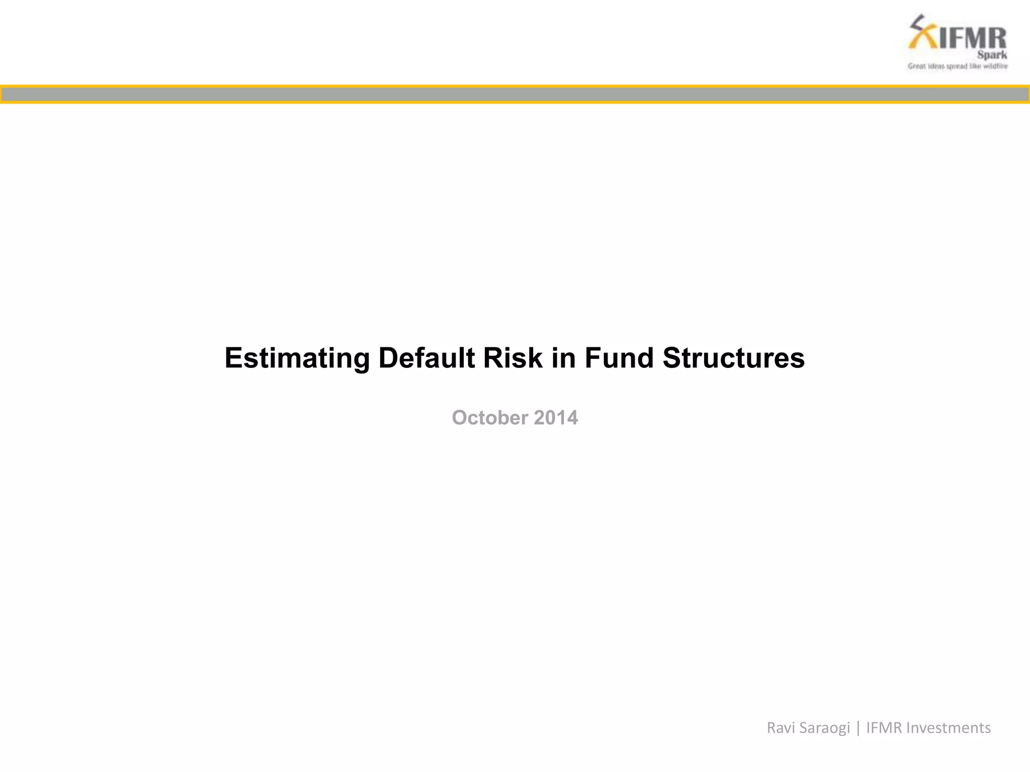
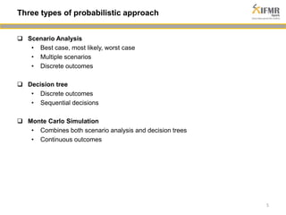
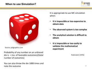
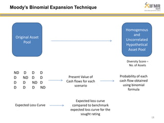
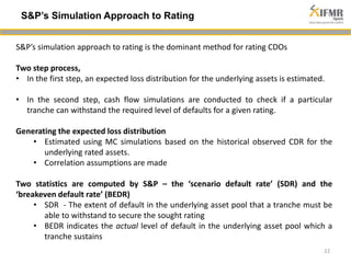
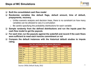
Estimating Default Risk in Fund Structures 
October 2014 
Ravi Saraogi | IFMR Investments
Structure 
2 
 Refresher on MC Simulation 
 Techniques for estimating default risk in Fund structures
• Suppose your commute to work consists of the following: 
– Drive 3 kms on a highway, with 90% probability you will be able to average 20 
KMPH the whole way, but with a 10% probability that a free road will result in 
average speed of 80 KMPH. 
– Come to an intersection with a traffic light that is red for 10 minutes, then green 
for 3 minutes. 
– Travel 1 km, averaging 50 KMMPH with a standard deviation of 10 KMPH. 
– Come to an intersection with a traffic light that is red for 1 minutes, then green for 
30 seconds. 
– Travel 1 more km, averaging 30 KMMPH with a standard deviation of 5 KMPH. 
You want to know how much time to allow for the commute in order to have a 95% 
probability of arriving at work on time. 
3 
How do we solve this?
Non Probabilistic 
• Point estimate – one value as the 
‘best guess’ for the population 
parameter 
• E.g. Sample mean is a point 
estimate for Population mean 
4 
Approach to Uncertainty 
Probabilistic 
• Interval estimate – Range of 
values that is likely to contain the 
population parameter 
• E.g. Sample mean lies within [a.b] 
with 95% confidence (i.e. a 
confidence interval) 
Sample Population 
Statistic Parameter
 Scenario Analysis 
• Best case, most likely, worst case 
• Multiple scenarios 
• Discrete outcomes 
 Decision tree 
• Discrete outcomes 
• Sequential decisions 
 Monte Carlo Simulation 
• Combines both scenario analysis and decision trees 
• Continuous outcomes 
5 
Three types of probabilistic approach
6 
What is Monte Carlo Simulation? 
X 
Y 
Z 
A 
Functional relationship (f) + Random sampling 
(1) Input Distributional 
Assumptions 
(2) (3) 
(4) Output 
distribution 
Uncertainty in 
model inputs 
Uncertainty in 
model outputs
7 
Avoid becoming a Turkey 
Source: http://www.mymoneyblog.com/talebs-thanksgiving- 
turkey.html 
Source: http://nassimtaleb.org/2013/09/turkey-problem/#. 
VFHb1FfGWM8 
Absence of evidence is not evidence of absence
8 
The power of Simulation 
The biggest power of Simulation is to draw a distribution that mimics the actual real life data 
generating process. Once an analyst can get hold of such a distribution, the sky is the limit to 
how she/he wants to dissect the data 
Source: Google Images 
Question: Can we give a range for the minutes its takes to get to office associated 
with the 100% confidence interval?
9 
Origin 
Stanislaw Ulam 
Source: takegame.com Source: en.wikipedia.org 
“…….The question was what are the chances that a Canfield solitaire laid out with 52 
cards will come out successfully? After spending a lot of time trying to estimate 
them by pure combinatorial calculations, I wondered whether a more practical 
method than ‘abstract thinking’ might not be to lay it out say one hundred times and 
simply observe and count the number of successful plays…..” 
-Eckhardt, Roger (1987). Stan Ulam, John von Neumann, and the Monte Carlo method, Los Alamos Science
10 
Analog Computation of Monte Carlo 
Enrico Fermi, Italian physicist 
Source: 
http://en.wikipedia.org/wiki/FERMIAC 
The Monte Carlo trolley, or FERMIAC, was an analog 
computer invented by physicist Enrico Fermi to aid in 
his studies of neutron transport. 
Source: http://en.wikipedia.org/wiki/FERMIAC 
Source: en.wikipedia.org
First Electronic Computation of Monte Carlo 
John Von Neumann, Stanislaw Ulam, and 
Nicholas Metropolis were part of the 
Manhattan project during World War II. 
Source: lanl.gov 
The Manhattan Project 
ENIAC, the first electronic general purpose computer. 
Source: en.wikipedia.org 
Solving the chain reaction in highly enriched uranium was too complex with algebraic equations. 
Hence, simulations were used - plugging many different numbers into the equations and calculating 
the result. Systematically plugging in and trying numbers would have taken too long. So they created 
a new approach -- plugging in randomly chosen numbers into the equations and calculating the 
results.
Impediments 
• Estimating distributions of input variables 
– It is far easier to estimate an expected growth rate of 8% in revenues for the next 
5 years than it is to specify the distribution of expected growth rates – the type of 
distribution, parameters of that distribution. 
• Simulation can be time and resource intensive 
12 
Simulation: Keep in mind 
Benefits 
• Simulation gives a way out when stuck against a complicated intractable 
mathematical dilemma 
• Output is a distribution rather than a point estimate 
– Investment with a higher expected return may have a fat tailed distribution 
Pitfalls 
• Garbage in, garbage out: For simulations to have value, the distributions should be 
based upon analysis and data, rather than guesswork 
• Benefits that decision-makers get by having a fuller picture of the uncertainty may be 
more than offset by misuse of simulation
13 
When to use Simulation? 
It is appropriate to use MC simulation 
when: 
• It is impossible or too expensive to 
obtain data 
• The observed system is too complex 
• The analytical solution is difficult to 
obtain 
• It is impossible or too costly to 
validate the mathematical 
experiment 
Probability of any number on an unbiased 
die is = (no. of favorable outcomes)/(total 
number of outcomes) 
You can also throw the die 1000 times and 
note the outcome 
-Rubinstein (1976) 
Source: psdgraphics.com
• VaR for a single asset 
– Assume normality 
– Mean of Rs 120 lakhs and an annual standard deviation of Rs 10 lakhs 
– With 95% confidence, you can say that the value of this asset will not drop below 
Rs 100 lakhs (two standard deviations below from the mean) or rise above Rs 
140 lakhs (two standard deviations above the mean) over the next year. 
14 
Risk for a single asset 
Source: Google Images
15 
Risk for a portfolio of assets 
• VaR for a portfolio of assets 
o Assume normality 
o Portfolio consists of 10 individual assets with mean value varying from INR 
50 lakhs to INR 950 lakhs 
o Standard deviation varies from INR 5 lakh to INR 100 lakh
16 
Evaluating risk in a Fund Structure 
Bond 1 
Costs 
Interest Received 
Investor Payouts 
Repayments 
Reinvestments 
Bond 2 
Bond 3 
Bond 10 
Structure 
P(d)) 
Investor Return 
P(d)) 
P(d)) 
P(d))
• One of the earliest known methodology introduced in 1996 
• This method creates a hypothetical portfolio of uncorrelated and homogenous assets 
from the original asset pool. 
17 
Moody’s Binomial Expansion Technique 
Statistic Description 
Step 1: 
Diversity Score (DS) 
Reduction of the heterogeneous asset pool into homogeneous and independent 
assets. The higher the concentration of assets in the underlying pool, the lower 
the DS 
Step 2: 
Cash flow computations 
Generating cash flows for combinations of each possible homogenous bonds 
defaulting 
Step 3: 
Tranche cash flows 
Putting the cash flows generated in Step 2 through the tranche waterfall to check 
for losses. In this step, other variables, like interest rates, can also be changed to 
account for different scenarios 
Step 4: 
Determine default probability 
The default probability is determined based on output from Step 3 and after 
taking into consideration the tenure and rating 
Step 5: 
Deriving the loss distribution 
curve 
Based on the different scenarios in Step 3 and the default probabilities 
calculated in Step 4 for each scenario, the loss distribution curve is derived 
Step 6: 
Comparing loss distribution 
The loss distribution in Step 5 is compared to a target loss distribution for a 
tranche to see if the credit enhancement is adequate for the sought rating
18 
Moody’s Binomial Expansion Technique 
Original Asset 
Pool 
Homogenous 
and 
Uncorrelated 
Hypothetical 
Asset Pool 
Diversity Score – 
No. of Assets 
ND D D D 
D ND D D 
D D ND D 
D D D ND 
Present Value of 
Cash flows for each 
scenario 
Probability of each 
cash flow obtained 
using binomial 
formula 
Expected Loss Curve 
Expected loss curve 
compared to benchmark 
expected loss curve for the 
sought rating
• Restrictive assumptions 
• Useful only when the size of holdings and default probability distributions are 
homogenous in the collateral pool. 
• The correlation factor is reduced to zero in the constructed hypothetical portfolio. 
• BET fails the accuracy test when DS is less than the total number of assets in the 
original pool, which will be an almost always case due to the presence of contagion 
effects and correlation in the larger asset pool. 
• Inverse relationship between correlation and DS 
Moody’s had dealt with this issue by upward adjustment of the calculated portfolio default 
rates based on the WAR of the pool . Such an approach is open to criticisms of ad hoc 
adjustments to the model. 
19 
Criticisms
• It is impossible or too expensive to obtain data 
• The observed system is too complex 
• The analytical solution is difficult to obtain 
• It is impossible or too costly to validate the mathematical experiment 
Thus, based on Rubinstein’s four criteria, the use of MC simulations for CDO rating is 
justified. 
20 
Can we use Simulation instead?
21 
S&P’s Simulation Approach to Rating 
*For methodology sanctity, the model assumptions used in both Step 1 and Step 2 should be the same, 
else the SDRs obtained from Step 1 cannot be compared to BEDRs obtained from Step 2 
** Scenario Default Rates *** Break-Even Default Rates
22 
S&P’s Simulation Approach to Rating 
S&P’s simulation approach to rating is the dominant method for rating CDOs 
Two step process, 
• In the first step, an expected loss distribution for the underlying assets is estimated. 
• In the second step, cash flow simulations are conducted to check if a particular 
tranche can withstand the required level of defaults for a given rating. 
Generating the expected loss distribution 
• Estimated using MC simulations based on the historical observed CDR for the 
underlying rated assets. 
• Correlation assumptions are made 
Two statistics are computed by S&P – the ‘scenario default rate’ (SDR) and the 
‘breakeven default rate’ (BEDR) 
• SDR - The extent of default in the underlying asset pool that a tranche must be 
able to withstand to secure the sought rating 
• BEDR indicates the actual level of default in the underlying asset pool which a 
tranche sustains
23 
The Scenario Default Rate 
12% 
10% 
8% 
6% 
4% 
2% 
0% 
SDR (AA) = 37%, 
CDR = 0.51% 
1% 
3% 
5% 
7% 
9% 
11% 
13% 
15% 
17% 
19% 
21% 
23% 
25% 
27% 
29% 
31% 
33% 
35% 
37% 
39% 
41% 
43% 
45% 
47% 
Probability 
Default rates in the underlying portfolio 
SDR (AAA) = 43%, 
CDR=0.15% 
If the expected default rate of a10-year AAA-rated corporate bond is 0.15%, the SDR for the 
tranche (which aspires to be rated AAA) is set equal to the level of default in the CDO’s collateral 
pool that has no greater than 0.15% chance of being exceeded. The logic is ‘‘if the tranche can 
survive defaults up to the SDR then its probability of default is no greater than 0.15%, as would 
be appropriate for an AAA rating’’ (Global Cash Flow and Synthetic CDO Criteria, p.42).
24 
Consolidated Approach 
*Model assumptions are coded in the consolidated model to ensure uniformity of structure across the 
cash flow model and the CDO model.
25 
The difference is the use of historical default rates 
http://www.standardandpoors.com/ratings/articles/en/us/?articleType=HTML&assetID=1245331158575
 Built the consolidated cash flow model 
 Randomize variables like default flags, default amount, time of default, 
prepayments, recovery. 
o Unlike scenario analysis and decision trees, there is no constraint on how many 
variables can be allowed to vary in a simulation 
o Be careful specifying the probability distributions for each variable 
 Sample randomly from the defined distributions and run the inputs past the 
cash flow model to get the payouts 
 For each trial, run the payouts against the waterfall and record if the cash flows 
were sufficient to meet each tranche commitment or not 
 Compare the default instances with the historical default studies to impute 
rating 
26 
Steps of MC Simulations 
Source: CRISIL Default Study, 2012
What is at stake? 
27 
Conversion of low rated underlying pool assets into high rated tranches in the US 
subprime crisis highlights the need for better understanding 
Source: Efraim Benmelech, Jennifer Dlugosz, 2009, The Alchemy of CDO Ratings, NBER 
Working Paper Series 14878
28 
Thank you

Estimating default risk in fund structures

  • 1.
    Estimating Default Riskin Fund Structures October 2014 Ravi Saraogi | IFMR Investments
  • 2.
    Structure 2 Refresher on MC Simulation  Techniques for estimating default risk in Fund structures
  • 3.
    • Suppose yourcommute to work consists of the following: – Drive 3 kms on a highway, with 90% probability you will be able to average 20 KMPH the whole way, but with a 10% probability that a free road will result in average speed of 80 KMPH. – Come to an intersection with a traffic light that is red for 10 minutes, then green for 3 minutes. – Travel 1 km, averaging 50 KMMPH with a standard deviation of 10 KMPH. – Come to an intersection with a traffic light that is red for 1 minutes, then green for 30 seconds. – Travel 1 more km, averaging 30 KMMPH with a standard deviation of 5 KMPH. You want to know how much time to allow for the commute in order to have a 95% probability of arriving at work on time. 3 How do we solve this?
  • 4.
    Non Probabilistic •Point estimate – one value as the ‘best guess’ for the population parameter • E.g. Sample mean is a point estimate for Population mean 4 Approach to Uncertainty Probabilistic • Interval estimate – Range of values that is likely to contain the population parameter • E.g. Sample mean lies within [a.b] with 95% confidence (i.e. a confidence interval) Sample Population Statistic Parameter
  • 5.
     Scenario Analysis • Best case, most likely, worst case • Multiple scenarios • Discrete outcomes  Decision tree • Discrete outcomes • Sequential decisions  Monte Carlo Simulation • Combines both scenario analysis and decision trees • Continuous outcomes 5 Three types of probabilistic approach
  • 6.
    6 What isMonte Carlo Simulation? X Y Z A Functional relationship (f) + Random sampling (1) Input Distributional Assumptions (2) (3) (4) Output distribution Uncertainty in model inputs Uncertainty in model outputs
  • 7.
    7 Avoid becominga Turkey Source: http://www.mymoneyblog.com/talebs-thanksgiving- turkey.html Source: http://nassimtaleb.org/2013/09/turkey-problem/#. VFHb1FfGWM8 Absence of evidence is not evidence of absence
  • 8.
    8 The powerof Simulation The biggest power of Simulation is to draw a distribution that mimics the actual real life data generating process. Once an analyst can get hold of such a distribution, the sky is the limit to how she/he wants to dissect the data Source: Google Images Question: Can we give a range for the minutes its takes to get to office associated with the 100% confidence interval?
  • 9.
    9 Origin StanislawUlam Source: takegame.com Source: en.wikipedia.org “…….The question was what are the chances that a Canfield solitaire laid out with 52 cards will come out successfully? After spending a lot of time trying to estimate them by pure combinatorial calculations, I wondered whether a more practical method than ‘abstract thinking’ might not be to lay it out say one hundred times and simply observe and count the number of successful plays…..” -Eckhardt, Roger (1987). Stan Ulam, John von Neumann, and the Monte Carlo method, Los Alamos Science
  • 10.
    10 Analog Computationof Monte Carlo Enrico Fermi, Italian physicist Source: http://en.wikipedia.org/wiki/FERMIAC The Monte Carlo trolley, or FERMIAC, was an analog computer invented by physicist Enrico Fermi to aid in his studies of neutron transport. Source: http://en.wikipedia.org/wiki/FERMIAC Source: en.wikipedia.org
  • 11.
    First Electronic Computationof Monte Carlo John Von Neumann, Stanislaw Ulam, and Nicholas Metropolis were part of the Manhattan project during World War II. Source: lanl.gov The Manhattan Project ENIAC, the first electronic general purpose computer. Source: en.wikipedia.org Solving the chain reaction in highly enriched uranium was too complex with algebraic equations. Hence, simulations were used - plugging many different numbers into the equations and calculating the result. Systematically plugging in and trying numbers would have taken too long. So they created a new approach -- plugging in randomly chosen numbers into the equations and calculating the results.
  • 12.
    Impediments • Estimatingdistributions of input variables – It is far easier to estimate an expected growth rate of 8% in revenues for the next 5 years than it is to specify the distribution of expected growth rates – the type of distribution, parameters of that distribution. • Simulation can be time and resource intensive 12 Simulation: Keep in mind Benefits • Simulation gives a way out when stuck against a complicated intractable mathematical dilemma • Output is a distribution rather than a point estimate – Investment with a higher expected return may have a fat tailed distribution Pitfalls • Garbage in, garbage out: For simulations to have value, the distributions should be based upon analysis and data, rather than guesswork • Benefits that decision-makers get by having a fuller picture of the uncertainty may be more than offset by misuse of simulation
  • 13.
    13 When touse Simulation? It is appropriate to use MC simulation when: • It is impossible or too expensive to obtain data • The observed system is too complex • The analytical solution is difficult to obtain • It is impossible or too costly to validate the mathematical experiment Probability of any number on an unbiased die is = (no. of favorable outcomes)/(total number of outcomes) You can also throw the die 1000 times and note the outcome -Rubinstein (1976) Source: psdgraphics.com
  • 14.
    • VaR fora single asset – Assume normality – Mean of Rs 120 lakhs and an annual standard deviation of Rs 10 lakhs – With 95% confidence, you can say that the value of this asset will not drop below Rs 100 lakhs (two standard deviations below from the mean) or rise above Rs 140 lakhs (two standard deviations above the mean) over the next year. 14 Risk for a single asset Source: Google Images
  • 15.
    15 Risk fora portfolio of assets • VaR for a portfolio of assets o Assume normality o Portfolio consists of 10 individual assets with mean value varying from INR 50 lakhs to INR 950 lakhs o Standard deviation varies from INR 5 lakh to INR 100 lakh
  • 16.
    16 Evaluating riskin a Fund Structure Bond 1 Costs Interest Received Investor Payouts Repayments Reinvestments Bond 2 Bond 3 Bond 10 Structure P(d)) Investor Return P(d)) P(d)) P(d))
  • 17.
    • One ofthe earliest known methodology introduced in 1996 • This method creates a hypothetical portfolio of uncorrelated and homogenous assets from the original asset pool. 17 Moody’s Binomial Expansion Technique Statistic Description Step 1: Diversity Score (DS) Reduction of the heterogeneous asset pool into homogeneous and independent assets. The higher the concentration of assets in the underlying pool, the lower the DS Step 2: Cash flow computations Generating cash flows for combinations of each possible homogenous bonds defaulting Step 3: Tranche cash flows Putting the cash flows generated in Step 2 through the tranche waterfall to check for losses. In this step, other variables, like interest rates, can also be changed to account for different scenarios Step 4: Determine default probability The default probability is determined based on output from Step 3 and after taking into consideration the tenure and rating Step 5: Deriving the loss distribution curve Based on the different scenarios in Step 3 and the default probabilities calculated in Step 4 for each scenario, the loss distribution curve is derived Step 6: Comparing loss distribution The loss distribution in Step 5 is compared to a target loss distribution for a tranche to see if the credit enhancement is adequate for the sought rating
  • 18.
    18 Moody’s BinomialExpansion Technique Original Asset Pool Homogenous and Uncorrelated Hypothetical Asset Pool Diversity Score – No. of Assets ND D D D D ND D D D D ND D D D D ND Present Value of Cash flows for each scenario Probability of each cash flow obtained using binomial formula Expected Loss Curve Expected loss curve compared to benchmark expected loss curve for the sought rating
  • 19.
    • Restrictive assumptions • Useful only when the size of holdings and default probability distributions are homogenous in the collateral pool. • The correlation factor is reduced to zero in the constructed hypothetical portfolio. • BET fails the accuracy test when DS is less than the total number of assets in the original pool, which will be an almost always case due to the presence of contagion effects and correlation in the larger asset pool. • Inverse relationship between correlation and DS Moody’s had dealt with this issue by upward adjustment of the calculated portfolio default rates based on the WAR of the pool . Such an approach is open to criticisms of ad hoc adjustments to the model. 19 Criticisms
  • 20.
    • It isimpossible or too expensive to obtain data • The observed system is too complex • The analytical solution is difficult to obtain • It is impossible or too costly to validate the mathematical experiment Thus, based on Rubinstein’s four criteria, the use of MC simulations for CDO rating is justified. 20 Can we use Simulation instead?
  • 21.
    21 S&P’s SimulationApproach to Rating *For methodology sanctity, the model assumptions used in both Step 1 and Step 2 should be the same, else the SDRs obtained from Step 1 cannot be compared to BEDRs obtained from Step 2 ** Scenario Default Rates *** Break-Even Default Rates
  • 22.
    22 S&P’s SimulationApproach to Rating S&P’s simulation approach to rating is the dominant method for rating CDOs Two step process, • In the first step, an expected loss distribution for the underlying assets is estimated. • In the second step, cash flow simulations are conducted to check if a particular tranche can withstand the required level of defaults for a given rating. Generating the expected loss distribution • Estimated using MC simulations based on the historical observed CDR for the underlying rated assets. • Correlation assumptions are made Two statistics are computed by S&P – the ‘scenario default rate’ (SDR) and the ‘breakeven default rate’ (BEDR) • SDR - The extent of default in the underlying asset pool that a tranche must be able to withstand to secure the sought rating • BEDR indicates the actual level of default in the underlying asset pool which a tranche sustains
  • 23.
    23 The ScenarioDefault Rate 12% 10% 8% 6% 4% 2% 0% SDR (AA) = 37%, CDR = 0.51% 1% 3% 5% 7% 9% 11% 13% 15% 17% 19% 21% 23% 25% 27% 29% 31% 33% 35% 37% 39% 41% 43% 45% 47% Probability Default rates in the underlying portfolio SDR (AAA) = 43%, CDR=0.15% If the expected default rate of a10-year AAA-rated corporate bond is 0.15%, the SDR for the tranche (which aspires to be rated AAA) is set equal to the level of default in the CDO’s collateral pool that has no greater than 0.15% chance of being exceeded. The logic is ‘‘if the tranche can survive defaults up to the SDR then its probability of default is no greater than 0.15%, as would be appropriate for an AAA rating’’ (Global Cash Flow and Synthetic CDO Criteria, p.42).
  • 24.
    24 Consolidated Approach *Model assumptions are coded in the consolidated model to ensure uniformity of structure across the cash flow model and the CDO model.
  • 25.
    25 The differenceis the use of historical default rates http://www.standardandpoors.com/ratings/articles/en/us/?articleType=HTML&assetID=1245331158575
  • 26.
     Built theconsolidated cash flow model  Randomize variables like default flags, default amount, time of default, prepayments, recovery. o Unlike scenario analysis and decision trees, there is no constraint on how many variables can be allowed to vary in a simulation o Be careful specifying the probability distributions for each variable  Sample randomly from the defined distributions and run the inputs past the cash flow model to get the payouts  For each trial, run the payouts against the waterfall and record if the cash flows were sufficient to meet each tranche commitment or not  Compare the default instances with the historical default studies to impute rating 26 Steps of MC Simulations Source: CRISIL Default Study, 2012
  • 27.
    What is atstake? 27 Conversion of low rated underlying pool assets into high rated tranches in the US subprime crisis highlights the need for better understanding Source: Efraim Benmelech, Jennifer Dlugosz, 2009, The Alchemy of CDO Ratings, NBER Working Paper Series 14878
  • 28.