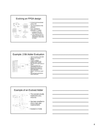
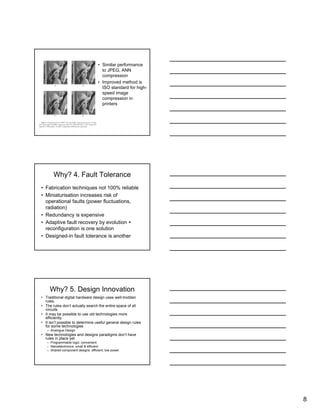
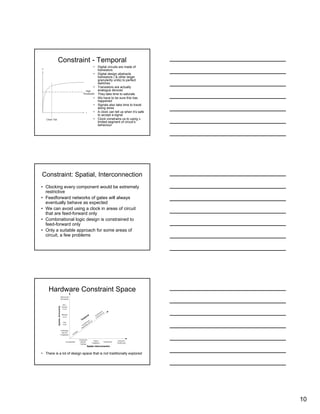
1. 1
Hardware Evolution
4C57/GI06 Evolutionary Systems
Tim Gordon
What is Hardware Evolution?
• The application of evolutionary techniques to
hardware design and synthesis
• It is NOT just hardware implementation of EA
• Also called: Evolvable Hardware
Evolutionary Electronics
Where is Hardware Evolution?
• Many learning algorithms
are inspired by nature
- GA/GP
- ANNs
- Immune Systems
- Ant Colony Optimisation
• Nature also inspires
hardware designers
- Spiking ANNs
- Fault tolerance
- Design Optimisation
Biology
Computer
Science
Electronic Engineering
Evolvable
Hardware
Bio-
inspired
Hardware
Bio-
inspired
Software
Systems
Engineering

2. 2
How is Evolution Applied?
• Digital Hardware
Design = Logic
Synthesis + Mapping
• Both processes
involve optimisation
steps
• Most interest in
evolving design +
mapping at once
Evolutionary
Design
Evolvable
Hardware
Evolutionary Logic
Design
Evolutionary
Map, Place,
Route
Technology Map,
Place, Route
Logic
Synthesis
Hardware
Synthesis
HE Example: Reconfigurable
Hardware
• There are chips where the behaviour of all the
components can be programmed
• There are chips where the interconnections
between the components can also be
programmed
• The program that places a circuit design on the
chip is called a bitstream.
• Once written, the chip will stay configured with
the design until bitstream is rewritten
• One type of reconfigurable chip is a Field
Programmable Gate Array
Field Programmable Gate Array
• FPGAs are 2D arrays of cells
• Cells are called Configurable Logic Blocks
• CLBs connected together with wires to/from nearest neighbours
• Each cell contains logic, and switches to select inputs & outputs
Out 1F LUT
Out 2G LUT
Inp 1
Inp 2
Inp 3
Inp 4
Cell Cell
Cell Cell CellCell
Cell Cell CellCell
Cell Cell CellCell
Cell Cell

3. 3
CLB Example
• The logic within CLBs is
usually several lookup tables
(LUTs) + other stuff
• This example has 2x 4 Input
LUTs, labelled F and G
• A 4-input LUT can implement
any logical function of 4 inputs
• The logical function of LUT is
defined by the truthtable output
bits
• A LUT can be programmed by
setting the corresponding bits
in the bitstream
G
LUT
0
0
0
0
0
0
0
0
0
0
0
0
1
1
1
1
0
1
0
1
0
1
0
1
0
1
0
1
0
1
0
1
0
0
1
1
0
0
1
1
0
0
1
1
0
0
1
1
0
0
0
0
1
1
1
1
0
0
0
0
1
1
1
1
0
0
0
0
0
0
0
0
1
1
1
1
1
1
1
1
Inp1 Inp2 Inp3 Inp4 Output
F
LUT
Output =
AND(Inp1,Inp2)
F LUT
Truthtable:
0
0
0
0
0
0
0
0
0
0
0
0
1
1
1
1
.
.
.
.
.
.
.
.
.
.
.
.
.
.
Bitstream
fragment:
Inputs Example
• Inputs can be selected from
the LUT outputs of 4
neighbouring cells
• An input is selected by a
special configuration
multiplexer
• 8 possible inputs = 3 bits per
MUX
• Inputs programmed by setting
corresponding configuration
bits in the bitstream
Input 1
Input4
Input2
Input 3
F
LUT
G
LUT
F
North
G
North
F
East
G
East
G
South
F
South
F
West
G
West
F
North
G
North
F
East
G
East
G
South
F
South
F
West
G
West
F
North
G
North
F
East
G
East
G
South
F
South
F
West
G
West
F
North
G
North
F
East
G
East
G
South
F
South
F
West
G
West
010
011
100
000
000010011100 …….…….
Input
Configuration
Bits:
Bitstream Fragment:
Bitstream Example
• Bitstream consists of a concatenation of all
configuration bits
• Example shows bitstream fragment for 1 CLB
000010011100 …….……. 0000000000001111
Bitstream fragment:
0101010101010101
CLB Input
Bits
F LUT
Bits
G LUT
Bits

4. 4
Evolving an FPGA design
• A circuit can be evolved
using a GA
• The chromosome is the
bitstream
• Each individual is
evaluated in 2 steps:
1: Configure FPGA with
bitstream/chromosome
2. Test configured FPGA by
applying all possible input
combinations, using output
for fitness
0 10110 101 1
1 10010 100 1
1 10111 010 0
1 10100 110 0
1 11010 010 1
1 10010 010 0
1 10100 110 0
Fitness
30
14
14
28
18
0 10110 101 1
1 10111 100 1
1 11010 010 1
1 11010 010 1
1 10111 100 1
1 111 11 010 1
1 010 10 100 1
1 110 01 000 1
1 110 10 100 0
2. Evaluate Circuit
3. Select Breeding Pairs
1. Create New Population
4. Cross Over
5. Mutate6. Insert Into New Population
Iterate until
stopping conditions
are met
Example: 2 Bit Adder Evaluation
• Task is to evolve a 2 Bit adder
• Adds 2x 2 bit numbers
together
• 4 inputs, 2 outputs
• Create a truthtable of all
possible inputs / outputs
• Pick input and output points on
FPGA
• Pass all possible input
combinations one at a time
• Measure total number of
output bits correct for each
input combination
• Fitness = sum(correct output
bits)
• Set of all input combinations
called training set
0
0
0
0
0
0
0
0
1
1
1
1
1
1
1
1
0
0
0
0
1
1
1
1
0
0
0
0
1
1
1
1
0
0
1
1
0
0
1
1
0
0
1
1
0
0
1
1
0
1
0
1
0
1
0
1
0
1
0
1
0
1
0
1
0
0
1
1
0
1
1
0
1
1
0
0
1
0
0
1
A B
0
1
0
1
1
0
1
0
0
1
0
1
1
0
1
1
Sum1Sum0
FPGAA1
B0
Sum0
Sum1
B1
A0
Example of an Evolved Adder
B0
C In
A0
B1
A1
S1
C Out
S0
• This example actually
implements carry
in/out too
• Has been simplified to
show a logic gate
implementation
• Evolved in 2 CLBs

5. 5
Is it practical?
• For most real-world hardware problems
human designers outperform evolution
• Solving the problems that limit HE is an
active area of research
• This research discussed later
• BUT
– Hardware evolution does have niches
Why? 1. Lowers Costs
• Automatic design = low cost hardware
• Low design cost makes low volumes more acceptable
• HE + field-reconfigurable hardware allows one-off
designs (Kajitani et al. 1999)
• Integrated circuit manufacture is not perfect
• Variations in manufacture result in substandard
performance
• Evolution can tune circuits to take account of variations
• This improve yields (Mukarawa et al. 1998)
One-off design e.g.: Myoelectric arm controller
• Traditionally user must learn to
control arm
• Task is to learn to control
actuators from nerve signals
• Inputs are Fourier transformed
nerve data (training set) from
user
• Outputs are control signals for
actuator
• Successfully evolved circuits to
control arm for individual users
• Circuit automatically
implemented on reconfigurable
chip
• Hardware solution is small &
light

6. 6
Why? (2) Poorly Specified
Problems
• Can’t easily design solution to these problems
• When applied to ANN-type problems
– Faster operation and design
– Easier to analyse
• HE tends to evolve feed-forward networks of
logic gates for such problems: avoids some
problems
e.g. classifiers (Higuchi, Iwata et al. 1996)
image filters (Sekanina 2003)
Myoelectric Arm Revisited
• Evolved 1 control circuit for each actuator
• 200 training patterns of each movement
• 800 training patters of no movement
• Slightly better than 64 node backprop ANN
- 85% rather than 80%
• Much faster learning (80 ms rather than 3
hours on 200MHz PC)
Why? 3. Adaptive Systems
• HE + reconfigurable hardware = real-time
adaptation
• Can adapt autonomously to changes in
environment
• Useful when real-time manual control not
possible
– E.g. spacecraft systems (sensor processing)
• Non-critical systems are more suitable
– E.g. data compression systems
– plant power management
– ATM cell scheduling

7. 7
Image Compression Example
• Pixels in an image tend to tightly correlate
with their neighbours
• Pixel value can usually be predicted from
neighbours
• Compressed image = prediction function +
error at each pixel (lossless)
JPEG Compression
• Prediction function
based on surrounding
pixels
• Image is broken into
blocks
• For each block a
prediction function is
selected
Hardware Evolution Compression
• Prediction function is evolved on reconfigurable
hardware
• Evolve a circuit for each 16x16 block:
– Input: image data, 4 pixels x 8b = 32 inputs, all 256 training
cases
– Output: predicted pixel
– Fitness: compare predicted with raw, sum(error for 16x16 block)
– Aim is to minimise error
• Each circuit = compression function for a 16x16 block
• Total compressed image size = sum(chromosome bits
for each circuit + error bits for each pixel)

8. 8
• Similar performance
to JPEG, ANN
compression
• Improved method is
ISO standard for high-
speed image
compression in
printers
Why? 4. Fault Tolerance
• Fabrication techniques not 100% reliable
• Miniaturisation increases risk of
operational faults (power fluctuations,
radiation)
• Redundancy is expensive
• Adaptive fault recovery by evolution +
reconfiguration is one solution
• Designed-in fault tolerance is another
Why? 5. Design Innovation
• Traditional digital hardware design uses well-trodden
rules.
• The rules don’t actually search the entire space of all
circuits
• It may be possible to use old technologies more
efficiently
• It isn’t possible to determine useful general design rules
for some technologies
– Analogue Design
• New technologies and designs paradigms don’t have
rules in place yet
– Programmable logic: convenient
– Nanoelectronics: small & efficient
– Shared component designs: efficient, low power

9. 9
Can Evolution Really Innovate With
Standard Technologies?
• Traditional design works from the top
down
• Design rules limit interactions between
components to a tractable level
• Evolution tinkers with designs from the
bottom up
• Hence it might be searching non-
traditional areas of space
• More on whether it actually can later
Classifying HE – Level of
Constraint
• Both software and hardware design rely on
abstraction
• Abstraction simplifies large problems
• When we use a design abstraction we need to
make sure the hardware actually behaves
according to the abstraction
• i.e. we need to constrain the hardware to
particular behaviours
• Constraints are spatial (granularity), spatial
(interconnection) or temporal
Constraint – Spatial, Granularity
• All traditional design methodologies use encapsulation
• Designers like to describe their problems with large well-understood
units
• Digital designers encapsulate collections of transistors into gates,
gates into adders, registers etc.
• Analogue designers encapsulate collections of components into
amplifiers, filters etc.
• This limits the interactions within the circuits
• Interactions can only take place between the interfaces of the
chosen units
– i.e. the internals of one unit can’t interact with another
• Hence it actually constrains the types of circuit we explore

10. 10
Constraint - Temporal
• Digital circuits are made of
transistors
• Digital design abstracts
transistors ( & other larger
granularity units) to perfect
switches
• Transistors are actually
analogue devices
• They take time to saturate
• We have to be sure this has
happened
• Signals also take time to travel
along wires
• A clock can tell us when it’s safe
to accept a signal
• Clock constrains us to using v.
limited segment of circuit’s
behaviour
Constraint: Spatial, Interconnection
• Clocking every component would be extremely
restrictive
• Feedforward networks of gates will always
eventually behave as expected
• We can avoid using a clock in areas of circuit
that are feed-forward only
• Combinational logic design is constrained to
feed-forward only
• Only a suitable approach for some areas of
circuit, a few problems
Hardware Constraint Space
Tem
poral
Asynchronous
Synchronous
Analogue
(Handshake-driven)
(Clock-driven)
Spatial, Interconnection
Spatial,Granularity
Unconstrained
Architecture
Specific
Topology
Technology
Specific
Components
Nearest
Neighbours
Feedforward
Restricted
Feedforward
Gate
Level
RTL /
Function
Level
Behavioural
Descriptions
Bistream
Level
• There is a lot of design space that is not traditionally explored

11. 11
Classifying HE – Evaluation
Strategy
• Early HE used evaluated circuits in
simulation: Extrinsic HE
• Simulating logical abstractions is efficient
• Simulating low-constraint HE is
computationally expensive
• Simulating low-constraint is difficult
Evaluation Strategy (2)
• Evaluating with a programmable logic device is called Intrinsic HE
• Disadvantages are:
– Limited reconfigurability
– Speed of reconfiguration
– Destructibility
– Limited topology and granularity
– Limited observability
• The most versatile programmable logic device is the FPGA
• Commercial FPAAs also available but to date limited by one or more
of the above
• Only a few research platforms actually designed for evolution
Innovation Research – Traditional
vs. Evolutionary Search
• Traditional design decomposes from the top
down into known sub-problems
• Applies constraints to ensure design behaves
like known sub-problems
• Evolution works from the bottom up
• Evolution uses fitness to guide performance
• Not directed by prior knowledge
• Oblivious to complexities of the interactions
within the circuit

12. 12
Relaxing Constraints
• There may be innovative circuits in space
beyond traditional design
• But can evolution actually manipulate circuit
dynamics / structure when traditional constraints
are relaxed?
• Gates have delays measured in ns
• Inputs and outputs of interest are often much
slower
• Traditionally temporal constraints are used to
achieve this
• Can evolution manipulate fast components into
a configuration that behaves more slowly?
Evolving an Oscillator
• Evolved a network of high-speed gates at to behave as a
low frequency oscillator (Thompson, Harvey et al. 1996)
• Few constraints: none on connectivity or temporal, gate
level granularity
• Aim: Oscillate every 0.5ms, using gates with 1-5ns
delays
• Fitness =
1. Measure time b/w each oscillation
2. Calculate difference b/w oscillation time & 0.5ms
3. Sum error over 10ms (simulated) evaluation time
Chromosome Structure
• Defines network of gates
• Array of 100 segments as
shown in table
• Each segment describes a
component + connections
• Node function: gate type
• Length: how many segments
to count
• Direction: count
forwards/backwards
• Addressing mode: count from
current segment / start of array

13. 13
Best Circuit Evolved
Oscillator Performance
• Evolution really can find potentially useful circuits (low-
speed behaviour) with no design constraints (only
high-speed gates)
Relaxing Constraints – Intrinsic
• Can this be achieved with real hardware?
• Evolved circuit to discriminate between two
frequencies
• To discriminate b/w frequencies circuit must
measure oscillations over a (relatively) long time
• Evolved entire bitstream for a 10x10 cell area of
FPGA
• Only real, fast-saturating FPGA gates available

14. 14
Thompson’s Frequency
Discriminator
• 1 input, 1 output
• No clock signal
available
• Fitness:
– Maximise difference
b/w output voltage
when 1kHz or 10kHz
signals applied
Can Evolution Find Innovative
Circuits?
• Circuits that could not be found using
traditional design abstractions are
innovative
• Solution has high performance
• Uses less gates that traditional designs
• Analysis shows internal non-digital
behaviour
∴ Innovative
Problems with innovative circuits
• Important to understand how a circuit
works
• Some behaviour defies analysis
• Not portable
– Fails on other FPGAs
– Fails when temperature changed
• These problems have to be tackled before
evolved innovative circuits are useful

15. 15
Innovation in Digital Design Space
• Are there innovative circuits that don’t
break the digital design constraints?
• Expt. repeated with clock as additional
input
• Solutions used clock, simulated perfectly
on logic simulator
• Analysis revealed solution could not be
discovered by traditional top-down design
Innovation – New Technologies
• Traditional design maps to AND, OR gates
• FPGAs use XOR, LUTs and MUXs
• Can evolution make better use of these
gates?
• Evolved 3 bit multipliers
– i.e. multiplies 2x 3bit numbers together
Conventional 3 Bit Multiplier
26 gates

16. 16
Evolved 3 bit multiplier
• Fewer gates than traditional design
• Makes much greater use of MUX than traditional design
Innovation – Complex
Technologies
• Traditional analogue design is difficult as it has few rules
– good potential target for HE
• Mutating a digital circuit often causes a big change in
fitness
• Mutating an analogue circuit usually only causes a small
change in fitness
∴ Usually more evolvable than digital
• BUT
– FPAAs are small, restricted topology
– Simulation is computationally expensive
– Simulator has to be very good, e.g. no infinite currents, voltages
• Huge range of circuits evolved, e.g. filters, amplifiers,
computational circuits (i.e. sqrt, log etc)
HE Research - Generalisation
• Evolution is an inductive learner
• Inductive learners infer hypotheses from
observed training examples
• Impossible to train using all possible
combinations of input signals for big problems
• Generalisation vital if HE is to rival traditional
design
• Generalisation to unseen operating conditions
must also be considered
– i.e. portability

17. 17
Approaches to Generalisation
• Hope for the best
• Constrain representation to circuits that
generalise well
• Reward circuits that generalise well
through fitness function
– Evolution must infer the structure along with
the primary task
– More opportunity for innovation
Generalisation to Unseen Inputs
• For some problems feedforward HE outperforms
backprop ANNs on pattern recognition (e.g.
Myoelectric arm)
• Square root function generalises well too
• So hoping for the best can work
BUT
• Arithmetic circuits don’t generalise well
• Applying random subsets of training cases to
reward general circuits doesn’t work
• Why?
Input Generalisation Explained
• Arithmetic functions: all input cases and all bits
contain some unique information
• They all contribute equally to fitness
• Square root: low order bits contribute less to
fitness, can be ignored to some extent
• Pattern recognition: redundant data within input
set
• Redundancy is the key
• Most real-world problems likely to have
redundancy, but it’s a big difficulty

18. 18
Generalisation to Unseen
Environments
• Circuits are expected to function under a range
of conditions:
– Temperature
– Power fluctuations
– Fabrication variations
– Electronic surroundings
– Output load
• Portability a particular problem for unconstrained
HE, intrinsic or extrinsic
Unseen Environments –
Constraining Representation
• Digital design imposes timing constraints
to ensure digital operation
• VLSI foundries test process + set timing,
environmental constraints accordingly
• Exhaustive testing not possible for HE
• Restricting circuit structure to traditional
constraints solves problem
BUT at the expense of innovation
Environmental Generalisation –
Biasing Fitness
• One solution – define an “Operational Envelope” of operating
conditions & evaluate population at different points within it
– non-portable solutions are automatically penalised
• Thompson’s tone discriminator re-evolved using “Operational
Envelope” approach
• Each evaluation carried out on 1 of 5 FPGAs chosen at random:
– Held at different temperatures
– Different power supplies
– Made in different factories
• Evolved solutions were
– Robust across whole temperature range of envelope
– Portable to unseen FPGAs
– Portable to unseen power supplies
∴ Introducing bias towards generalisation can work well

19. 19
Generalisation – Simulation Issues
• Circuit simulation is important - allows analysis
• Logic simulators don’t model all the processes
unconstrained evolution might make use of
• Might not simulate on low-abstraction simulator
too!
– might make use of fabrication, power supply
variations etc.
– these are difficult to replicate in a simulator
• Extrinsic solutions might not work in real life
– low-abstraction simulators often allow infinite currents
voltages
– Evolution often makes use of these
Generalisation – Mixtrinsic
Evolution
• Can do something similar to the operational
envelope:
– During evolution use intrinsic and extrinsic evaluation
– Evaluate circuits at random on either platform
– Non-portable solutions are automatically penalised
– This is called mixtrinsic evaluation
• Could do reverse: reward circuits that are not
portable between intrinsic and extrinsic
– Might promote innovative solutions
Fault Tolerance
• Operation in the presence of faults is
another environmental condition
• Introducing faults during evaluation
improves fault tolerance: just like
Operational Envelope
• EA search bias can cause inherent fault
tolerance to certain conditions
• How?

20. 20
Representational Fault Tolerance
• EAs optimise the population not individual
• Population likely to contain many mutants of
good circuit
• EA is drawn to area where best + mutants are all
high fitness
• If representation is chosen so mutation has
same effect as common fault
– Circuit is identical to mutant
– Mutant still has high fitness because of above
Representational FT: Example
• Hardware often implemented as a finite state machine
• State transitions for FSM can be encoded in RAM
• We could evolve hardware by evolving the RAM bits
• Single Stuck At faults are a common operational fault
• SSA fault would have the same effect on the FSM as a mutation
Output Logic
1 0 0
SSA Fault
000 0 1 0
001 1 0 0
010 0 1 1
011 0 0 1
100 0 0 0
Current
State
Next
State
0
Output Logic
1 0 0
000 0 1 0
001 1 0 0
010 0 1
011 0 0 1
100 0 0 0
Current
State
Next
State
Historical Fault Tolerance
• Introduce fault that breaks best solution (Layzell
and Thompson 2000)
• Some of population usually robust to fault
• EA theory says population should have
converged. What’s going on?
• Earlier best solutions were inherently different
designs
• Crossover often combines these with new best
• Current best is descendent of both designs
• Info about old best retained in population
• Crossover vital to this phenomenon

21. 21
Populational Fault Tolerance
• Population diversity can also allow fault
tolerance
• Shown by evolving population of
oscillators with no shared evolutionary
history (no crossover)
• Faults in one individual did not affect
whole population
• Nicheing might be able to combine PFT &
HFT
HE Research - Evolvability
• Evolvability covers improving:
– Solution quality
– Search performance
– Scalability
• Representation is crucial
• Search space size not as important as order of
search
• Changes in circuit geometry, I/O positioning
often affect performance greatly.
Function Level Evolution
• Aims to improve performance by reducing
search space
• Use domain knowledge to select high-level
building blocks, e.g. add, sub, sin
• Disadvantages:
– Requires designer with domain knowledge
– Not hierachical modularity
– An abstraction that imposes constraint
– Traditional building blocks might not be evolvable

22. 22
Neutral Networks
• EAs converge to suboptimal solutions on large search
spaces
• Traditional thinking says evolution stops when population
converges
• Not necessarily true
• NNs are networks of genotypes with identical fitness
• Genetic drift along NNs allows escape from local optima
• ∴ Evolution continues after genetic convergence
• Many circuit representations have a good deal of
neutrality
• Improves fitness for many HE problems
Incremental Learning
• Break down problem into sub-problems
• Learn solution to 1st sub-problem
• Learn solution to 1st + 2nd sub-problem
• Learn solution to 1st + 2nd + 3rd sub-problem
• Can be automated
• Requires some form of sensible problem
decomposition
– Requires some domain knowledge
Dynamic Representations
• Variable length representation proposed to reduce
search space
• Short representation = small search space
• Start with short representation – reduces initial search
space
• Several researchers have taken similar approach
– Each gene mapped directly to a Boolean function (product term)
– Genes ORed in final solution
– Genes added/removed either by evolutionary operators or
another heuristic
• Improved performance for some pattern recognition
problems reported