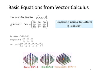
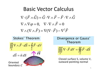
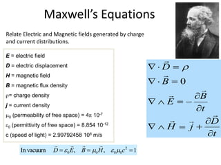
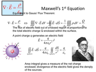
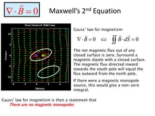
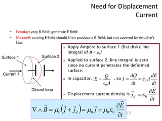
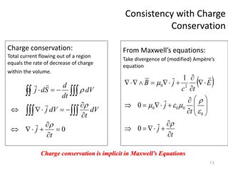
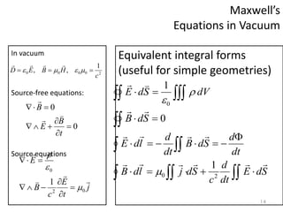
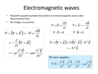
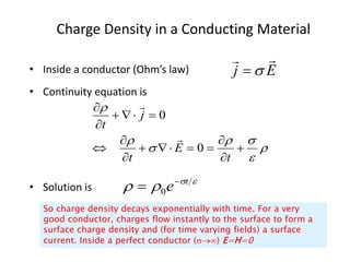
The document discusses Maxwell's equations and electromagnetism, providing an overview of Maxwell's equations which describe the relationship between electric and magnetic fields, motion of charged particles in electromagnetic fields, electromagnetic wave propagation, and basic vector calculus equations. It also lists several textbooks for further reading on classical electromagnetism and provides the source-free and source Maxwell's equations in vacuum.

1. Electromagnetism

2. Contents
• Review of Maxwell’s equations and Lorentz Force Law
• Motion of a charged particle under constant Electromagnetic fields
• Relativistic transformations of fields
• Electromagnetic energy conservation
• Electromagnetic waves
– Waves in vacuo
– Waves in conducting medium
• Waves in a uniform conducting guide
– Simple example TE01 mode
– Propagation constant, cut-off frequency
– Group velocity, phase velocity
– Illustrations
2

3. Reading
• J.D. Jackson: Classical Electrodynamics
• H.D. Young and R.A. Freedman: University Physics (with
Modern Physics)
• P.C. Clemmow: Electromagnetic Theory
• Feynmann Lectures on Physics
• W.K.H. Panofsky and M.N. Phillips: Classical Electricity
and Magnetism
• G.L. Pollack and D.R. Stump: Electromagnetism
3

4. Basic Equations from Vector Calculus
 






































y
F
x
F
x
F
z
F
z
F
y
F
F
z
F
y
F
x
F
F
F
F
F
F
1
2
3
1
2
3
3
2
1
3
2
1
,
,
:
curl
:
divergence
,
,
,
vector
a
For



 
















z
φ
y
φ
x
φ
φ
x,y,z,t
φ
,
,
:
gradient
,
function
scalar
a
For
4
Gradient is normal to surfaces
=constant

5. Basic Vector Calculus
F
F
F
F
G
F
F
G
G
F










2
)
(
)
(
0
,
0
)
(































5
  




S C
r
d
F
S
d
F




dS
n
S
d



Oriented
boundary C
n

Stokes’ Theorem Divergence or Gauss’
Theorem

 



S
V
S
d
F
dV
F



Closed surface S, volume V,
outward pointing normal

6. What is Electromagnetism?
• The study of Maxwell’s equations, devised in 1863 to represent
the relationships between electric and magnetic fields in the
presence of electric charges and currents, whether steady or
rapidly fluctuating, in a vacuum or in matter.
• The equations represent one of the most elegant and concise
way to describe the fundamentals of electricity and magnetism.
They pull together in a consistent way earlier results known from
the work of Gauss, Faraday, Ampère, Biot, Savart and others.
• Remarkably, Maxwell’s equations are perfectly consistent with
the transformations of special relativity.

7. Maxwell’s Equations
Relate Electric and Magnetic fields generated by charge
and current distributions.
1
,
,
In vacuum 2
0
0
0
0 

 c
H
B
E
D 







t
D
j
H
t
B
E
B
D

























0

E = electric field
D = electric displacement
H = magnetic field
B = magnetic flux density
= charge density
j = current density
0 (permeability of free space) = 4 10-7
0 (permittivity of free space) = 8.854 10-12
c (speed of light) = 2.99792458 108 m/s

8. Maxwell’s 1st Equation
0
0
0
1




 Q
dV
S
d
E
dV
E
E
V
S
V









 






0
2
0
3
0
4
4



q
r
dS
q
S
d
E
r
r
q
E
sphere
sphere










0




 E

8
Equivalent to Gauss’ Flux Theorem:
The flux of electric field out of a closed region is proportional to
the total electric charge Q enclosed within the surface.
A point charge q generates an electric field
Area integral gives a measure of the net charge
enclosed; divergence of the electric field gives the density
of the sources.

9. Gauss’ law for magnetism:
The net magnetic flux out of any
closed surface is zero. Surround a
magnetic dipole with a closed surface.
The magnetic flux directed inward
towards the south pole will equal the
flux outward from the north pole.
If there were a magnetic monopole
source, this would give a non-zero
integral.
Maxwell’s 2nd Equation
0


 B

 




 0
0 S
d
B
B



Gauss’ law for magnetism is then a statement that
There are no magnetic monopoles

10. Equivalent to Faraday’s Law of Induction:
(for a fixed circuit C)
The electromotive force round a
circuit is proportional to the
rate of change of flux of magnetic
field, through the circuit.
Maxwell’s 3rd Equation
t
B
E








dt
d
S
d
B
dt
d
l
d
E
S
d
t
B
S
d
E
C S
S
S
















 









 
 l
d
E



 

 S
d
B


N S
Faraday’s Law is the basis for electric
generators. It also forms the basis for
inductors and transformers.

11. Maxwell’s 4th Equation
j
B


0




t
E
c
j
B









2
0
1

I
S
d
j
S
d
B
l
d
B
C S S
   






 0
0 







Originates from Ampère’s (Circuital) Law :
Satisfied by the field for a steady line current (Biot-Savart Law,
1820):
r
I
B
r
r
l
d
I
B





2
4
0
3
0


 
current
line
straight
a
For



Ampère
Biot

12. Need for Displacement
Current
• Faraday: vary B-field, generate E-field
• Maxwell: varying E-field should then produce a B-field, but not covered by Ampère’s
Law.
12
Surface 1 Surface 2
Closed loop
Current I
 Apply Ampère to surface 1 (flat disk): line
integral of B = 0I
 Applied to surface 2, line integral is zero
since no current penetrates the deformed
surface.
 In capacitor, , so
 Displacement current density is
t
E
jd





0

dt
dE
A
dt
dQ
I 0



A
ε
Q
E
0

  t
E
j
j
j
B d













0
0
0
0 




13. Consistency with Charge
Conservation
0

















 


t
j
dV
t
dV
j
dV
dt
d
S
d
j







Charge conservation:
Total current flowing out of a region
equals the rate of decrease of charge
within the volume.
13
From Maxwell’s equations:
Take divergence of (modified) Ampère’s
equation
 
t
j
t
j
E
t
c
j
B













































0
0
1
0
0
0
0
2
0
Charge conservation is implicit in Maxwell’s Equations

14. Maxwell’s
Equations in Vacuum
2
0
0
0
0
1
,
,
c
H
B
E
D 

 







In vacuum
Source-free equations:
Source equations
14
Equivalent integral forms
(useful for simple geometries)
0
0









t
B
E
B



j
t
E
c
B
E




0
2
0
1


















 
















S
d
E
dt
d
c
S
d
j
l
d
B
dt
d
S
d
B
dt
d
l
d
E
S
d
B
dV
S
d
E














2
0
0
1
0
1




15. Example: Calculate E from B






0
0
0
0
sin
r
r
r
r
t
B
Bz


 


 dS
B
dt
d
l
d
E



t
r
B
E
t
B
r
t
B
r
dt
d
rE
r
r










cos
2
1
cos
sin
2
0
0
2
0
2
0








t
r
B
r
E
t
B
r
t
B
r
dt
d
rE
r
r










cos
2
cos
sin
2
0
2
0
0
2
0
0
2
0
0








Also from
t
B
E








dt
E
c
j
B


 



 2
0
1
 then gives current density necessary
to sustain the fields
r
z

16. Lorentz Force Law
• Supplement to Maxwell’s equations, gives force on a charged particle
moving in an electromagnetic field:
• For continuous distributions, have a force density
• Relativistic equation of motion
– 4-vector form:
– 3-vector component:
 
B
v
E
q
f





















 


dt
p
d
dt
dE
c
f
c
f
v
d
dP
F




,
1
, 


16
B
j
E
fd






 
   
B
v
E
q
f
v
m
dt
d 









0

17. Motion of charged particles in constant
magnetic fields
       
B
v
q
v
m
dt
d
B
v
E
q
f
v
m
dt
d 













 
 0
0
17
1. Dot product with v:
 
     
constant
is
constant
is
0
So
1
But
0
2
2
2
0
v
dt
d
dt
d
v
dt
d
v
c
v
γ
B
v
v
m
q
v
dt
d
v






























No acceleration
with a magnetic
field
 
  constant
,
0
0
//
0









v
v
B
dt
d
B
v
B
m
q
v
dt
d
B








2. Dot product with B:

18. Motion in constant magnetic field
 






0
0
0
2
0
frequency
angular
at
radius
with
motion
circular
m
m
m
qB
v
ω
qB
v
m
ρ
B
v
m
q
v
B
v
m
q
dt
v
d
















Constant magnetic field
gives uniform spiral about B
with constant energy.
rigidity
Magnetic
0
q
p
q
v
m
B 




19. Motion in constant Electric Field
Solution of   E
m
q
v
dt
d 

0


c
m
qE
t
m
qE
0
2
0
for
2
1


19
Constant E-field gives uniform acceleration in straight line
      E
q
v
m
dt
d
B
v
E
q
f
v
m
dt
d 











 
 0
0
2
0
2
2
0
1
1 



















 t
m
qE
c
v
t
m
qE
v 



is




















 1
1
2
0
2
0
c
m
qEt
qE
c
m
x
v
dt
dx


qEx
Energy gain is

20. Potentials
• Magnetic vector potential:
• Electric scalar potential:
• Lorentz Gauge:
A
B
A
B











 that
such
0


 



 A
A
f(t)


,
20
0
1
2






A
t
c


 
t
A
E
t
A
E
t
A
E
t
A
A
t
t
B
E























































 so
,
with
0
Use freedom to set

21. Electromagnetic 4-Vectors
21
Α
,
1
,
1
0
1
4
2


























A
c
t
c
A
t
c




Lorentz
Gauge
4-gradient
4
4-potential A
Current
4-vector 







0
0
0 where
)
,
(
)
,
( 





j
c
v
c
V
J
v
j




Continuity
equation   0
,
,
1
4 


















 j
t
j
c
t
c
J

 

Charge-current
transformations
  










 2
,
c
j
v
v
j
j x
x
x 





22. Example: Electromagnetic Field of a Single Particle
• Charged particle moving along x-axis of Frame F
• P has
• In F, fields are only electrostatic (B=0), given by
t
c
vx
t
t
t
v
b
r
x
b
vt
x p
p
P 
 















 2
2
2
2
'
,
'
'
so
),
,
0
,
'
(
'


3
3
3
'
'
,
0
'
,
'
'
'
'
'
'
r
qb
E
E
r
qvt
E
x
r
q
E z
y
x
P 







Origins coincide
at t=t=0
Observer P
z
b
charge q
x
Frame F v Frame F’
z’
x’
t
v
x
t
v
x
x P
P
P








 so
)
(
0 

23. Electromagnetic Energy
• Rate of doing work on unit volume of a system is
• Substitute for j from Maxwell’s equations and re-arrange into the form
 
H
B
D
E
t
S
H
E
S
t
D
E
t
B
H
S
t
D
E
E
H
H
E
E
t
D
H
E
j










































































2
1
where
23
  E
j
E
v
B
j
E
v
f
v d






















 

Poynting vector

24. 24
   
H
E
D
E
H
B
t
E
j


























2
1
  
 





 S
d
H
E
dV
H
B
D
E
dt
d
dt
dW 






2
1
electric +
magnetic energy
densities of the
fields
Poynting vector
gives flux of e/m
energy across
boundaries
Integrated over a volume, have energy conservation law: rate
of doing work on system equals rate of increase of stored
electromagnetic energy+ rate of energy flow across
boundary.

25. Review of Waves
• 1D wave equation is with general
solution
• Simple plane wave:
2
2
2
2
2
1
t
u
v
x
u





)
(
)
(
)
,
( x
vt
g
x
vt
f
t
x
u 



   
x
k
t
x
k
t




 
 sin
:
3D
sin
:
1D
k



2

Wavelength is
Frequency is



2


26. Superposition of plane waves. While
shape is relatively undistorted, pulse
travels with the group velocity
Phase and group velocities
k
t
x
v
x
k
t
p










 0
 





dk
e
k
A kx
t
k
i )
(
)
( 
dk
d
vg


Plane wave has constant
phase at peaks
 
x
k
t 

sin
2

 
 x
k
t

27. Wave packet structure
• Phase velocities of individual plane waves making up
the wave packet are different,
• The wave packet will then disperse with time
27

28. Electromagnetic waves
• Maxwell’s equations predict the existence of electromagnetic waves, later
discovered by Hertz.
• No charges, no currents:
0
0 
















B
D
t
B
E
t
D
H






2
2
2
2
2
2
2
2
2
:
equation
wave
3D
t
E
z
E
y
E
x
E
E



















 
 
2
2
2
2
t
E
t
D
B
t
t
B
E






























   
E
E
E
E




2
2













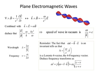
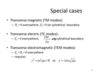
29. Nature of Electromagnetic Waves
• A general plane wave with angular frequency  travelling in the direction
of the wave vector k has the form
• Phase = 2  number of waves and so is a Lorentz invariant.
• Apply Maxwell’s equations
)]
(
exp[
)]
(
exp[ 0
0 x
k
t
i
B
B
x
k
t
i
E
E













 


i
t
k
i







B
E
k
B
E
B
k
E
k
B
E






























 0
0
Waves are transverse to the direction of propagation,
and and are mutually perpendicular
B
E


,
k

x
k
t






30. Plane
Electromagnetic Wave
30

31. Plane Electromagnetic Waves
E
c
B
k
t
E
c
B





2
2
1 














2
Frequency
k
2
Wavelength

 



2
that
deduce
with
Combined
kc
k
B
E
B
E
k









c
k

 

is
in vacuum
wave
of
speed
Reminder: The fact that is an
invariant tells us that
is a Lorentz 4-vector, the 4-Frequency vector.
Deduce frequency transforms as
x
k
t












 k
c

,

  v
c
v
c
k
v






 






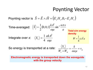
32. Waves in a Conducting Medium
• (Ohm’s Law) For a medium of conductivity ,
• Modified Maxwell:
• Put
E
j







D
t
E
E
t
E
j
H


















E
i
E
H
k
i






 



conduction
current
displacement
current
)]
(
exp[
)]
(
exp[ 0
0 x
k
t
i
B
B
x
k
t
i
E
E













 

4
0
8
-
12
0
7
10
57
.
2
1
.
2
,
10
3
:
Teflon
10
,
10
8
.
5
:
Copper












D
D






Dissipation
factor

33. Attenuation in a Good Conductor
   
   
  0
since
with
Combine
2
2































E
k
i
k
E
i
E
k
k
E
k
E
i
H
k
E
k
k
H
E
k
t
B
E





































E
i
E
H
k
i






 



For a good conductor D >> 1,  
i
k
i
k 




 1
2
, 2 





 
depth
-
skin
the
is
2
where
1
1
,
exp
exp
is
form
Wave





























 i
k
x
x
t
i copper.mov water.mov

34. Charge Density in a Conducting Material
• Inside a conductor (Ohm’s law)
• Continuity equation is
• Solution is
E
j




























t
E
t
j
t
0
0





 t
e
 0
So charge density decays exponentially with time. For a very
good conductor, charges flow instantly to the surface to form a
surface charge density and (for time varying fields) a surface
current. Inside a perfect conductor () E=H=0

35. Maxwell’s Equations in a Uniform Perfectly
Conducting Guide
   










 










 














0
2
2
2
2

























































H
E
E
H
i
E
E
E
E
i
t
D
H
H
i
t
B
E










z
y
x
Hollow metallic cylinder with perfectly
conducting boundary surfaces
Maxwell’s equations with time dependence exp(it) are:
Assume
)
(
)
(
)
,
(
)
,
,
,
(
)
,
(
)
,
,
,
(
z
t
i
z
t
i
e
y
x
H
t
z
y
x
H
e
y
x
E
t
z
y
x
E












Then   0
)
( 2
2
2










H
E
t 




 is the propagation constant
Can solve for the fields completely
in terms of Ez and Hz

36. Special cases
• Transverse magnetic (TM modes):
– Hz=0 everywhere, Ez=0 on cylindrical boundary
• Transverse electric (TE modes):
– Ez=0 everywhere, on cylindrical boundary
• Transverse electromagnetic (TEM modes):
– Ez=Hz=0 everywhere
– requires
36
0



n
Hz





 i



 or
0
2
2

37. Cut-off frequency, c
 c gives real solution for , so
attenuation only. No wave propagates: cut-
off modes.
 c gives purely imaginary solution for ,
and a wave propagates without attenuation.
 For a given frequency  only a finite number
of modes can propagate.
37







 

a
n
e
a
x
n
A
E
a
n
c
z
t
i
c











 
,
sin
,
1
2







a
n
a
n
c 


 For given frequency, convenient to
choose a s.t. only n=1 mode
occurs.
 
2
1
2
2
2
1
2
2
1
, 



















 c
c
k
ik

38. Propagated Electromagnetic Fields
From
 
 




































kz
t
a
x
n
a
n
A
H
H
kz
t
a
x
n
Ak
H
E
i
H
A
t
B
E
z
y
x











sin
cos
0
cos
sin
real,
is
assuming
,




38
z
x

39. Phase and group velocities in the simple wave guide
39
  



 

 2
1
2
2
c
k
Wave number:
wavelength
space
free
the
,
2
2








k
Wavelength:
velocity
space
-
free
than
larger
,
1




k
vp
Phase velocity:
 
velocity
space
-
free
than
smaller
1
2
2
2





 





k
dk
d
v
k g
c
Group velocity:

40. Calculation of Wave Properties
• If a=3 cm, cut-off frequency of lowest order mode is
• At 7 GHz, only the n=1 mode propagates and
GHz
5
03
.
0
2
10
3
2
1
2
8









a
f c
c
   
c
k
v
c
k
v
k
k
g
p
c




















1
8
1
8
1
8
9
2
1
2
2
2
1
2
2
ms
10
1
.
2
ms
10
3
.
4
cm
6
2
m
103
10
3
/
10
5
7
2








40



a
n
c 

41. Flow of EM energy along the simple guide
 
 
kz
t
a
x
n
A
a
n
H
H
E
k
H
kz
t
a
x
n
A
E
E
E
z
y
y
x
y
z
x

















sin
cos
,
0
,
cos
sin
,
0










2
2
2
2
2
2
2
2
0
2
2
0
2
since
8
1
4
1
energy
Magnetic
8
1
4
1
energy
Electric




































a
n
k
W
k
a
n
a
A
dx
H
W
a
A
dx
E
W
e
a
m
a
e


41
Fields (c) are:
Time-averaged energy:
Total e/m energy
density
a
A
W 2
4
1



42. Poynting Vector
42
Poynting vector is  
x
y
z
y H
E
H
E
H
E
S 


 ,
0
,



Time-averaged:  
a
x
n
kA
S


2
2
sin
1
,
0
,
0
2
1


Integrate over x:

2
4
1 akA
Sz 
So energy is transported at a rate: g
m
e
z
v
k
W
W
S


 
Electromagnetic energy is transported down the waveguide
with the group velocity
Total e/m energy
density
a
A
W 2
4
1

