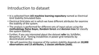
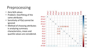
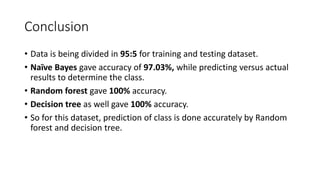
The document presents an analysis of electrical grid stability using a dataset from the UCI machine learning repository, focusing on classifying the stability into stable and unstable categories. Various machine learning methods, including Naïve Bayes, Random Forest, and Decision Tree, were employed, yielding high accuracy results, with Random Forest and Decision Tree achieving 100% accuracy. The study involves preprocessing data, attribute selection, and evaluating model performance through precision, recall, and F1 scores.

1. Electrical Grid Stability
Simulated Data Set analysis
using R
Ramandeep Kaur Bagri

2. Problem formulation
• This is classification/Regression problem, this presentation will only
cover classification of electrical grid stability into two classes;
1. Stable
2. Unstable

3. Introduction to dataset
• It is collected from UCI machine learning repository named as Electrical
Grid Stability Simulated Data.
• Electrical Grid data set in which we have different attributes for examine
the stability of the system.
• The analysis is performed for different sets of input values using the
methodology Naïve Bayes, Random forest and decision tree for classify
the system stability.
• Further, if you are interested about the dataset refer to; Schäfer,
Benjamin, et al. 'Taming instabilities in power grid networks by
decentralized control.
• We will examine the response of the system stability depends on 10,000
observations and 13 attributes, 1 classes attribute (stab).

4. Attributes Information
• Total - 14 predictive attributes, 1target attribute(2classes)
• tau[x] : Reaction time of participant (real from the range [0.5,10]s).
• p[x] : Nominal power consumed(negative)/produced(positive)(real).
• g[x] : Coefficient (gamma) proportional to price elasticity (real from
the range [0.05,1]s^-1).
• stab: The maximal real part of the characteristic equation root (if
positive - the system is linearly unstable)(real)
• stabf: The stability label of the system (stable/unstable)

5. Head of the dataset

6. Summary of dataset

7. Preprocessing
• Zero N/A values
• Problem: Overfitting of the
same attributes
• Sensitivity of P(x) cannot be
ignored
• Method of choosing attributes
is analyzing summary
characteristics, mean and
quartile values are considered.

8. Preprocessing Continue
• Null the following attributes by analyzing the summary characteristics:
• Tau4
• P3
• G2
• Considered attributes; summary (Talk about p4-p2);

9. Classes Distribution
• Distribution of classes:
• Stable
• Unstable

10. Relation between attributes (g1 p1 p2 stabf
tau2) and classes
• Attributes-g1 p1 p2 tau2, Class – Stable, Unstable
• Attributes-Tau 1 g1 p1, Class- Stable, Unstable
• Pink: Unstable
• Light Blue: Stable

11. Analyzing the both classes among attribute
• Pink - Unstable (Class)
• Blue - Stable (Class)
• G1 p2 p1 – Classes: Stable, Unstable • P1, Tau2, P2 – Classes: Stable, Unstable

12. Splitting the dataset
• Training Data Set: 95% [9091 11] • Testing Data Set: 5% [909 11]

13. Naïve Bayes Results
• Accuracy = 97.03%
• Precision [How many selected items are
relevant OR TP/(TP+FP)]= = 0.9558
• Recall [How many items are selected
relevant OR TP/TP+FN]= 0.9589
• F1 (Harmonic mean of precision and recall)=
(2 * 0.9558 * 0.9589) / (0.9558 + 0.9589) =
0.9573475

14. Random Forest Results
• Accuracy = 100%
• Precision [How many selected
items are relevant OR
TP/(TP+FP)]= 1
• Recall [How many items are
selected relevant OR TP/TP+FN]=
1
• F1 = (2 * 1* 1) / (1 + 1) = 1

15. Decision Tree Results
• Accuracy = 100%
• Precision [How many selected
items are relevant OR
TP/(TP+FP)]= 1
• Recall [How many items are
selected relevant OR TP/TP+FN]=
1
• F1 = (2 * 1 * 1) / (1 + 1) = 1

16. Conclusion
• Data is being divided in 95:5 for training and testing dataset.
• Naïve Bayes gave accuracy of 97.03%, while predicting versus actual
results to determine the class.
• Random forest gave 100% accuracy.
• Decision tree as well gave 100% accuracy.
• So for this dataset, prediction of class is done accurately by Random
forest and decision tree.