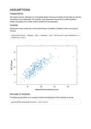
- The document analyzes a dataset relating body fat percentage to various measurements to find a predictor. - It finds that abdominal circumference has the highest correlation (0.81) to body fat percentage. A linear regression model is fitted with abdominal circumference predicting body fat percentage. - The model is found to be statistically significant and explains 66.21% of the variability in body fat percentage based on the abdominal circumference measurement.

1. MATH1324 Assignment 3
s3712731
2 June 2018
Introduction
We’re exploring a data set relating to body fat percentage, with the ultimate goal of finding an easily
measured predictor. The Brozek method for measuring body fat percentage is costly and time-
consuming, so identifying such a predictor could be financially beneficial. We first load the data,
then begin the four set tasks.
Bodydata <- read_excel("Body (2) Assignment 3 data.xlsx")
Bodydata$Sex <- factor(Bodydata$Sex, levels = c(1,0),labels = c("Male","Female"))
Task 1
The first task is to test whether there is a statistically significant difference between mean body fat
percentage for males and for females . The result of this test could inform our decision
to keep the data split, or combine it in our future analysis.
We’ll be using a two-sample t-test to determine whether there is a difference.
The null hypothesis is that the mean body fat for males and females are equal:
The alternative hypothesis is that there is indeed a difference:
We create subsets of the data corresponding to males and to females.
Bodydata_male <- subset(Bodydata, subset=Sex =="Male") #Subset male data
Bodydata_female <- subset(Bodydata, subset=Sex =="Female") #Subset male data
Before conducting the test, we need to consider our assumptions.
Normality
Since there are 92 females and 160 males in the sample, and both these numbers are large
(greater than 30), we know by the Central Limit Theorem that the sampling distribution of the mean
will be approximately normally distributed.
Homogeneity of Variance
To test the homogeneity of variance assumption, we conduct the Levene’s Test.
( )μM ( )μF
: − = 0H0 μM μF
: − ≠ 0HA μM μF

2. leveneTest(BFP_Brozek ~ Sex, data = Bodydata)
## Levene's Test for Homogeneity of Variance (center = median)
## Df F value Pr(>F)
## group 1 2.1974 0.1395
## 250
The p-value of 0.1395 is greater than 0.05, and so we fail to reject the null hypothesis of equal
variance. Therefore, we can proceed with the two-sample t-test under the assumption of equal
variance.
Two-sample t-test (assuming equal variance)
t.test(BFP_Brozek ~ Sex, data = Bodydata, var.equal=TRUE, alternative="two.sided")
##
## Two Sample t-test
##
## data: BFP_Brozek by Sex
## t = -0.75154, df = 250, p-value = 0.453
## alternative hypothesis: true difference in means is not equal to 0
## 95 percent confidence interval:
## -2.761898 1.236246
## sample estimates:
## mean in group Male mean in group Female
## 18.66000 19.42283
The p-value of 0.453 is greater than the 0.05 level of significance, so our test is not statistically
significant. It is safe to assume that the mean body fat percentage for males and for females are
equal, and we will consider them together for the following tasks.
Task 2
The second task is to estimate the 99% confidence interval for the mean body fat percentage in the
population. Because of the large sample size (252) and the Central Limit Theorem, we can use a
regular CI formula with an adjustment to account for the fact that the population standard deviation
is unknown. We use the sample standard deviation, and a t-distribution with df = 252 - 1. This can
be done simply with the following R code:
confint(t.test( ~ BFP_Brozek, data = Bodydata, conf.level=0.99))
## mean of x lower upper level
## 1 18.93849 17.67119 20.20579 0.99
Our 99% confidence interval for the population mean body fat percentage is (17.67119, 20.20579).
This means that 99% of confidence intervals constructed in this fashion will contain the population
mean body fat percentage.

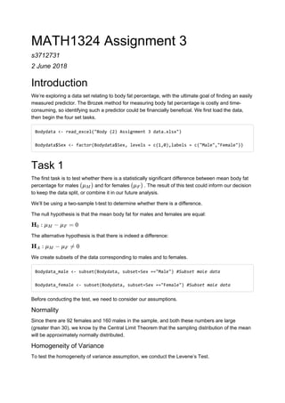
3. Task 3
In Task 3, we are asked to test the claim by researchers that the average body fat percentage is
less than 12.5. This claim corresponds to the mathematical statement that , which is
equivalent to since the probability that is precisely 12.5 is zero.
For simplicity we can take the following as our null and alternative hypotheses:
This is justified because statistically significant support for our alternative hypothesis will lead to a
rejection of the statement made by the researchers.
We use the p-value approach.
m<-mean(Bodydata$BFP_Brozek)
mu<-12.5
s<-sd(Bodydata$BFP_Brozek)
n<-length(Bodydata$BFP_Brozek)
se<-s/sqrt(n)
t<-(m-mu)/se
t
## [1] 13.18666
pt(t,df=n-1, lower.tail=FALSE)
## [1] 7.994808e-31
This p-value is extremely small and we would round it to 0.001. It is certainly far smaller than 0.05,
and so the result is statistically significant. In other words, our data gives statistically significant
evidence that the claim average body fat percentage is less than 12.5 is incorrect, because the
probability of observing our sample statistic under the assumption that the claim is true is near zero.
Task 4
In Task 4 we seek to investigate a means of predicting body fat percentage using body
circumference data. The data set includes ten different circumference measurements, and our first
step is to identify the single best predictor.
The Pearson Correlation Coefficient was used to make this identification. For each of the ten
different circumference measurements, the code below was used to measure the correlation with
body fat percentage. The results were:
Circumference Measurement (cm) Pearson Correlation with BFP
Neck 0.49
Chest 0.7
μ < 12.5
μ ≤ 12.5 μ
: μ = 12.5H0
: μ > 12.5HA

4. Circumference Measurement (cm) Pearson Correlation with BFP
Abdomen 0.81
Hip 0.63
Thigh 0.56
Knee 0.51
Ankle 0.27
Biceps 0.49
Forearm 0.36
Wrist 0.35
All of the measurements showed a positive correlation with body fat percentage, but the
circumference of the Abdomen showed the highest correlation and is therefore the single best
predictor.
bivariate<-as.matrix(select(Bodydata, BFP_Brozek,Abdomen))
rcorr(bivariate, type = "pearson")
## BFP_Brozek Abdomen
## BFP_Brozek 1.00 0.81
## Abdomen 0.81 1.00
##
## n= 252
##
##
## P
## BFP_Brozek Abdomen
## BFP_Brozek 0
## Abdomen 0
Now that we’ve identified the single best predictor of body fat percentage, we can fit a linear
regression model:
BFPBrozekmodel <- lm(BFP_Brozek ~ Abdomen, data = Bodydata)
msummary(BFPBrozekmodel)
## Estimate Std. Error t value Pr(>|t|)
## (Intercept) -35.19661 2.46229 -14.29 <2e-16 ***
## Abdomen 0.58489 0.02643 22.13 <2e-16 ***
##
## Residual standard error: 4.514 on 250 degrees of freedom
## Multiple R-squared: 0.6621, Adjusted R-squared: 0.6608
## F-statistic: 489.9 on 1 and 250 DF, p-value: < 2.2e-16
Before reporting on this model, we need to test the assumptions that its validity relies on.

5. ASSUMPTIONS
Independence
We need to assume, although it is not explicitly stated in the documentation for the data set, that the
observations are independent. For example, each observation should be of a different person.
Ideally, the people are a simple random sample from the population.
Linearity
Observation of the scatter plot, and the high Pearson Corellation Coeffcient, allow us to assume
linearity.
xyplot(BFP_Brozek ~ Abdomen, data = Bodydata, ylab ="BFP_Brozek",xlab="Abdominal Ci
rcumference (cm)")
Normality of residuals
The following plot allows us to visualise whether the distribution of the residuals is normal:
qqPlot(BFPBrozekmodel$residuals, dist="norm")

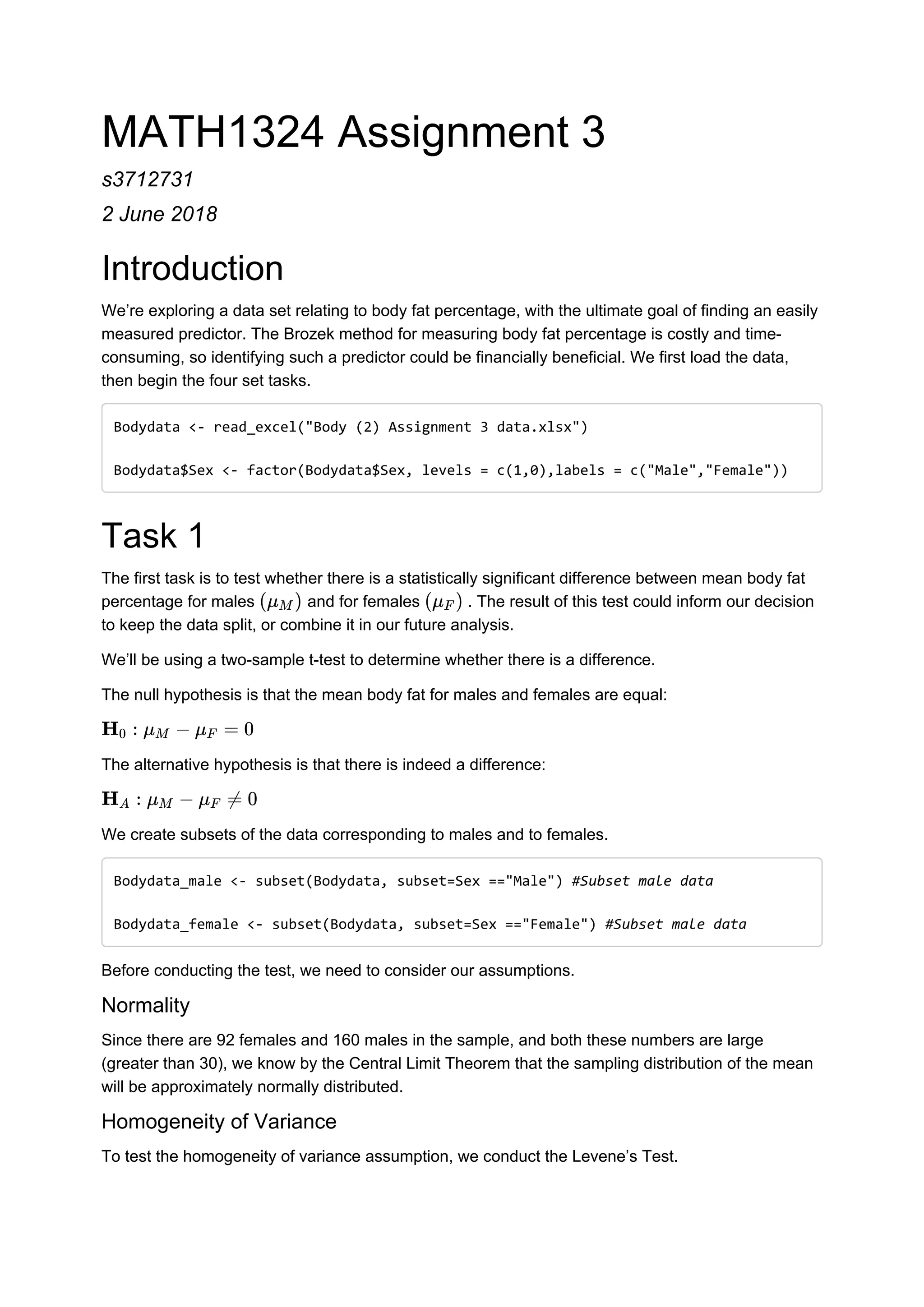
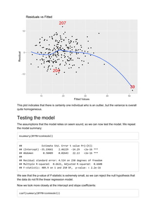
6. ## [1] 39 207
There don’t appear to be any major deviations from normality.
Homoscedasticity
Homoscedasticity can be observed by looking at a scatter plot of predicted values against residuals.
mplot(BFPBrozekmodel, 1)
## [[1]]
## `geom_smooth()` using method = 'loess'

7. This plot indicates that there is certainly one individual who is an outlier, but the variance is overall
quite homogeneous.
Testing the model
The assumptions that the model relies on seem sound, so we can now test the model. We repeat
the model summary:
msummary(BFPBrozekmodel)
## Estimate Std. Error t value Pr(>|t|)
## (Intercept) -35.19661 2.46229 -14.29 <2e-16 ***
## Abdomen 0.58489 0.02643 22.13 <2e-16 ***
##
## Residual standard error: 4.514 on 250 degrees of freedom
## Multiple R-squared: 0.6621, Adjusted R-squared: 0.6608
## F-statistic: 489.9 on 1 and 250 DF, p-value: < 2.2e-16
We see that the p-value of F-statistic is extremely small, so we can reject the null hypothesis that
the data do not fit the linear regression model.
Now we look more closely at the intercept and slope coefficients:
coef(summary(BFPBrozekmodel))

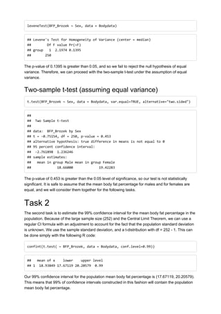
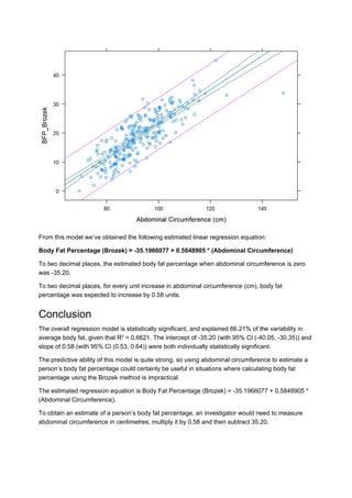
8. ## Estimate Std. Error t value Pr(>|t|)
## (Intercept) -35.1966077 2.46229413 -14.29423 2.790180e-34
## Abdomen 0.5848905 0.02642528 22.13375 7.706457e-61
The null and alternative hypotheses for the intecept are:
We compute the two-tailed p-value for this constant:
2*pt(-14.29423,252-2,lower.tail=TRUE)
## [1] 2.790261e-34
Since this value is less than 0.05, the intercept is statistically significant.
The null and alternative hyptheses for the slope are:
We compute the two-tailed p-value for this slope:
2*pt(22.13375,252-2,lower.tail=FALSE)
## [1] 7.706439e-61
Again, the p-value is much less than 0.05 so the slope is statistically significant.
95% Confidence Intervals for intercept and slope can also be calculated:
confint(BFPBrozekmodel)
## 2.5 % 97.5 %
## (Intercept) -40.046092 -30.3471234
## Abdomen 0.532846 0.6369351
The following plot summarises the linear relationship between Abdominal Circumference and Body
Fat Percentage as measured by the Brozek method.
xyplot(BFP_Brozek ~ Abdomen, data = Bodydata, ylab ="BFP_Brozek", xlab="Abdominal C
ircumference (cm)", panel=panel.lmbands)
α
: α = 0H0
: α ≠ 0HA
β
: β = 0H0
: β ≠ 0HA

9. From this model we’ve obtained the following estimated linear regression equation:
Body Fat Percentage (Brozek) = -35.1966077 + 0.5848905 * (Abdominal Circumference)
To two decimal places, the estimated body fat percentage when abdominal circumference is zero
was -35.20.
To two decimal places, for every unit increase in abdominal circumference (cm), body fat
percentage was expected to increase by 0.58 units.
Conclusion
The overall regression model is statistically significant, and explained 66.21% of the variability in
average body fat, given that R = 0.6621. The intercept of -35.20 (with 95% CI (-40.05, -30.35)) and
slope of 0.58 (with 95% CI (0.53, 0.64)) were both individually statistically significant.
The predictive ability of this model is quite strong, so using abdominal circumference to estimate a
person’s body fat percentage could certainly be useful in situations where calculating body fat
percentage using the Brozek method is impractical.
The estimated regression equation is Body Fat Percentage (Brozek) = -35.1966077 + 0.5848905 *
(Abdominal Circumference).
To obtain an estimate of a person’s body fat percentage, an investigator would need to measure
abdominal circumference in centimetres, multiply it by 0.58 and then subtract 35.20.
2