Download as PDF, PPTX


![4
Electric Field Strength [V/m]
Magnetic Field Strength [A/m]
Electric Volume Current Density [A/m²]
Magnetic Volume Current Density [V/m²]
J HE M
DEFINITIONS](https://image.slidesharecdn.com/gibdko2wq5lyygqy69na-signature-ee8c0ba1fb28ead38883579b44e12ea87f9eb78d6bc8123d62b406436d35857a-poli-140914173114-phpapp01/85/Ece5318-ch3-4-320.jpg)
![5
DEFINITIONS
(CONT)
Electric Vector Potential [Wb/m]
Electrical Scalar Potential [V]
Magnetic Vector Potential [A-sec/m]
Magnetic Scalar Potential [A]
A F m e](https://image.slidesharecdn.com/gibdko2wq5lyygqy69na-signature-ee8c0ba1fb28ead38883579b44e12ea87f9eb78d6bc8123d62b406436d35857a-poli-140914173114-phpapp01/85/Ece5318-ch3-5-320.jpg)

![8
The total fields are
FHEEEAFA 11j
(solutions derived in Sect. 3.5)
(also for surface and linear currents)
FFAEAHHH j11
[3-29a]
[3-30a]](https://image.slidesharecdn.com/gibdko2wq5lyygqy69na-signature-ee8c0ba1fb28ead38883579b44e12ea87f9eb78d6bc8123d62b406436d35857a-poli-140914173114-phpapp01/85/Ece5318-ch3-8-320.jpg)


![13
RECIPROCITY
(CONT)
Lorentz Reciprocity Theorem
(also valid for fields away from finite sources – far fields)
each integral is called a “REACTION”
of fields (E, H ) to the sources (J, M )
' 1212' 2121dvdvvv MHJEMHJE
[3-66]](https://image.slidesharecdn.com/gibdko2wq5lyygqy69na-signature-ee8c0ba1fb28ead38883579b44e12ea87f9eb78d6bc8123d62b406436d35857a-poli-140914173114-phpapp01/85/Ece5318-ch3-13-320.jpg)


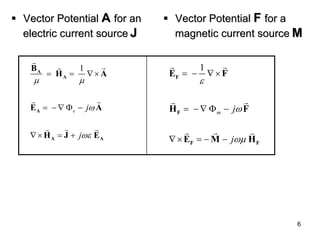
This document discusses vector potentials and radiation integrals used in antenna engineering. It defines key terms like electric and magnetic vector potentials, electric and magnetic fields, and electric and magnetic current densities. It describes how vector potentials are used to simplify calculating radiated fields from sources. It also summarizes concepts like far field radiation patterns, duality between electric and magnetic fields, and reciprocity theorems relating fields and sources.


