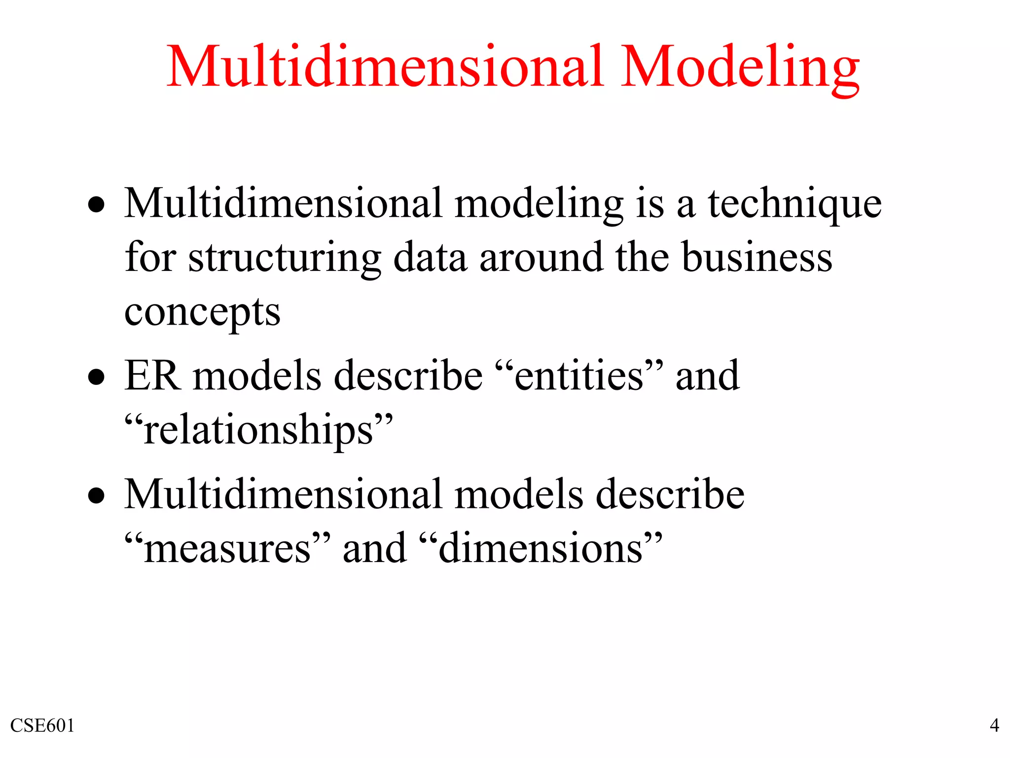
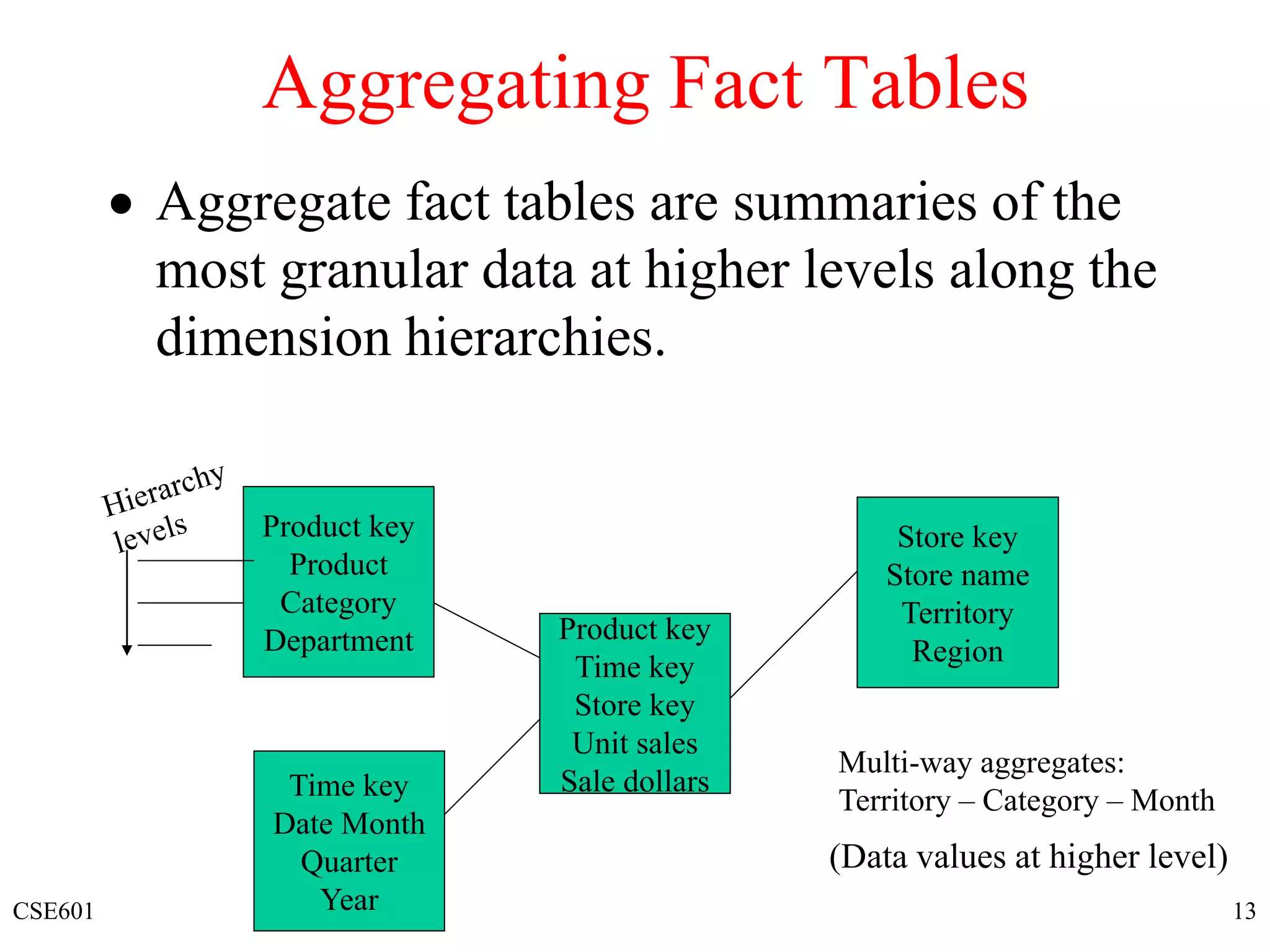
CSE601 1
Warehouse Models & Operators
 Data Models
 relations
 stars & snowflakes
 cubes
 Operators
 slice & dice
 roll-up, drill down
 pivoting
 other
CSE601 2
Multi-Dimensional Data
 Measures - numerical (and additive) data
being tracked in business, can be analyzed
and examined
 Dimensions - business parameters that
define a transaction, relatively static data
such as lookup or reference tables
 Example: Analyst may want to view sales
data (measure) by geography, by time, and
by product (dimensions)
CSE601 3
The Multi-Dimensional Model
“Sales by product line over the past six months”
“Sales by store between 1990 and 1995”
Prod Code Time Code Store Code Sales Qty
Store Info
Product Info
Time Info
. . .
Numerical Measures
Key columns joining fact table
to dimension tables
Fact table for
measures
Dimension tables
CSE601 4
Multidimensional Modeling
 Multidimensional modeling is a technique
for structuring data around the business
concepts
 ER models describe “entities” and
“relationships”
 Multidimensional models describe
“measures” and “dimensions”
CSE601 5
Dimensional Modeling
 Dimensions are organized into hierarchies
 E.g., Time dimension: days  weeks  quarters
 E.g., Product dimension: product  product line 
brand
 Dimensions have attributes
Time Store
Date
Month
Year
StoreID
City
State
Country
Region
CSE601 6
Dimension Hierarchies
Store Dimension Product Dimension
District
Region
Total
Brand
Manufacturer
Total
Stores Products
CSE601 7
Schema Design
 Most data warehouses use a star schema to represent multi-
dimensional model.
 Each dimension is represented by a dimension table that
describes it.
 A fact table connects to all dimension tables with a
multiple join. Each tuple in the fact table consists of a
pointer to each of the dimension tables that provide its
multi-dimensional coordinates and stores measures for
those coordinates.
 The links between the fact table in the center and the
dimension tables in the extremities form a shape like a star.
CSE601 8
Star Schema (in RDBMS)
CSE601 9
Star Schema Example
CSE601 10
Star Schema
with Sample
Data
CSE601 11
The “Classic” Star Schema
 A relational model with a one-to-many relationship
between dimension table and fact table.
 A single fact table, with detail and summary data
 Fact table primary key has only one key column per
dimension
 Each dimension is a single table, highly denormalized
 Benefits: Easy to understand, intuitive mapping between the
business entities, easy to define hierarchies, reduces # of physical
joins, low maintenance, very simple metadata
 Drawbacks: Summary data in the fact table yields poorer
performance for summary levels, huge dimension tables a problem
CSE601 12
Need for Aggregates
 Sizes of typical tables:
 Time dimension: 5 years x 365 days = 1825
 Store dimension: 300 stores reporting daily sales
 Production dimension: 40,000 products in each store
(about 4000 sell in each store daily)
 Maximum number of base fact table records: 2 billion
(lowest level of detail)
 A query involving 1 brand, all store, 1 year:
retrieve/summarize over 7 million fact table rows.
CSE601 13
Aggregating Fact Tables
 Aggregate fact tables are summaries of the
most granular data at higher levels along the
dimension hierarchies.
Product key
Time key
Store key
Unit sales
Sale dollars
Product key
Product
Category
Department
Store key
Store name
Territory
Region
Time key
Date Month
Quarter
Year
Multi-way aggregates:
Territory – Category – Month
(Data values at higher level)
CSE601 14
The “Fact Constellation” Schema
Dollars
Units
Price
District Fact Table
District_ID
PRODUCT_KE
Y
PERIOD_KEY
Dollars
Units
Price
Region Fact Table
Region_ID
PRODUCT_KEY
PERIOD_KEY
PERIOD KEY
Store Dimension Time Dimension
Product Dimension
STOREKEY
PRODUCTKEY
PERIOD KEY
Dollars
Units
Price
Period Desc
Year
Quarter
Month
Day
Current Flag
Sequence
Fact Table
PRODUCTKEY
Store Description
City
State
District ID
District Desc.
Region_ID
Region Desc.
Regional Mgr.
Product Desc.
Brand
Color
Size
Manufacturer
STORE KEY
CSE601 15
Aggregate Fact Tables
Product key
Time key
Store key
Unit sales
Sale dollars
Category key
Time key
Store key
Unit sales
Sales dollars
Product key
Product
Category
Department
Time key
Date
Month
Quarter
Year
Store key
Store name
Territory
Region
Category key
Category
Department
Base table
Sales facts
Store
Product
Time
One-way aggregate
Sale facts
Dimension
Derived from Product
Category
CSE601 16
Families of Stars
Dimension
table
Fact table
Fact table
Fact table
Dimension
table
Dimension
table
Dimension
table
Dimension
table
Dimension
table
Dimension
table
Dimension
table
CSE601 17
Snowflake Schema
 Snowflake schema is a type of star schema
but a more complex model.
 “Snowflaking” is a method of normalizing
the dimension tables in a star schema.
 The normalization eliminates redundancy.
 The result is more complex queries and
reduced query performance.
CSE601 18
Sales: Snowflake Schema
Salesrep key
Salesperson name
Territory key
Product key
Time key
Customer key
….
Product key
Product name
Product code
Brand key
Brand key
Brand name
Category key
Category key
Product category
Territory key
Territory name
Region key
Region key
Region name
Sales fact
Product
Salesrep
CSE601 19
Snowflaking
 The attributes with low cardinality in each
original dimension table are removed to
form separate tables. These new tables are
linked back to the original dimension table
through artificial keys.
Product key
Product name
Product code
Brand key
Brand key
Brand name
Category key
Category key
Product category
CSE601 20
Snowflake Schema
 Advantages:
 Small saving in storage space
 Normalized structures are easier to update and maintain
 Disadvantages:
 Schema less intuitive and end-users are put off by the
complexity
 Ability to browse through the contents difficult
 Degrade query performance because of additional joins
CSE601 21
What is the Best Design?
 Performance benchmarking can be used to
determine what is the best design.
 Snowflake schema: easier to maintain dimension
tables when dimension tables are very large
(reduce overall space). It is not generally
recommended in a data warehouse environment.
 Star schema: more effective for data cube
browsing (less joins): can affect performance.
CSE601 22
Aggregates
sale prodId storeId date amt
p1 s1 1 12
p2 s1 1 11
p1 s3 1 50
p2 s2 1 8
p1 s1 2 44
p1 s2 2 4
 Add up amounts for day 1
 In SQL: SELECT sum(amt) FROM SALE
WHERE date = 1
81
CSE601 23
Aggregates
 Add up amounts by day
 In SQL: SELECT date, sum(amt) FROM SALE
GROUP BY date
ans date sum
1 81
2 48
sale prodId storeId date amt
p1 s1 1 12
p2 s1 1 11
p1 s3 1 50
p2 s2 1 8
p1 s1 2 44
p1 s2 2 4
CSE601 24
Another Example
 Add up amounts by day, product
 In SQL: SELECT date, sum(amt) FROM SALE
GROUP BY date, prodId
sale prodId date amt
p1 1 62
p2 1 19
p1 2 48
drill-down
rollup
sale prodId storeId date amt
p1 s1 1 12
p2 s1 1 11
p1 s3 1 50
p2 s2 1 8
p1 s1 2 44
p1 s2 2 4
CSE601 25
Aggregates
 Operators: sum, count, max, min,
median, ave
 “Having” clause
 Using dimension hierarchy
 average by region (within store)
 maximum by month (within date)
CSE601 26
Data Cube
sale prodId storeId amt
p1 s1 12
p2 s1 11
p1 s3 50
p2 s2 8
s1 s2 s3
p1 12 50
p2 11 8
Fact table view:
Multi-dimensional cube:
dimensions = 2
CSE601 27
3-D Cube
dimensions = 3
Multi-dimensional cube:
Fact table view:
sale prodId storeId date amt
p1 s1 1 12
p2 s1 1 11
p1 s3 1 50
p2 s2 1 8
p1 s1 2 44
p1 s2 2 4
day 2 s1 s2 s3
p1 44 4
p2 s1 s2 s3
p1 12 50
p2 11 8
day 1
CSE601 28
Example
Product
Time
M T W Th F S S
Juice
Milk
Coke
Cream
Soap
Bread
NY
SF
LA
10
34
56
32
12
56
56 units of bread sold in LA on M
Dimensions:
Time, Product, Store
Attributes:
Product (upc, price, …)
Store …
…
Hierarchies:
Product  Brand  …
Day  Week  Quarter
Store  Region  Country
roll-up to week
roll-up to brand
roll-up to region
CSE601 29
Cube Aggregation: Roll-up
day 2 s1 s2 s3
p1 44 4
p2 s1 s2 s3
p1 12 50
p2 11 8
day 1
s1 s2 s3
p1 56 4 50
p2 11 8
s1 s2 s3
sum 67 12 50
sum
p1 110
p2 19
129
. . .
drill-down
rollup
Example: computing sums
CSE601 30
Cube Operators for Roll-up
day 2 s1 s2 s3
p1 44 4
p2 s1 s2 s3
p1 12 50
p2 11 8
day 1
s1 s2 s3
p1 56 4 50
p2 11 8
s1 s2 s3
sum 67 12 50
sum
p1 110
p2 19
129
. . .
sale(s1,*,*)
sale(*,*,*)
sale(s2,p2,*)
CSE601 31
s1 s2 s3 *
p1 56 4 50 110
p2 11 8 19
* 67 12 50 129
Extended Cube
day 2 s1 s2 s3 *
p1 44 4 48
p2
* 44 4 48
s1 s2 s3 *
p1 12 50 62
p2 11 8 19
* 23 8 50 81
day 1
*
sale(*,p2,*)
CSE601 32
Aggregation Using Hierarchies
region A region B
p1 56 54
p2 11 8
store
region
country
(store s1 in Region A;
stores s2, s3 in Region B)
day 2 s1 s2 s3
p1 44 4
p2 s1 s2 s3
p1 12 50
p2 11 8
day 1
CSE601 33
Slicing
day 2 s1 s2 s3
p1 44 4
p2 s1 s2 s3
p1 12 50
p2 11 8
day 1
s1 s2 s3
p1 12 50
p2 11 8
TIME = day 1
CSE601 34
Products
d1 d2
Store s1 Electronics $5.2
Toys $1.9
Clothing $2.3
Cosmetics $1.1
Store s2 Electronics $8.9
Toys $0.75
Clothing $4.6
Cosmetics $1.5
Products
Store s1 Store s2
Store s1 Electronics $5.2 $8.9
Toys $1.9 $0.75
Clothing $2.3 $4.6
Cosmetics $1.1 $1.5
Store s2 Electronics
Toys
Clothing
($ millions)
d1
Sales
($ millions)
Time
Sales
Slicing &
Pivoting
CSE601 35
Summary of Operations
 Aggregation (roll-up)
 aggregate (summarize) data to the next higher dimension
element
 e.g., total sales by city, year  total sales by region, year
 Navigation to detailed data (drill-down)
 Selection (slice) defines a subcube
 e.g., sales where city =‘Gainesville’ and date = ‘1/15/90’
 Calculation and ranking
 e.g., top 3% of cities by average income
 Visualization operations (e.g., Pivot)
 Time functions
 e.g., time average
CSE601 36
Query & Analysis Tools
 Query Building
 Report Writers (comparisons, growth, graphs,…)
 Spreadsheet Systems
 Web Interfaces
 Data Mining

DW-lecture2.ppt

  • 1.
    CSE601 1 Warehouse Models& Operators  Data Models  relations  stars & snowflakes  cubes  Operators  slice & dice  roll-up, drill down  pivoting  other
  • 2.
    CSE601 2 Multi-Dimensional Data Measures - numerical (and additive) data being tracked in business, can be analyzed and examined  Dimensions - business parameters that define a transaction, relatively static data such as lookup or reference tables  Example: Analyst may want to view sales data (measure) by geography, by time, and by product (dimensions)
  • 3.
    CSE601 3 The Multi-DimensionalModel “Sales by product line over the past six months” “Sales by store between 1990 and 1995” Prod Code Time Code Store Code Sales Qty Store Info Product Info Time Info . . . Numerical Measures Key columns joining fact table to dimension tables Fact table for measures Dimension tables
  • 4.
    CSE601 4 Multidimensional Modeling Multidimensional modeling is a technique for structuring data around the business concepts  ER models describe “entities” and “relationships”  Multidimensional models describe “measures” and “dimensions”
  • 5.
    CSE601 5 Dimensional Modeling Dimensions are organized into hierarchies  E.g., Time dimension: days  weeks  quarters  E.g., Product dimension: product  product line  brand  Dimensions have attributes Time Store Date Month Year StoreID City State Country Region
  • 6.
    CSE601 6 Dimension Hierarchies StoreDimension Product Dimension District Region Total Brand Manufacturer Total Stores Products
  • 7.
    CSE601 7 Schema Design Most data warehouses use a star schema to represent multi- dimensional model.  Each dimension is represented by a dimension table that describes it.  A fact table connects to all dimension tables with a multiple join. Each tuple in the fact table consists of a pointer to each of the dimension tables that provide its multi-dimensional coordinates and stores measures for those coordinates.  The links between the fact table in the center and the dimension tables in the extremities form a shape like a star.
  • 8.
  • 9.
  • 10.
  • 11.
    CSE601 11 The “Classic”Star Schema  A relational model with a one-to-many relationship between dimension table and fact table.  A single fact table, with detail and summary data  Fact table primary key has only one key column per dimension  Each dimension is a single table, highly denormalized  Benefits: Easy to understand, intuitive mapping between the business entities, easy to define hierarchies, reduces # of physical joins, low maintenance, very simple metadata  Drawbacks: Summary data in the fact table yields poorer performance for summary levels, huge dimension tables a problem
  • 12.
    CSE601 12 Need forAggregates  Sizes of typical tables:  Time dimension: 5 years x 365 days = 1825  Store dimension: 300 stores reporting daily sales  Production dimension: 40,000 products in each store (about 4000 sell in each store daily)  Maximum number of base fact table records: 2 billion (lowest level of detail)  A query involving 1 brand, all store, 1 year: retrieve/summarize over 7 million fact table rows.
  • 13.
    CSE601 13 Aggregating FactTables  Aggregate fact tables are summaries of the most granular data at higher levels along the dimension hierarchies. Product key Time key Store key Unit sales Sale dollars Product key Product Category Department Store key Store name Territory Region Time key Date Month Quarter Year Multi-way aggregates: Territory – Category – Month (Data values at higher level)
  • 14.
    CSE601 14 The “FactConstellation” Schema Dollars Units Price District Fact Table District_ID PRODUCT_KE Y PERIOD_KEY Dollars Units Price Region Fact Table Region_ID PRODUCT_KEY PERIOD_KEY PERIOD KEY Store Dimension Time Dimension Product Dimension STOREKEY PRODUCTKEY PERIOD KEY Dollars Units Price Period Desc Year Quarter Month Day Current Flag Sequence Fact Table PRODUCTKEY Store Description City State District ID District Desc. Region_ID Region Desc. Regional Mgr. Product Desc. Brand Color Size Manufacturer STORE KEY
  • 15.
    CSE601 15 Aggregate FactTables Product key Time key Store key Unit sales Sale dollars Category key Time key Store key Unit sales Sales dollars Product key Product Category Department Time key Date Month Quarter Year Store key Store name Territory Region Category key Category Department Base table Sales facts Store Product Time One-way aggregate Sale facts Dimension Derived from Product Category
  • 16.
    CSE601 16 Families ofStars Dimension table Fact table Fact table Fact table Dimension table Dimension table Dimension table Dimension table Dimension table Dimension table Dimension table
  • 17.
    CSE601 17 Snowflake Schema Snowflake schema is a type of star schema but a more complex model.  “Snowflaking” is a method of normalizing the dimension tables in a star schema.  The normalization eliminates redundancy.  The result is more complex queries and reduced query performance.
  • 18.
    CSE601 18 Sales: SnowflakeSchema Salesrep key Salesperson name Territory key Product key Time key Customer key …. Product key Product name Product code Brand key Brand key Brand name Category key Category key Product category Territory key Territory name Region key Region key Region name Sales fact Product Salesrep
  • 19.
    CSE601 19 Snowflaking  Theattributes with low cardinality in each original dimension table are removed to form separate tables. These new tables are linked back to the original dimension table through artificial keys. Product key Product name Product code Brand key Brand key Brand name Category key Category key Product category
  • 20.
    CSE601 20 Snowflake Schema Advantages:  Small saving in storage space  Normalized structures are easier to update and maintain  Disadvantages:  Schema less intuitive and end-users are put off by the complexity  Ability to browse through the contents difficult  Degrade query performance because of additional joins
  • 21.
    CSE601 21 What isthe Best Design?  Performance benchmarking can be used to determine what is the best design.  Snowflake schema: easier to maintain dimension tables when dimension tables are very large (reduce overall space). It is not generally recommended in a data warehouse environment.  Star schema: more effective for data cube browsing (less joins): can affect performance.
  • 22.
    CSE601 22 Aggregates sale prodIdstoreId date amt p1 s1 1 12 p2 s1 1 11 p1 s3 1 50 p2 s2 1 8 p1 s1 2 44 p1 s2 2 4  Add up amounts for day 1  In SQL: SELECT sum(amt) FROM SALE WHERE date = 1 81
  • 23.
    CSE601 23 Aggregates  Addup amounts by day  In SQL: SELECT date, sum(amt) FROM SALE GROUP BY date ans date sum 1 81 2 48 sale prodId storeId date amt p1 s1 1 12 p2 s1 1 11 p1 s3 1 50 p2 s2 1 8 p1 s1 2 44 p1 s2 2 4
  • 24.
    CSE601 24 Another Example Add up amounts by day, product  In SQL: SELECT date, sum(amt) FROM SALE GROUP BY date, prodId sale prodId date amt p1 1 62 p2 1 19 p1 2 48 drill-down rollup sale prodId storeId date amt p1 s1 1 12 p2 s1 1 11 p1 s3 1 50 p2 s2 1 8 p1 s1 2 44 p1 s2 2 4
  • 25.
    CSE601 25 Aggregates  Operators:sum, count, max, min, median, ave  “Having” clause  Using dimension hierarchy  average by region (within store)  maximum by month (within date)
  • 26.
    CSE601 26 Data Cube saleprodId storeId amt p1 s1 12 p2 s1 11 p1 s3 50 p2 s2 8 s1 s2 s3 p1 12 50 p2 11 8 Fact table view: Multi-dimensional cube: dimensions = 2
  • 27.
    CSE601 27 3-D Cube dimensions= 3 Multi-dimensional cube: Fact table view: sale prodId storeId date amt p1 s1 1 12 p2 s1 1 11 p1 s3 1 50 p2 s2 1 8 p1 s1 2 44 p1 s2 2 4 day 2 s1 s2 s3 p1 44 4 p2 s1 s2 s3 p1 12 50 p2 11 8 day 1
  • 28.
    CSE601 28 Example Product Time M TW Th F S S Juice Milk Coke Cream Soap Bread NY SF LA 10 34 56 32 12 56 56 units of bread sold in LA on M Dimensions: Time, Product, Store Attributes: Product (upc, price, …) Store … … Hierarchies: Product  Brand  … Day  Week  Quarter Store  Region  Country roll-up to week roll-up to brand roll-up to region
  • 29.
    CSE601 29 Cube Aggregation:Roll-up day 2 s1 s2 s3 p1 44 4 p2 s1 s2 s3 p1 12 50 p2 11 8 day 1 s1 s2 s3 p1 56 4 50 p2 11 8 s1 s2 s3 sum 67 12 50 sum p1 110 p2 19 129 . . . drill-down rollup Example: computing sums
  • 30.
    CSE601 30 Cube Operatorsfor Roll-up day 2 s1 s2 s3 p1 44 4 p2 s1 s2 s3 p1 12 50 p2 11 8 day 1 s1 s2 s3 p1 56 4 50 p2 11 8 s1 s2 s3 sum 67 12 50 sum p1 110 p2 19 129 . . . sale(s1,*,*) sale(*,*,*) sale(s2,p2,*)
  • 31.
    CSE601 31 s1 s2s3 * p1 56 4 50 110 p2 11 8 19 * 67 12 50 129 Extended Cube day 2 s1 s2 s3 * p1 44 4 48 p2 * 44 4 48 s1 s2 s3 * p1 12 50 62 p2 11 8 19 * 23 8 50 81 day 1 * sale(*,p2,*)
  • 32.
    CSE601 32 Aggregation UsingHierarchies region A region B p1 56 54 p2 11 8 store region country (store s1 in Region A; stores s2, s3 in Region B) day 2 s1 s2 s3 p1 44 4 p2 s1 s2 s3 p1 12 50 p2 11 8 day 1
  • 33.
    CSE601 33 Slicing day 2s1 s2 s3 p1 44 4 p2 s1 s2 s3 p1 12 50 p2 11 8 day 1 s1 s2 s3 p1 12 50 p2 11 8 TIME = day 1
  • 34.
    CSE601 34 Products d1 d2 Stores1 Electronics $5.2 Toys $1.9 Clothing $2.3 Cosmetics $1.1 Store s2 Electronics $8.9 Toys $0.75 Clothing $4.6 Cosmetics $1.5 Products Store s1 Store s2 Store s1 Electronics $5.2 $8.9 Toys $1.9 $0.75 Clothing $2.3 $4.6 Cosmetics $1.1 $1.5 Store s2 Electronics Toys Clothing ($ millions) d1 Sales ($ millions) Time Sales Slicing & Pivoting
  • 35.
    CSE601 35 Summary ofOperations  Aggregation (roll-up)  aggregate (summarize) data to the next higher dimension element  e.g., total sales by city, year  total sales by region, year  Navigation to detailed data (drill-down)  Selection (slice) defines a subcube  e.g., sales where city =‘Gainesville’ and date = ‘1/15/90’  Calculation and ranking  e.g., top 3% of cities by average income  Visualization operations (e.g., Pivot)  Time functions  e.g., time average
  • 36.
    CSE601 36 Query &Analysis Tools  Query Building  Report Writers (comparisons, growth, graphs,…)  Spreadsheet Systems  Web Interfaces  Data Mining