1. Child Development, January/February 2010, Volume 81, Number 1, Pages 306–325
Early-Childhood Poverty and Adult Attainment, Behavior, and Health
Greg J. Duncan
Kathleen M. Ziol-Guest
University of California Irvine
Institute for Children and Poverty
Ariel Kalil
University of Chicago
This article assesses the consequences of poverty between a child’s prenatal year and 5th birthday for several
adult achievement, health, and behavior outcomes, measured as late as age 37. Using data from the Panel
Study of Income Dynamics (1,589) and controlling for economic conditions in middle childhood and adolescence, as well as demographic conditions at the time of the birth, findings indicate statistically significant and,
in some cases, quantitatively large detrimental effects of early poverty on a number of attainment-related outcomes (adult earnings and work hours). Early-childhood poverty was not associated with such behavioral
measures as out-of-wedlock childbearing and arrests. Most of the adult earnings effects appear to operate
through early poverty’s association with adult work hours.
Some 4.2 million infants, toddlers, and preschoolers
lived in poverty in the United States in 2007. For a
single mother with two children, this meant that
total income was less than $16,705; many poor
families had income well below that amount (U.S.
Census Bureau, 2008). Poverty and its attendant
stressors have the potential to shape the neurobiology of the developing child in powerful
ways, which may lead directly to poorer outcomes
later in life. Poverty in early childhood can also
affect adult attainment, behavior, and health indirectly through parents’ material and emotional
investments in children’s learning and development.
The sensitivity of early childhood to environmental influences has been demonstrated in a wide
range of infant, toddler, and preschooler intervention studies. Many descriptive studies show that,
relative to nonpoor children, poor children will be
less successful in school and, as adults, in the labor
market, have poorer health, and be more likely to
commit crimes and engage in other forms of problem behavior (see Holzer, Schanzenbach, Duncan,
& Ludwig, 2007, for a review of these studies).
Despite these associations, it is far from clear to
what extent poverty itself is the cause of these
differences. Our primary goal in this study is to
obtain relatively unbiased estimates of the total
effects association between early-childhood poverty
and adult attainment, behavior, and health. Extending the work of Duncan, Brooks-Gunn, Yeung, and
Smith (1998), we use the most recent data from the
Panel Study of Income Dynamics (PSID) to examine
the long-run (i.e., as late as age 37) impacts of low
income early in life, net income later in childhood,
and other correlated family factors surrounding a
child’s birth.
Background
We thank William Dickens, Rob Dugger, Mimi Engel, Michael
Foster, Rucker Johnson, Ann Siegal, Aaron Sojourner, Sergio
Urzua, Sara Watson, and participants of the University of Michigan’s National Poverty Center conference ‘‘Long-Run Impact of
Early Life Events’’ and of seminars at the Brookings Institution,
Brown University, Cornell University, and the University of
Oxford for comments on related drafts. This project was funded
in part by the Partnership for America’s Economic Success. ZiolGuest acknowledges the Robert Wood Johnson Foundation
Health and Society Scholars program at Harvard University for
its financial support.
Correspondence concerning this article should be addressed to
Greg J. Duncan, Department of Education, University of California Irvine, Irvine, CA 92697. Electronic mail may be sent to
gduncan@uci.edu.
Emerging evidence from human and animal
studies highlights the critical importance of early
childhood for brain development and for setting in
place the structures that will shape future cognitive,
social, emotional, and health outcomes (Sapolsky,
2004; Shonkoff & Phillips, 2000). How poverty early
in childhood might affect these structures has been
Ó 2010, Copyright the Author(s)
Journal Compilation Ó 2010, Society for Research in Child Development, Inc.
All rights reserved. 0009-3920/2010/8101-0020

2. Early-Childhood Poverty
a matter of considerable research. Economic models
of skill acquisition illustrate the potential importance of early environmental conditions on adult
cognitive and noncognitive skills (Knudsen,
Heckman, Cameron, & Shonkoff, 2006). Among
other things, low income during early childhood
may limit parents’ ability to purchase adequatequality health care or education during children’s
formative years.
Complementary studies in psychology and social
epidemiology illustrate that both in utero environments and early-childhood experiences have longrun impacts on adult physical and mental health
(Barker, Eriksson, Forsen, & Osmond, 2002; Danese,
Pariante, Caspi, Taylor, & Poulton, 2007; Poulton &
Caspi, 2005). Epidemiologists have suggested that
early-childhood stressors related to low income
could alter or dysregulate biological systems, with
adverse implications for future health (Godfrey &
Barker, 2000). Psychologists posit that poverty and
economic insecurity undermine parents’ mental
health and parenting behavior. In animal models,
optimal ‘‘mothering’’ behavior in critical periods of
early development is associated with lifelong stress
reactivity and cognitive strength (Sap, 2004).
Duncan and Brooks-Gunn (1997) were the first to
take a broad look at the possible longer run consequences of early-childhood poverty. Twelve groups
of researchers working with 10 different nonexperimental but longitudinal data sets estimate longitudinal models of early-childhood income effects on
later attainment, behavior, and health. On the
whole, the results suggest that family income has
substantial, albeit selective associations with children’s subsequent attainments.
First, family income had consistently larger associations with measures of children’s cognitive ability and achievement than with measures of
behavior, mental health, and physical health. Second, family economic conditions in early childhood
appeared to be more important for shaping ability
and achievement than did family economic conditions during adolescence. And third, the association
between income and achievement appeared to be
nonlinear, with the biggest impacts at the lowest
levels of income.
Why the Timing of Income May Matter
The present study builds on the key conclusion
from Duncan and Brooks-Gunn (1997) that family
economic conditions in early childhood appear to
matter more for shaping later development than
economic conditions during adolescence. Develop-
307
mental theory suggests that given the nature of
developmental tasks, sensitivity to change, and
interactions with the environment, early childhood
is a developmental period that may be especially
sensitive to environmental conditions affected by
family income (Shonkoff & Phillips, 2000). Moreover, early courses of development may reach well
into adulthood. Waddington (1957) has described
development as proceeding along the branches of a
tree—although changes in developmental trajectories can occur at any point at which a new branch
is formed, the ability of the individual to alter his
or her developmental course substantially becomes
increasingly difficult over time. These themes are
reflected in economic, psychological, and neurobiological perspectives on the importance of early
childhood.
Cunha, Heckman, Lochner, and Masterov (2005)
proposed an economic model of development in
which preschool cognitive and socioemotional
capacities are key ingredients for human capital
acquisition during the school years. In their model,
‘‘skill begets skill’’ as early capacities can affect the
productivity of school-age human capital investments. Economic deprivation in early childhood
could create disparities in school readiness and
early academic success that persist or widen over
the course of childhood. The theory proposed by
Heckman and colleagues is novel in economics for
its developmental perspective: Typically, the economics literature has ignored the notion that the
effects on children’s development of economic conditions may depend upon childhood stage and
instead focuses on the role of ‘‘permanent’’ income,
with the assumption that families anticipate bumps
in their life-cycle paths and can save and borrow
freely to smooth their consumption across these
bumps (Blau, 1999).
Developmental psychology clearly stresses the
importance of understanding children’s distinct
developmental stages (Bronfenbrenner & Morris,
1998). In the context of poverty studies, the greater
malleability of children’s development and the
overwhelming importance of the family (as
opposed to school or peer contexts) for preschoolers lead us to expect that family income in early
childhood may be much more important for shaping children’s ability and achievement than conditions later in childhood (Bronfenbrenner & Morris,
1998; Shonkoff & Phillips, 2000). For example, to
the extent that poverty increases mothers’ psychological stress or harsh parenting behaviors (Yeung,
Linver, & Brooks-Gunn, 2002), this will be especially important during early childhood given the

3. 308
Duncan, Ziol-Guest, and Kalil
primacy of sensitive mother–child interactions for
the development of young children’s emotion regulation (Waters & Sroufe, 1983). Mastery of emotion
regulation in early childhood can have long-run
impacts on children’s achievement, behavior, and
health (Fox, 1994). Similarly, to the extent that cognitively enriching early home environments lay the
groundwork for success in preschool and beyond,
parents’ ability to purchase books, toys, and enriching activities during this stage of development is
paramount.
As its name suggests, the ‘‘fetal origins’’
hypothesis also points to a sensitive period in
early childhood. In this case, the in utero environment is critical. This hypothesis posits an in utero
programming process whereby stimulants and
insults during this critical period of development
have long-lasting implications for physiology and
disease risk (Barker et al., 2002; Godfrey & Barker,
2000; Hertzman, 1999). Low income during the
prenatal period may be associated with fetal
undernutrition, low birth weight, or slow growth
in the first 2 years of life. A pattern of small size
at birth and low body mass index (BMI) at age 2,
followed by rapid weight gain after age 2, is a
risk factor for the development of insulin resistance and a disproportionately high fat mass in
´
relation to muscle mass (Barker, Osmond, Forsen,
Kajantie, & Eriksson, 2005; Barker et al., 2002).
Low income is also associated with food insecurity, which has been associated with overweight
and obesity in childhood, adolescence, and adulthood, especially among females (Frongillo, 2003).
Overweight and obesity, in turn, can be physically
debilitating, which could lead to a negative cycle
of depression, overeating, or stress (Stunkard,
Faith, & Allison, 2003).
Methods for Assessing Causal Impacts of Poverty
Researchers generally do not dispute simple correlations between income and child developmental
outcomes. However, there is much controversy
about whether these income effects are causal. The
key estimation problems in assessing the causal
impact of family income on child well-being are
twofold: timing of measurement and omitted-variable bias. Theory suggests that the development of
children’s cognitive and social skills is a time-consuming process. Attainments in, say, adolescence,
may well be a product of economic conditions not
only in adolescence but also in early and middle
childhood and possibly during the prenatal period
as well (Barker, 1998). Estimates of models of
income effects that measure income concurrently
with the child outcomes risk bias if income is volatile across childhood. As there is abundant evidence that income is indeed volatile (Duncan,
1988), a longitudinal perspective on the role of
income in shaping child well-being appears crucial.
Even supposing that income is measured well
across the entire period of childhood, it is difficult
to isolate the causal impact of income, as many factors might jointly determine family income and
child development and parental cognitive ability is
a prime example (Rowe & Rodgers, 1997). Parents
with higher cognitive ability are usually more successful in the labor market. At the same time, they
are more likely to provide a higher quality learning
environment for their children, regardless of how
much money they may be spending on books or
computers. Some studies find large reductions in
the estimated impacts of income once adjustments
for omitted-variable bias are implemented (Blau,
1999; Mayer, 1997).
State or national policies sometimes change in
ways that provide researchers with opportunities to
relate exogenous, policy-induced changes in family
income to child well-being. Such is the case with
the study by Dahl and Lochner (2005), who took
advantage of the fact that the United States
increased the generosity of its Earned Income Tax
Credit (EITC) program during the 1990s. The EITC
provides a refundable tax credit to low-income
working families. The maximum size of the annual
credit is now quite substantial—$4,824—and it
increased by about $2,300 in the middle 1990s. Dahl
and Lochner estimated that a $3,000 increase in
family income in early and middle childhood
boosts reading achievement by about one tenth of a
standard deviation and math achievement by about
half that amount. These effects were two to three
times as large, however, for children of non-White,
unmarried, and less educated mothers, which corresponds to another key conclusion in Duncan and
Brooks-Gunn (1997)—namely, that income effects
are nonlinear such that increases in income matter
more for lower income children than their higher
income counterparts.
The different disciplines’ approaches to these
questions each have their own merits and limitations. Developmental research articles on the
impacts of poverty, although often paying close
attention to the processes or pathways linking
poverty with developmental outcomes, typically
employ only a handful of family-based demographic covariates, opening the door for a host of
omitted-variable biases. Research in economics,

4. Early-Childhood Poverty
which generally takes a ‘‘total effects’’ (reducedform) approach, typically opts to exploit some kind
of natural experiment—siblings differences within
families or temporal or areal variation in income
induced by policy (e.g., EITC expansion) or macroeconomic (e.g., unemployment differences) fluctuations. These approaches have stronger claims to
internal validity (reduced bias) but, concentrating
as they often do on narrow subpopulations, often
sacrifice external validity. Such studies also often
yield very imprecise estimates. And no prior study
has been able to link income-based economic conditions in early childhood to outcomes measured well
into adulthood.
We use data from a long-running national survey to surmount some of these limitations. As in
many studies in economics, we aim to estimate the
total effects (as opposed to a mediational model) of
early-childhood poverty and adult attainment,
behavior, and health. By taking a population-based
approach, we minimize threats to external validity.
And, in contrast to many developmental studies,
we employ an unusually rich and powerful array
of covariates to control for omitted-variable biases.
In particular, our estimates of the impact of earlychildhood poverty on adult attainment, behavior,
and health include controls for income in middle
childhood and adolescence. It is very difficult to
think up omitted-variable bias stories involving
early income that would not be controlled in large
measure with the inclusion of income later in childhood.
This study draws on national data from the
PSID, the longest-running longitudinal study of
household income in the United States, to estimate
linkages between income early in childhood and
adult outcomes. Ours is the first study to link
high-quality income data across the entire childhood period with adult outcomes measured as late
as age 37. Our strategy is to measure income in
every year of a child’s life from the prenatal period through age 15, distinguishing income early in
life (prenatal through 5th year) from income in
middle childhood and adolescence. Our analyses
relate an array of adult achievement, social assistance, health and behavior measures to these
childhood stage-specific measures of income, plus
a host of relevant demographic control variables
measured around point of the child’s birth. The
wide range of adult outcomes we consider include
educational attainment, earnings, work hours,
receipt of food stamps and cash assistance,
nonmarital childbearing, crime, and mental and
physical health.
309
Method
Sample
We use 1968–2005 data from the PSID, which has
followed a nationally representative sample of families and their children since 1968 (http://psidonline.isr.umich.edu). Our general strategy is to select
children observed in the PSID between their prenatal year and at least age 25, although a number of
our outcomes are drawn from the 2005 interview,
in which individuals ranged from ages 30 to 37.
Our target study sample consists of the 2,599
individuals born to a sample member into PSID
households between 1968 and 1975, who were
thus between ages 30 and 37 in 2005. Sample
losses to nonresponse are substantial, prompting
us to use the PSID’s attrition-adjusted weights in
all of our analyses. We required that these individuals have complete data on control variables
measured around the time of their birth (defined
next), leaving 93% of the birth sample (n = 2,414).
We further required that these individuals be in
response families in at least 12 of the 17 years
from prenatal year to age 15, a restriction that
eliminated 479, or 18% of the original sample. Of
the remaining 2,120, 1,589 participated in the
PSID in adulthood and had nonmissing data on
at least one outcome and a PSID attrition-adjusted
weight. Sample sizes vary by outcome owing to
when it was measured, and in some cases (distress and body mass) only information was collected from individuals who were ‘‘heads’’ or
‘‘wives’’ in PSID households.
Childhood Income
We used the PSID’s high-quality edited measure
of annual total family income, inflated to 2005
levels using the Consumer Price Index (CPI). We
averaged these annual income measures across
three periods: the prenatal year through the calendar year in which the child turned 5, ages 6–10,
and ages 11–15. With income reported for calendar
years and conceptions occurring continuously,
there was some imprecision in matching income to
the prenatal year and beyond. If a child was born
prior to July 1, we took the prenatal year to be the
prior calendar year. If the birth was after July 1,
then the prenatal year was considered to be the
year in which the birth occurred. Similarly, we
defined ‘‘under age 6’’ as the last calendar year
before the child’s sixth birthday. Thus defined, our
‘‘early-childhood’’ period consists of seven calendar
years.

5. 310
Duncan, Ziol-Guest, and Kalil
To account for a possible differential impact of
increments to low as opposed to higher family
income, we allowed the coefficients on average
income within each childhood period to have distinct linear effects for average incomes up to
$25,000 and for incomes $25,000 and higher. Considerable experimentation confirmed the utility of
the $25,000 ‘‘knot’’ in the case of the adult outcomes most sensitive to variations in early income;
lower income knots reduced sample sizes for, and
therefore the precision of, the low-income effect
estimates; higher thresholds typically produced
noteworthy reductions in the low-income segment
coefficients.
Adult Outcomes
Dependent variables in our analyses spanned
achievement, health, and behavioral domains. Years
of completed schooling are based on the most
recent report of schooling available in the data. In
all cases, the report was taken when the individual
was at least 22 years old and in most cases the individual was at least 25.
Adult work hours and natural logarithm of the
child’s adult earnings were gleaned from all available annual reports of earned income and work
hours reported by or for the child when the child
was aged 25 or older. As with childhood income, we
inflated the dollar values of earnings to 2005 price
levels using the CPI. To adjust earnings for age and
calendar year, we regressed all of our yearly
earnings observations on sets of dummy variables
measuring the age of the respondent in the given
year, and the calendar year of measurement. We
then generated residuals from this regression for
each sample individual’s earnings observations and
averaged these residuals across all of the yearly
earnings observations that a given individual generated. We centered these average residuals around
the sample mean by adding them to the overall sample mean earnings. We repeated this process to
adjust work hours for age and year effects. As a final
step in the case of earnings, we took the natural
logarithm.
Food stamp and Aid to Families with Dependent
Children ⁄ Temporary Assistance to Needy Families
(AFDC ⁄ TANF) receipt are measured at the household level and are taken from all available surveys
when the child was aged 25 or older. Although
some adults under age 25 are program recipients, it
was difficult to assign transfer income sources to
individual household members prior to around
age 25. We created calendar-year values of both
programs and inflated the values to 2005 price levels using the CPI. Like average annual earnings, we
adjust for age and calendar-year effects by regressing all food stamp and AFDC ⁄ TANF values on age
and calendar-year dummies, obtained the residuals,
and calculated the average residuals and mean
values across all available years for a given individual. We estimate food stamp models for the entire
sample but AFDC ⁄ TANF models only for the
females.
Our measure of poor overall health was based
on the most recent response to the question ‘‘I have
a few questions about your health, including any
serious limitations you might have. Would you say
your health in general is excellent, very good, good,
fair, or poor?’’ Individuals are considered in poor
health if they responded that their health was either
fair or poor. Although the results are not reported
in the tables, we also ran our models using a continuous measures of health-assigning integer values
of 1–5 for these respective categories and with an
alternative scaling of excellent = 100, very good = 85,
good = 70, fair = 30, and poor = 0. Our regression
results are robust to this specification. Because we
used the most recently available report of self-rated
health, our regression analyses of this outcome also
include calendar-year dummy variables for when
the individual’s report was taken.
Our measure of adult BMI was calculated based
on reports in the 2005 survey of heads and wives
of their weight in pounds and their height in feet
and inches. We calculate BMI using the following
formula:
Weight  703
Height2
;
where weight is measured in pounds and height is
measured in inches. We follow convention and
define ‘‘overweight’’ as a BMI ‡ 25 (Centers for
Disease Control and Prevention, 2003).
Our measure of psychological distress was based
on responses to a 2003 administration to heads and
wives of the K-6 NonSpecific Psychological Distress
Scale, developed by Ronald Kessler. It includes six
items, ranging from all of the time = 4, most of the
time = 3, some of the time = 2, a little of the time = 1,
and none of the time = 0. The questions are: ‘‘Now, I
am going to ask you some questions about feelings
you may have had over the past 30 days.’’ In the
past 30 days, about how often did you feel: (a) so
sad nothing could cheer you up? (b) nervous?
(c) restless or fidgety? (d) hopeless? (e) that everything was an effort? and (f) worthless? The scores
are summed; a score of 13 or higher is considered

6. Early-Childhood Poverty
to be the threshold for the clinically significant
range of the distribution of nonspecific psychological distress, which we refer to here as ‘‘high
distress.’’ As with the general health measure, we
also analyzed a continuous measure of distress and
found the same general patterns.
The crime outcomes consisted of responses to
questions asked in the 1995 interviewing wave
regarding past arrests and time in jail. A dichotomous ‘‘arrest’’ outcome was coded for an affirmative response to the question: ‘‘Not counting minor
traffic offenses (has he ⁄ has she ⁄ have you) ever been
booked or charged for breaking a law?’’ A dichotomous ‘‘jail’’ outcome was coded for an affirmative
response to the question: ‘‘(Has he ⁄ Has she ⁄ Have
you) ever spent time in a corrections institution like
a jail, a prison or a youth training or reform
school?’’ Owing to the infrequency of arrest and
incarceration among females, this analysis was
restricted to males.
Finally, our nonmarital birth outcome is based
on a dichotomous indicator of whether the individual (females only) reported a nonmarital birth prior
to her 21st birthday in the PSID’s fertility and marital histories.
Control Variables and Regression Procedures
To avoid attributing to income what should be
attributed to correlated determinants of both childhood income and our outcomes of interest, we
included the following control variables in all of our
regressions: (a) dummy variables for seven of the
eight birth years, (b) race (Black, other, with White
the reference category), (c) child’s sex (male = 1), (d)
whether the child’s parents were married and living
together at the time of the birth, (e) the age of the
mother at the time of the birth, (f) whether the child
lived in the South at the time of the birth, (g) the
total number of siblings born to the child’s mother,
(h) whether the child was the firstborn to his or her
mother, (i) years of completed schooling of the
household head (usually the father in two-parent
households, the mother in single-parent households) of the child’s household in the birth year, and
(j) the head’s score on a sentence completion test
administered in the 1972 interviewing wave.
Additionally, we include several variables taken
in the earliest years of the PSID and use the survey
response from the year closest to the child’s birth.
All but the first of these measures are collected
from the household head. First, we include the
response to an interviewer observation regarding
the cleanliness of the respondent’s dwelling.
311
Responses ranged from 1 (very clean) to 5 (dirty);
therefore, higher values represent perceptions of
less clean home environments. Dunifon, Duncan,
and Brooks-Gunn (2001) found significant links
between this measure and children’s completed
schooling. Second, we include an index of parental
expectations for children that reflects expectations
for their own as well as their children’s futures.
Components of this scale include responses to
statements such as having explicit plans for children’s education and jobs. Third, we include two
motivational measures: (a) an assessment of the
importance of challenge versus affiliation and (b) a
measure of an individual’s sense of personal control. Both of these measures are associated with
long-run labor market success (Duncan & Dunifon,
1998). The challenge versus affiliation measure was
created by averaging responses to two questions
‘‘Would you liked to have more friends, or would
you like to do better at what you try?’’ and
‘‘Would you prefer a job where you had to think
for yourself, or one where you work with a nice
group of people?’’ A score of 1 indicates preference
for challenge, whereas those who preferred to have
more friends or work with nice people received
scores of 0. Sense of personal control was obtained
through three questions: ‘‘Have you usually felt
pretty sure that your life will work out the way
you want it to, or have there been more times
when you haven’t been sure about it?’’ ‘‘When you
make plans ahead, do you usually get to carry out
things the way you expected, or do things usually
come up to make you change your plans?’’ and
‘‘Would you say that you nearly always finish
things once you start them, or do you sometimes
have to give up before they are finished?’’ Reponses were scored 1 for a positive response, 0.5 for
an equivocal response, and 0 for a negative
response. Finally, we included a measure of risk
avoidance, which ranges from 0 to 9 capturing
avoiding risk on everyday things including having
at least one car in good condition, all cars are
insured, using seatbelts, health insurance or free
medical care, family does not smoke, and family
has some savings.
All of our regressions were run in STATA SE 9.0
standard error, use the PSID’s weights to adjust for
differential sampling fractions and attrition, and
adjust for origin–family clustering on the mother
using Huber–White methods. Experimentation
with both weighted and unweighted regression
estimates revealed marked differences in coefficients on early-childhood income in several cases,
which led to using the weights in the regression

7. 312
Duncan, Ziol-Guest, and Kalil
analyses—a point discussed further in the Results
section.
Continuous outcomes (ln earnings, work hours,
and completed schooling) were analyzed with
ordinary least squares (OLS), measures with substantial concentrations of zeroes (food stamp and
AFDC ⁄ TANF receipt) were analyzed with Tobit
regressions, and dichotomous outcomes (poor
health, high distress, ever arrested, ever jailed, and
nonmarital birth before age 21) were analyzed with
logistic regression. The arrest and incarceration
models are only run on males, whereas the AFDC ⁄
TANF and nonmarital childbearing models are
only run on females. To facilitate their interpretation, logistic regression coefficients and standard
errors are expressed in the tables in the form of
marginal effects (and their associated standard
errors), computed using the MFX command in
STATA. These show the change in the probability
(as opposed to the odds) of the outcome occurring
associated with a unit change in the given independent variable.
Results
Sample Description
Case counts, means, and standard deviations of
each of our outcome variables are provided in
Appendix A. These summary statistics are
weighted using the weight for the year in which
the outcome was measured (high distress, BMI,
overweight, arrest, and incarceration), or the most
recent weight of the PSID (completed schooling,
earnings, work hours, food stamp, and AFCD ⁄
TANF receipt and nonmarital childbearing).
Descriptive statistics are presented for both
the overall sample and for children whose prenatalto-age-5 incomes averaged: (a) below the official
poverty line, (b) between 1 and 2 times the poverty
line, and (c) more than twice the poverty line. The
final column of Appendices A and B provide information on the statistical significance (at p < .05 or
below, two-tailed test) of the mean differences
across the three groups.
Appendix A shows striking differences in adult
outcomes depending on whether childhood income
prior to age 6 was below, close to, or well above the
poverty line. Compared with children whose families had incomes of at least twice the poverty line
during their early childhood, poor children complete 2 fewer years of schooling, work 451 fewer
hours per year, earn less than half as much,
received $826 per year more in food stamps as
adults, and are more than twice as likely to report
poor overall health or high levels of psychological
distress. Further, poor children have BMIs that are
4 points higher than those well above the poverty
line, and are almost 50% more likely to be overweight as adults. Poor males are twice as likely to
be arrested and for females, poverty is associated
with a $200 annual increase in cash assistance, and
a sixfold increase in the likelihood of bearing a
child out of wedlock prior to age 21.
Appendix B reports the weighted descriptive statistics of the childhood period income measures
and control variables for the total sample, as well
as by poverty status in early childhood. Not surprisingly, children with average annual incomes
below poverty in the earliest period have lower
average income in all three periods compared with
the other two groups. Additionally, the poorest
children are less likely to be White and born into
an intact family, and more likely to be born in the
South, have younger mothers, more siblings, household heads with lower test scores and educational
attainment, homes rated as dirtier by interviewers,
lower parental expectations, and household heads
who report less preference for challenge versus
affiliation, less personal control, and less risk
avoidance compared with their higher income
counterparts.
Multivariate Results
To motivate the estimates from our full regression models, we present in Table 1 standardized
coefficient results from a series of descriptive
regressions. Across the columns of the first row
(Model 1), each outcome is regressed only on a
measure of 17-year average childhood income. For
ease of calculation of standardized coefficients for
our health outcomes, we estimate OLS regressions
using continuous measures of general health and
distress. Further, to calculate the standardized
logistic regression coefficients, we use the following
equation from Menard (2004): bà ¼ ðbÞðsx ÞðRÞ=
slogitð^Þ , where b is the logit coefficient, sx is the
y
standard deviation of x, R is the square root of the
R2 from the logit regression, and slogitð^Þ is the
y
standard deviation of the predicted value of y.
As we express estimates as standardized regression coefficients, entries in the first row amount to
simple correlations between income and each of the
outcomes. The directions of all of the correlations
are as expected—positive for ‘‘good’’ outcomes and
negative for ‘‘bad’’ ones—and significant for all

8. Note. Ordinary least squares analysis for schooling, earnings, work hours, food stamps, Aid to Families with Dependent Children ⁄ Temporary Assistance to Needy Families
(AFDC ⁄ TANF), health status, distress, and body mass index (BMI); logit analysis for arrests and nonmarital births. Standardized regression coefficients for the logistic regression
employ procedures from Menard (2004).
p < .10. *p < .05. **p < .01.
.07
).27**
.11
).17
).09
.04
.14
).25**
).05
).11
.07
).07
).12*
).06
.06
.08
).04
.18**
).03
.06
.02
).11
).04
.00
).08
.27**
Prenatal
to age 5
Ages 6–10
Ages 11–15
.10*
.20**
).08
.07
).18**
).13
).09
).09
).07
.37**
.22**
.20**
).24**
).08*
).26**
).09
).02
).06
).08
.23**
.14**
.11**
).08*
).02
).38**
).17*
).15**
).11**
).13**
).13**
).25**
.31**
Model 1: No controls; 17-year
average childhood income
Model 2: Background controls;
17-year average childhood income
Model 3: Background controls;
natural logarithm of 17-year
average childhood income
Model 4: Background controls;
natural logarithm ofaverage
stage-specific childhood income
Prenatal
to age 15
Prenatal
to age 15
Prenatal
to age 15
.34**
.15**
AFDC ⁄
TANF
Annual
work hours
Annual
earnings
Schooling
(years)
Income
measure
Table 1
Standardized Regression Coefficients From Various Weighted Models of Childhood Income and Adult Outcomes
Food
stamps
Health
status
Distress
BMI
Arrested
Nonmarital
birth
Early-Childhood Poverty
313
outcomes. The largest correlations, all in the .3–.4
range, are found for schooling, adult earnings, and
nonmarital births.
In the second row (Model 2) results, our extensive set of background control variables, all measured either before or right around the time of
birth, is added to each of the regressions. All of the
coefficients become smaller (in absolute value); in
the case of the three health measures and arrests,
the coefficient on childhood income drops below
the .05 threshold of statistical significance. Thus, a
substantial portion of the simple correlation
between childhood income and most adult outcomes can be accounted for by the disadvantageous
conditions associated with birth into a low-income
household.
To assess whether increments to low income
may matter more than increments to the incomes of
children growing up in middle-class or affluent
families, we regressed the adult outcomes on the
natural logarithm of the 17-year average childhood
income plus background controls. Whereas our first
two models assumed that, say, a $5,000 increment
to a poor family’s income had the same beneficial
effect on a child’s adult outcomes as a $5,000 increment to an affluent family’s income, the logarithmic
transformation assumes equal percentage effects.
So, for example, the logarithmic model presumes
that a 50% (and $10,000) increase in average childhood income from $20,000 to $30,000 has the same
effect as the 50% (but $50,000) increase from
$100,000 to $150,000. Higher standardized coefficients (in absolute value) in logarithmic as opposed
to linear models would suggest that dollars matter
more for the developmental outcomes of children
reared in lower than higher income households.
As shown in the third (Model 3) row of Table 1,
the standardized coefficients for the logarithmic
models are uniformly higher than coefficients for
the linear models (Model 2) in the case of achievement outcomes: completed schooling, earnings,
work hours, and food stamps. Health outcomes
and AFDC ⁄ TANF receipt are little affected by the
change, whereas coefficients increase only slightly
for arrests and actually fall for nonmarital births.
The pattern of results for these adult outcomes is
broadly consistent with the conclusions that Duncan and Brooks-Gunn (1997) reached for childhood
outcomes: Income appears to be more predictive of
achievement-related than either behavior or health
outcomes.
To address the issue of the childhood stage-specificity of income effects, the final (Model 4) regressions in Table 1 replace the single 17-year average

9. 314
Duncan, Ziol-Guest, and Kalil
log childhood income measure with three stagespecific measures of log income. All background
controls are included in these models. With each
childhood stage accounting for approximately one
third of childhood, we would expect that the three
coefficients should (approximately) sum to the allchildhood coefficient presented in Model 3. If childhood income mattered equally across all three
stages, the three coefficients should be roughly the
same size and about one third the magnitude of the
Model 3 coefficients.
In the case of adult earnings and work hours,
early-childhood income appears to matter much
more than later income. For work hours, the standardized coefficient on prenatal-to-age 5 log average income (.20) is just as large as the Model 3
coefficient on all-childhood log average income,
suggesting little role for income beyond age 5. Early
income also has a statistically significant coefficient
(p < .05) in the case of completed schooling, but in
this case adolescent income has a considerably larger standardized coefficient. Adult health outcomes
and nonmarital births have strong associations with
childhood income, but only with childhood income
during adolescence.
Taken together, the descriptive regression
results shown in Table 1 suggest that both childhood stage and outcome domain matter for understanding links between childhood income and
adult success. Moreover, many of the adult outcomes appear to be more sensitive to increments to
low as opposed to middle-class or high family
incomes.
These lessons are incorporated into our main
regression models, shown in Table 2 for achievement outcomes and program participation, Table 3
for health outcomes, and Table 4 for behavioral
outcomes. Coefficients and standard errors for the
childhood-stage-specific income variables are presented first. For each stage’s income, two coefficients are presented, the first reflecting the
estimated effect of an additional $10,000 of annual
income in the given stage for children whose
income in that stage averaged < $25,000 and the
second reflecting comparable effects for higher
income children (all three sets of income variables,
plus other controls, are included in all regressions).
The column labeled ‘‘different slopes’’ reports
results from a statistical test of the null hypothesis
of equal within-period slopes. The final row shows
results for a test of equality of all three < $25,000
segment slopes. In contrast to Table 1, coefficients
in Tables 2–4 are unstandardized and therefore
show changes in originally scaled dependent
variables associated with $10,000 increments to
average childhood stage-specific income.
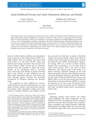
Table 2 shows that additional income in the prenatal to age 5 period for the lowest-income children
is associated with significantly greater adult earnings and work hours, and less food stamp receipt.
To ensure that our spline models fit the earnings
and work hours data reasonably well, we estimated
models with early income represented with a set of
dummy variables, and controls for later period
incomes (ages 6 through 10 and ages 11 through
15). As shown in Figures 1 and 2, which include
95% confidence bands, the income range in which
income responses flattened out was roughly
between $20,000 and $30,000, thus supporting our
use of a knot at $25,000.
We can illustrate the nature of the income effects
of early-childhood income using the natural log
earnings regression. The ‘‘0.52’’ coefficient means
that, adjusting for income later in childhood and
the other control variables listed in Table 2, an
additional $10,000 per year of family income
between the prenatal year and the child’s fifth
birthday is associated with an increase in the natural logarithm of adult earnings of 0.52—or 68.2%
(e52 = 1.682). In contrast, increments to early-childhood income for higher-income children (i.e.,
annual average family incomes above $25,000) are
associated with an insignificant 0.05 increment in
log earnings. The p value (p < .05) reported in the
‘‘different slopes’’ column indicates that the slope
for those with incomes less than $25,000 per year in
early childhood is significantly different from the
slope for those with incomes greater than $25,000
in the same period. Increments to incomes in middle childhood and adolescence are estimated to
have nonsignificant impacts on log earnings, even
among low-income children. The final row of
Table 2 indicates that the three coefficients on the
< $25,000 spline slopes across the childhood stages
are significantly different from one another at the
p = .08 level.
Results for work hours are broadly similar to
those for earnings—a highly significant estimated
impact of early childhood but not later childhood
income. In this case, a $10,000 annual increase in
the prenatal to age 5 income of low-income families
is associated with more than 500 additional work
hours per year after age 25. Tobit spline regressions
for food stamps for the entire sample suggest that
increases in income in all childhood periods for the
lowest income children are associated with statistically significant reductions in food stamps. Both the
coefficients on food stamps and welfare proved

10. <
>
<
>
<
>
0.10 (0.10)
)0.12 (0.35)
0.53** (0.07)
)0.02 (0.12)
)0.09 (0.07)
0.00 (0.01)
0.02 (0.02)
0.19* (0.08)
)0.01 (0.02)
0.02 (0.02)
)0.03 (0.04)
0.00 (0.03)
)0.04 (0.11)
0.04 (.12)
0.04 (0.03)
Yes
.24
1,016
.08
.29
1,254
.04
p < .10
p < .01
ns
ns
p < .05
0.52* (0.21)
0.05** (0.02)
0.14 (0.14)
0.01 (0.02)
0.04 (0.12)
0.00 (0.01)
ns
0.76** (0.24)
0.68 (0.57)
)0.45** (0.13)
0.63** (0.22)
)0.16 (0.18)
0.04* (0.02)
)0.09 (0.06)
0.32* (0.15)
0.10* (0.04)
0.10** (0.03)
)0.09 (0.08)
0.14* (0.06)
)0.32 (0.23)
0.26 (0.22)
0.16** (0.05)
Yes
$25K 0.19 (0.33)
$25K 0.03 (0.04)
$25K 0.65** (0.25)
$25K )0.06 (0.04)
$25K )0.31 (0.20)
$25K 0.09** (0.03)
Different
slopes
Different
slopes
ln Earnings
(ages 25–37)
.24
1,042
.01
)79.44
(82.40)
)255.48 (219.46)
566.54** (48.12)
47.66
(80.15)
)32.16
(57.65)
1.46
(6.17)
)9.49
(21.89)
102.51 (58.86)
)8.04
(17.10)
)6.71
(10.84)
12.19
(26.51)
15.16
(23.21)
)6.66
(81.76)
)78.53
(86.30)
10.86
(19.70)
Yes
.03
1,198
.73
368.48** (78.44)
213.80 (134.61)
)191.19** (52.78)
76.63
(86.08)
)35.53
(58.49)
)8.98
(5.85)
20.23
(16.95)
)79.03
(61.51)
19.06
(15.02)
)24.49* (11.75)
39.42
(29.48)
)72.21** (24.41)
25.80
(80.99)
98.89
(89.62)
)37.43 (19.95)
Yes
p < .10
506.74** (135.39) p < .001 )279.5* (142.08)
20.60*
(9.78)
)4.34
(14.17)
)60.82 (109.42)
ns
)380.30** (128.37)
1.28
(8.36)
3.91
(11.89)
74.18
(83.33)
ns
)221.71* (101.53)
)0.92
(7.56)
)6.07
(9.92)
p < .05
p < .01
Different
slopes
Annual food
stamp (ages 25–37)
Different
slopes
Annual hours
worked (ages 25–37)
.04
601
.38
964.63* (155.28)
)312.59 (378.53)
—
)146.97 (172.44)
)511.95** (116.70)
)17.56
(12.87)
14.67
(35.90)
)246.83* (118.84)
)33.86
(27.70)
17.37
(24.45)
)12.67
(54.20)
)187.05** (47.26)
)9.63 (162.68)
227.59 (172.27)
24.36
(42.44)
Yes
)157.28 (267.04)
12.02
(24.60)
419.06 (233.44)
)25.91
(27.44)
172.35 (202.78)
)37.73
(23.59)
—
ns
p < .10
ns
Different
slopes
Annual AFDC ⁄ TANF
Females only (ages 25–37)
Note. Sample consists of Panel Study of Income Dynamics children born between 1968 and 1975. Incomes are in 2005 dollars and childhood incomes are scaled in $10,000. Data in
the ‘‘different slopes’’ column show p levels of test of equality of within-period < $25K and > $25K slopes. The coefficients and standard errors for the schooling, earnings, and
hours are from ordinary least squares (OLS) analysis, and the coefficients and standard errors for food stamps and Aid to Families with Dependent Children ⁄ Temporary
Assistance to Needy Families (AFDC ⁄ TANF) are from Tobit analysis. The AFDC ⁄ TANF analysis is only for females. Regressions are weighted and OLS analysis standard errors
are corrected for multiple children born in the same household.
p < .10. *p < .05. **p < .01.
Average annual
income (prenatal to age 5)
Average annual
income (ages 6–10)
Average annual
income (ages 11–15)
Other variables
Black
Other minority
Child is male
Child born into intact family
Child born in South
Age of mother at time of birth
Number of siblings
Child is firstborn
HH head test score (1972)
HH head schooling
Observed ‘‘dirty’’ home
Parental expectations
Challenge versus affiliation
Personal control
Risk avoidance
Birth year dummies?
Regression statistics
R2
Number of observations
p from test of equality of
three < $25K spline segments
Childhood income (in $10,000)
Years of completed
schooling
Table 2
Ordinary Least Squares Spline Regression Models of Childhood Income and Completed Schooling, Adult Earnings and Annual Work Hours, and Tobit Spline Models of Childhood Income and Program Participation
Early-Childhood Poverty
315

11. <
>
<
>
<
>
$25K
$25K
$25K
$25K
$25K
$25K
.14
1,137
.96
0.025 (0.025)
)0.009 (0.042)
0.014 (0.014)
0.014 (0.016)
0.007 (0.015)
0.001 (0.001)
)0.006 (0.004)
)0.024 (0.014)
0.000 (0.004)
)0.004 (0.002)
0.000 (0.007)
)0.007 (0.006)
0.023 (0.023)
0.002 (0.023)
)0.004 (0.005)
Yes
)0.009 (0.027)
0.003 (0.003)
)0.008 (0.027)
0.007 (0.004)
0.001 (0.028)
)0.017** (0.003)
ns
ns
ns
Different
slopes
(0.021)
(0.003)
(0.016)
(0.002)
(0.021)
(0.002)
.42
.22
529
)0.024* (0.014)
—
)0.024 (0.014)
)0.009 (0.021)
0.011 (0.013)
0.000 (0.001)
0.002 (0.003)
0.003 (0.010)
)0.007* (0.003)
)0.001 (0.002)
)0.004 (0.005)
)0.002 (0.005)
0.027 (0.020)
)0.011 (0.015)
0.003 (0.002)
Yes
0.011
)0.002
0.013
0.006*
)0.026
)0.006*
ns
ns
ns
Different
slopes
High distress (2003)
(2.45)
(0.16)
(1.51)
(0.09)
(1.41)
(0.09)
.11
875
.36
0.36 (0.83)
)0.77 (0.87)
1.73** (0.47)
)0.09 (0.94)
)0.20 (0.55)
0.02 (0.06)
0.13 (0.18)
0.65 (0.49)
)0.17 (0.14)
)0.16 (0.11)
0.59* (0.29)
)0.16 (0.26)
)0.41 (0.71)
0.10 (0.86)
)0.12 (0.19)
Yes
)3.51
0.04
0.77
)0.12
0.34
0.06
ns
ns
ns
Different
slopes
BMI (2005)
(0.113)
(0.014)
(0.107)
(0.010)
(0.097)
(0.008)
.39
.10
875
)0.039 (0.089)
)0.014 (0.153)
0.278** (0.043)
0.059 (0.093)
)0.062 (0.053)
)0.009 (0.006)
0.015 (0.018)
0.020 (0.052)
)0.023 (0.013)
)0.018 (0.010)
0.038 (0.028)
0.004 (0.023)
)0.012 (0.078)
)0.014 (0.081)
)0.017 (0.017)
Yes
0.028
0.013
)0.130
)0.020*
0.128
0.010
ns
ns
ns
Different
slopes
Overweight
(BMI > 25 in 2005)
Note. Sample consists of Panel Study of Income Dynamics children born between 1968 and 1975. Incomes are in 2005 dollars, and childhood incomes are scaled in $10,000. Data in
the ‘‘different slopes’’ column show p levels of test of equality of within-period < $25K and > $25K slopes. Marginal effects from logistic spline regressions presented for poor
health, high distress, and overweight. Poor health regression includes year-of-report dummy variables. Regressions are weighted and standard errors are corrected for multiple
children born in the same household. Logistic regression models present marginal effects and standard errors. Marginal effects are interpreted as probabilities and are computed
using the MFX command in STATA. BMI = body mass index.
p < .10. *p < .05. **p < .01.
Average annual
income (prenatal to age 5)
Average annual
income (ages 6–10)
Average annual
income (ages 11–15)
Other variables
Black
Other minority
Child is male
Child born into intact family
Child born in South
Age of mother at time of birth
Number of siblings
Child is firstborn
Household head test score (1972)
Household head schooling (1972)
Observed ‘‘dirty’’ home
Parental expectations
Challenge versus affiliation
Personal control
Risk avoidance
Birth year dummies?
Regression statistics
R2 (or pseudo)
Number of observations
p level of test of equality for
the three < $25K spline segments
Childhood income (in $10,000)
Poor health
Table 3
Logistic Spline Regression Models of Childhood Income and Poor Health, High Distress, and Overweight; Ordinary Least Squares Spline Regression Model of Childhood Income and Body Mass
Index
316
Duncan, Ziol-Guest, and Kalil

12. <
>
<
>
<
>
$25K
$25K
$25K
$25K
$25K
$25K
(0.055)
(0.011)
(0.061)
(0.009)
(0.050)
(0.007)
.90
.13
744
)0.052 (0.032)
)0.039 (.079)
)0.085 (0.054)
)0.020 (0.033)
)0.005 (0.004)
0.020* (0.010)
0.015 (0.036)
)0.008 (0.008)
0.002 (0.07)
)0.042* (0.021)
0.030* (0.015)
0.076 (0.050)
0.015 (0.045)
)0.036** (0.011)
Yes
0.013
)0.018
)0.024
0.016
)0.015
)0.013
ns
ns
.87
.18
744
)0.013 (0.017)
)0.012 (0.044)
)0.041 (0.031)
)0.015 (0.018)
)0.005* (0.002)
0.004 (0.007)
)0.014 (0.016)
)0.002 (0.004)
0.004 (0.004)
)0.015 (0.010)
)0.003 (0.018)
0.020 (0.023)
)0.002 (0.023)
)0.016 (0.007)
Yes
ns
ns
ns
ns
0.017 (0.028)
0.001 (0.06)
)0.004 (0.027)
)0.001 (0.004)
0.000 (0.021)
)0.009** (0.004)
Different
slopes
Different
slopes
Ever jailed (males)
.41
.29
778
0.135** (0.049)
0.052 (0.110)
)0.012 (0.034)
)0.048* (0.024)
)0.007* (0.003)
0.020* (0.009)
)0.006 (0.029)
)0.009 (0.006)
)0.009 (0.005)
)0.015 (0.013)
)0.020 (0.011)
0.044 (0.037)
)0.093* (0.046)
0.004 (0.009)
Yes
0.049 (0.046)
0.002 (0.012)
0.013 (0.045)
0.000 (0.009)
)0.035 (0.042)
)0.021** (0.008)
ns
ns
ns
Different
slopes
Nonmarital birth (females)
Note. Sample consists of Panel Study of Income Dynamics children born between 1968 and 1975. Incomes are in 2005 dollars. Childhood incomes are scaled in $10,000. Data in the
‘‘different slopes’’ column show p levels of test of equality of within-period < $25K and > $25K slopes. Regressions are weighted and standard errors are corrected for multiple
children born in the same household. Logistic regression models present marginal effects and standard errors. Marginal effects are interpreted as probabilities and are computed
using the MFX command in STATA.
p < .10. *p < .05. **p < .01.
Average annual
income (prenatal to age 5)
Average annual
income (ages 6–10)
Average annual
income (ages 11–15)
Other variables
Black
Other minority
Child born into intact family
Child born in South
Age of mother at time of birth
Number of siblings
Child is firstborn
Household head test score (1972)
Household head schooling
Observed ‘‘dirty’’ home
Parental expectations
Challenge versus affiliation
Personal control
Risk avoidance
Birth year dummies?
Regression statistics
Pseudo R2
Number of observations
p level of test of equality for
the three < $25K spline segments
Childhood income (in $10,000)
Ever arrested (males)
Table 4
Logistic Spline Regression Models of Childhood Income and Arrests, Jailed, and Nonmarital Births
Early-Childhood Poverty
317

13. 318
Duncan, Ziol-Guest, and Kalil
Figure 1. Adult ln earnings by early-childhood income, with 95% confidence intervals.
Figure 2. Adult work hours by early-childhood income, with 95% confidence intervals.
somewhat sensitive to outliers, resulting in a decision to truncate both dependent variables at the
99th percentiles of their respective distributions—$4,913 in the case of annual food stamp
receipt and $2,954 in the case of annual AFDC ⁄
TANF receipt. Additionally, when separate food
stamp models for males and females were conducted, we found a much larger and statistically
different effect of early poverty for females than for
males. The respective coefficients and standard
errors for females were )$483 (268) and for males
were )$260 (125). The female coefficient has a
p = .06; the male coefficient has a p = .04.
The coefficient on early income in the schooling
regression is 0.19 years, which is not statistically
significant at conventional levels (p = .569). The
lack of a significant regression-adjusted association
between early income and schooling is at odds with
results presented in Duncan et al. (1998). The present analysis includes three different birth cohorts
than Duncan et al. and the early income–schooling
relation appears somewhat weaker for the new
cohorts. A more interesting difference is that Duncan et al. assessed completed schooling by age
20—a kind of ‘‘on time’’ schooling measure. We
tested several alternative schooling specifications,
including completed schooling by age 21, on-time
high school graduation (by age 18 or 19), had
dropped out of high school as of age 21, and had
attended some college as of age 21. In the case of

14. Early-Childhood Poverty
completed schooling by age 21, we found that the
coefficient on early income was 0.338 and statistically
significant (p < .05). Further, when examining a
specification that includes four time periods (prenatal through ages 2, ages 3 through 5, ages 6 through
10, and ages 11 through 15), the coefficient on age 3
through 5 was significant both for completed
schooling by age 21 (0.399) and for on-time high
school graduation (marginal probability effect from
a logistic regression of 0.182). So it appears that
early income may matter more for the on-time completion of schooling by the end of adolescent than
for the sporadic increases in schooling that often
occur later.
Results for the control variables in the completed
schooling regression mirror past research, with
Black people (adjusted for socioeconomic status
and other controls), females, children born first,
into intact or smaller families, or born to older
mothers, more educated parents, greater household
head expectations at birth or greater household
head risk avoidance, obtaining more schooling.
Few of these controls have persistently significant
coefficients across all of the attainment-related outcomes in Table 2.
The marginal (probability change) effects from
logistic spline models for poor health, high distress
and overweight, and OLS results for BMI are
shown in Table 3 and show scattered income effects
in middle childhood and adolescence, but not early
childhood. In no case are increments to low income
in later childhood stages estimated to have a statistically significant impact on any of the health outcomes.
Table 4 presents marginal effects for the behavioral outcomes for men (arrests and jail) and
women (nonmarital childbearing). Here again, the
early-childhood income segments are not statistically significant in any of these models. As in the
case of the health, increments to low income in
middle childhood and adolescence are never estimated to have a statistically significant impact on
any of the behavioral outcomes.
Extensions to Main Analysis
We explored the robustness of our results in various ways, first by testing for sex and race interactions. We found no statistically significant
interactions by sex. For the race interactions, the
incarceration of Black men appeared to be significantly less sensitive to increments in early-childhood income than the incarceration of White men.
Specifically, the coefficient, expressed as a marginal
319
effect on the probability of occurrence, on White
incarceration was 0.38 (SE = 0.16) and the Black difference was )0.36 (SE = 0.16).
In averaging early-childhood income over the 7year interval between the prenatal year and fifth
birthday, there is a danger that we are missing a
narrower sensitive period of income effects. In
Table 5, we present results from regressions that
are identical to those in Tables 2–4 except that the
prenatal to age 5 period is further divided into two
segments—the prenatal and birth years and ages 1
through 5. A comparison of coefficients shows that
point estimates of income effects for four of the five
attainment-related outcomes are all larger when
income is measured between ages 1 and 5 than earlier, although only in the case of completed schooling is the difference statistically significant.
The opposite is true of body mass—very early
income appears to matter more than income after
the birth year, a result explored in some depth in
Ziol-Guest, Duncan, and Kalil (2009). This finding
of the particular importance of income during the
prenatal and birth years for adult BMI may support
the ‘‘fetal origins’’ hypothesis.
A more technical concern involving the income
measure is that it is pretax total family income. An
after-tax measure might better capture a family’s
spending opportunities and constraints. We re-estimated our models using childhood income measures from which PSID-calculated federal income
taxes had been subtracted. The results proved
somewhat sensitive to outliers but were generally
quite similar to those shown earlier.
Table 6 explores the robustness of the prenatalto-age-5 low-income coefficients in two additional
models. The coefficients and standard errors in the
first column are identical to those presented in
Tables 2–4. In the second column, we retain all of
the control variables, but in this case maternal earnings have been subtracted from all three stagespecific income variables. This helps to address the
problem that mother’s earnings are a component of
childhood income. Mothers’ labor supply decisions
have implications for the amount of time mothers
can spend with their children and may be affected
by how successful the child’s development is
viewed by the family. For earnings and annual
work hours for which early income effects were statistically significant in Table 2, the new income
coefficients are smaller but retain statistical significance.
Stage-specific income results presented in
Carneiro and Heckman (2003, p. 120) employ a
somewhat different specification than ours in which

15. 320
Duncan, Ziol-Guest, and Kalil
Table 5
Coefficients and Standard Errors From Models in Which Prenatal to Age 5 Income Is Divided Into (a) Prenatal and Birth Years and (b) Ages 1–5
Coefficients and standard errors on low-income < $25K
spline segment
Average annual income,
prenatal to birth (< 25K)
Average annual income,
ages 1–5 (< 25K)
Different
slopes
)0.46
(0.30)
0.17
(0.18)
188.70 (131.00)
)276.59* (137.75)
)100.68 (22.58)
0.01
(0.03)
0.01
(0.04)
)2.16* (1.08)
)0.11
(0.10)
0.02
(0.06)
0.02
(0.03)
0.00
(0.05)
0.63 (0.38)
0.32
(0.21)
317.60* (129.23)
)160.59 (133.63)
)425.68* (220.25)
)0.03
(0.03)
0.00
(0.02)
)1.45
(2.11)
0.10
(0.11)
)0.03
(0.06)
)0.01
(0.03)
0.08 (0.04)
p < .05
ns
ns
ns
ns
ns
ns
ns
ns
ns
ns
ns
Completed schooling
ln Earnings
Annual hours worked
Annual food stamp receipt
Annual AFDC ⁄ TANF receipt (females)
Poor health
High distress
Body mass index
Overweight
Arrested (males)
Incarcerated (males)
Nonmarital childbearing (females)
Note. Sample consists of Panel Study of Income Dynamics children born between 1968 and 1975. Incomes are in 2005 dollars and
childhood incomes are scaled in $10,000. Coefficient and standard errors from regressions that contain all control variables and four
spline segments: prenatal through birth year, ages 1 through 5, ages 6 through 10, and ages 11 through 15. Different slopes indicates
whether the low-income segment between prenatal and birth is significantly different from between ages 1 and 5. Ordinary least
squares coefficients shown for completed schooling, earnings, annual hours worked, and body mass index; Tobit coefficients shown for
food stamps and Aid to Families with Dependent Children ⁄ Temporary Assistance to Needy Families (AFDC ⁄ TANF); and marginal
effects shown for the dichotomous outcomes. Marginal effects are interpreted as probabilities and are computed using the MFX
command in STATA.
p < .10. *p < .05.
Table 6
Coefficients and Standard Errors on Average Annual Income Prenatal to Age 5 < 25K for Various Model Specifications
Coefficients and standard error on
low-income (< $25K) spline segment
Controls for permanent
(prenatal to age 15) income
Basic
regression
Completed schooling
ln Earnings
Annual hours worked
Annual food stamp receipt
Annual AFDC ⁄ TANF receipt
(females only)
Poor health
High distress
Body mass index
Overweight
Arrested
Incarcerated
Nonmarital childbearing
Exclude maternal
earnings from all
childhood income
measures
Coefficient on
low-income
permanent income
spline segment
Coefficient on
low-income
prenatal-to-age-5
spline segment
0.19
(0.33)
0.52*
(0.21)
506.74** (135.39)
)303.14* (152.09)
)419.18 (264.28)
)0.25
(0.22)
0.36** (0.11)
220.65** (78.04)
)102.12
(87.98)
)90.34 (162.55)
0.81*
(0.36)
0.33
(0.20)
63.55 (124.30)
)1152.47** (187.07)
943.17** (340.79)
)0.11
(0.37)
0.39
(0.22)
446.56** (146.96)
149.98 (195.37)
)570.57 (387.58)
)0.01
0.01
)3.51
0.03
0.01
0.02
0.05
(0.03)
(0.012)
(2.45)
(0.11)
(0.05)
(0.03)
(0.05)
0.012
0.001
)1.57
0.038
)0.004
0.014
0.038
(0.015)
(0.009)
(1.03)
(0.063)
(0.041)
(0.020)
(0.029)
0.014
)0.031
2.34
0.058
)0.008
0.012
)0.082
(0.031)
(0.030)
(1.47)
(0.138)
(0.080)
(0.031)
(0.044)
)0.032
0.039
)4.62
)0.060
)0.006
0.006
0.107
(0.0338)
(0.043)
(2.62)
(0.140)
(0.071)
(0.029)
(0.058)
Note. Marginal effects reported for the dichotomous outcomes. AFDC ⁄ TANF = Aid to Families with Dependent Children ⁄ Temporary
Assistance to Needy Families.
p < .10. *p < .05. **p < .01.

16. Early-Childhood Poverty
childhood income is characterized by permanent
(i.e., all-childhood-year average) income and just
the early-childhood component. In this case, the
coefficient on the early income component shows
the coefficient difference from permanent income. As
shown in the last pair of columns in Table 6, we
find that early income is significantly more predictive of earnings and work hours than is permanent
childhood income.
One concern in these types of analyses is omitted
variable bias, and one approach to deal with this
concern is to conduct sibling difference models that
capitalize on within-family variation (Johnson &
Schoeni, 2007). We tested these models for the earnings and annual work hours regressions. Because of
small sample sizes, precision is a problem. For
earnings, the coefficient (standard error) on the
lower income spline segment was 0.30 (1.08) compared to 0.52 (0.21) in the full sample and the
higher income spline was 0.07 (0.09) compared to
0.14 (0.14). For annual work hours, the coefficient
and standard error on the lower income spline was
1047 (969) compared to 507 (135) in the full analysis; whereas the higher income early-childhood
coefficient in the sibling fixed effects model was )8
(78) compared to 20 (10) in the analysis presented
in Table 2.
Given the interesting results for the log earnings
models, we sought to explore mediational pathways by sequentially introducing the sets of predictors listed in the columns of Table 7. Controls for
childhood maternal work hours and family compo-
321
sition had little impact on the key early-income
coefficient. Because controls for work hours and
family structure are not so much mediators as additional childhood controls that might be biasing our
income estimates, we have not included them in
our basic models owing to their potential endogeneity. Completed schooling accounts for very little
of the income effect, which is hardly surprising
given the weak links between early income and
schooling (see Appendix A). The same explanation
probably underlies the lack of a mediational role
for the behavior and health measures. On the other
hand, the inclusion of adult work hours reduces
the early-income coefficient by 80%, which suggests
that much of the earnings impact of early-childhood income operates through annual work hours
rather than wage rate.
The importance of work hours in the link
between early-childhood income and annual adult
earnings suggests that childhood income should
have a relatively small effect on hourly earnings in
adulthood. When we used average hourly earnings
after age 25 as a dependent variable in our standard
full-control regression model, the coefficient on
early-childhood income was small and statistically
insignificant. We investigated the work hours effects
further by estimating whether early-childhood
income appeared to operate by reducing unemployment or time out of the labor force altogether as
opposed to full versus part-time work. For both
men and women, the income effects were the strongest for full versus less-than-full time work.
Table 7
Accounting for the Effects of Prenatal to Age 5 Average Annual Income on Log Earnings
Coefficients and standard error on low-income < $25K spline segment in
ln earnings regression
Basic
model
Add
childhood
conditions
Add
schooling
Add
adult
behavior
Add
adult
health
Add
adult
work hours
Average annual income < $25K (prenatal to age 5)
0.52* (0.21) 0.64** (0.22) 0.60** (0.21) 0.64** (0.21) 0.59** (0.20) 0.10 (0.14)
Average annual income (ages 6–10 and 11–15)
incl.
incl.
incl.
incl.
incl.
incl.
Other background controls
incl.
incl.
incl.
incl.
incl.
incl.
Prenatal to age 15 maternal work hours and family structure
incl.
incl.
incl.
incl.
incl.
Completed schooling
incl.
incl.
incl.
incl.
Arrests, jail, and out-of-wedlock childbearing
incl.
incl.
incl.
Adult health
incl.
incl.
Work hours
incl.
Regression statistics
R2
.24
.25
.33
.34
.35
.61
Number of observations
1,016
1,016
1,016
1,016
1,016
1,016
*p < .05. **p < .01.

17. 322
Duncan, Ziol-Guest, and Kalil
Conclusion
Our exploration of the role of economic deprivation early in childhood produced surprisingly
strong associations in the case of two important
adult attainments—earnings and work hours. These
results complement those reported in Duncan and
Brooks-Gunn (1997), who found stronger correlations between early-childhood income and childhood achievement than between early income and
either childhood behavior or health.
One way of assessing the policy significance of our
coefficients is to express our results in income increments that have been associated with past policy
changes. With the EITC transferring as much as
$4,800 to working families, we used $3,000 as a possible increment. The coefficients imply that a $3,000
annual increase in income between a child’s prenatal
year and fifth birthday is associated with 19% higher
earnings and a 135-hr increase in work hours. Moreover, most of the childhood-income effects on earnings appear to be accounted for by differences in
annual work hours, suggesting that the results for
work hours are particularly important to understand.
Apart from studies looking at adult ‘‘idleness’’
(Haveman & Wolfe, 1994), there is little work on the
childhood determinants of full-time work.
One important policy issue is the persistence of
these effects across adulthood. A supplemental earnings regression that included an interaction between
early-childhood income and age at which adult earnings were measured (not shown in the tables) indicated that the 19% proportionate impact of earlychildhood poverty did not change over the ages for
which we are able to track the sample (ages 25–37), so
we can safely assume that the childhood income
impact persists for at least that 13-year period.
We end with the usual cautions regarding the
causal interpretation of our income ‘‘effects.’’
Among the many approaches to estimating the causal impacts of childhood income on adult outcomes, ours is more sophisticated than some but
less sophisticated than others. We are the first
study to link high-quality income data across the
entire childhood period with adult outcomes measured as late as age 37.
The incomes we observe are determined, in part,
by the actions of parents and other family members, which leave our analyses open to omitted-variable bias. Our list of variables controlling for
conditions at the time of birth is extensive and
ought to reduce a good deal of potential bias. More
important, and unusual for studies such as ours, is
that our estimates of the impacts of early-childhood
income control for income in middle childhood and
adolescence. As such, factors such as genetic influences are as likely to affect later and early-childhood income, and thus are controlled, in some
degree, by our inclusion of income in other childhood stages. Nevertheless, the possibility of lingering omitted-variable bias remains.
References
Barker, D. (1998). Mothers, babies, and health in later life.
Edinburgh, UK: Churchill Livingstone.
Barker, D. J. P., Eriksson, J. G., Forsen, T., & Osmond, C.
(2002). Fetal origins of adult disease: Strength of effects
and biological basis. International Journal of Epidemiology, 31, 1235–1239.
´
Barker, D. J. P., Osmond, C., Forsen, T. J., Kajantie, E., &
Eriksson, J. (2005). Trajectories of growth among children who have coronary events as adults. New England
Journal of Medicine, 353, 1802–1809.
Blau, D. (1999). The effect of income on child achievement. Review of Economics and Statistics, 81, 261–276.
Bronfenbrenner, U., & Morris, P. (1998). The ecology of
developmental processes. In W. Damon (Series Ed.) &
R. M. Lerner (Vol. Ed.), Handbook of child psychology:
Vol. 1. Theoretical models of human development (5th ed.,
pp. 993–1028). New York: Wiley.
Carneiro, P., & Heckman, J. (2003) Human capital policy.
In J. Heckman & A. Krueger (Eds.), Inequality in America: What role for human capital policies? (pp. 77–239).
Cambridge, MA: MIT Press.
Centers for Disease Control and Prevention. (2003).
Healthy weight, overweight, and obesity among US adults.
Available at www.cdc.gov/nchs/data/nhanes/databriefs/
adultweight.pdf. Accessed on November 1, 2007.
Cunha, F., Heckman, J. J., Lochner, L., & Masterov, D.
(2005). Interpreting the evidence on life cycle skill formation. In E. Hanushek & F. Welch (Eds.), Handbook of
the economics of education (pp. 697–812). Amsterdam:
North Holland.
Dahl, G., & Lochner, L. (2005). The impact of family income on
child achievement (NBER Working Paper No. 11279). Cambridge, MA: National Bureau of Economic Research.
Danese, A., Pariante, C., Caspi, A., Taylor, A., & Poulton,
R. (2007). Childhood maltreatment predicts adult
inflammation in a life-course study. Proceedings of the
National Academy of Sciences of the United States of America, 104, 1319–1324.
Duncan, G. J. (1988). The volatility of family income over the
life course. In P. B. Baltes, D. L. Featherman, & R. M. Lerner (Eds.), Life-span development and behavior (Vol. 9, pp.
317–358). Hillsdale, NJ: Erlbaum.
Duncan, G. J., & Dunifon, R. (1988). Soft skills and longrun labor market success. In S. W. Polacheck & J. Robst
(Eds.), Research in labor economics (Vol. 17, pp. 123–150).
London: JAI Press.

18. Early-Childhood Poverty
323
Proceedings of the National Academy of Sciences of the United States of America, 103, 10155–10162.
Mayer, S. (1997). What money can’t buy: The effect of parental income on children’s outcomes. Cambridge, MA: Harvard University Press.
Menard, S. (2004). Six approaches to calculating standardized logistic regression coefficients. American Statistician, 58, 218–223.
Poulton, R., & Caspi, A. (2005). Commentary: How does
socioeconomic disadvantage during childhood damage
health in adulthood? Testing psychosocial pathways.
International Journal of Epidemiology, 34, 344–345.
Rowe, D., & Rodgers, J. (1997). Poverty and behavior: Are
environmental measures nature and nurture? Developmental Review, 17, 358. 375.
Sapolsky, R. (2004). Mothering style and methylation.
Nature Neuroscience, 7, 791–792.
Shonkoff, J., & Phillips, D. (Eds.). (2000). From neurons to
neighborhoods: The science of early childhood development,
Washington, DC: National Academy Press.
Stunkard, A., Faith, M., & Allison, K. (2003). Depression
and obesity. Biological Psychology, 54, 330–337.
U.S. Census Bureau. (2008). Retrieved February 1, 2008,
from http://www.census.gov/hhes/www/poverty/
poverty.html
Waddington, C. H. (1957). The strategy of genes. Boston:
Allen & Unwin.
Waters, E., & Sroufe, L. A. (1983). Social competence as a
developmental construct. Development and Psychopathology, 3, 79–97.
Yeung, W. J., Linver, M., & Brooks-Gunn, J. (2002). How
money matters for young children’s development:
Parental investment and family processes. Child Development, 73, 1861–1879.
Ziol-Guest, K. M., Duncan, G. J., & Kalil, A. (2009). Early
childhood poverty and adult body mass index. American Journal of Public Health, 99, 527–532.
Duncan, G. J., & Brooks-Gunn, J., (Eds.). (1997). Consequences of growing up poor. New York: Russell Sage
Foundation.
Duncan, G. J., Brooks-Gunn, J., Yeung, W., & Smith, J.
(1998). How much does childhood poverty affect the
life chances of children? American Sociological Review,
63, 406–423.
Dunifon, R., Duncan, G. J., & Brooks-Gunn, J. (2001). As
ye sweep, so shall ye reap. American Economic Review:
Papers and Proceedings, 91, 150–154.
Fox, N. (1994). The development of emotion regulation:
Biological and behavioral considerations. Monographs of
the Society for Research in Child Development, 59(2 ⁄ 3),
152–166.
Frongillo, E. (2003). Understanding obesity and program
participation in the context of poverty and food insecurity. Journal of Nutrition, 133, 2117–2118.
Godfrey, K. M., & Barker, D. J. P. (2000). Fetal nutrition
and adult disease. American Journal of Clinical Nutrition,
71, 1344S–1352S.
Haveman, R., & Wolfe, B. (1994). Succeeding generations.
New York: Russell Sage Foundation.
Hertzman, C. (1999). The biological embedding of
early experiences and its effects on health in adulthood. Annals of the New York Academy of Sciences, 896,
85–95.
Holzer, H., Schanzenbach, D., Duncan, G., & Ludwig, J.
(2007) The economic costs of poverty in the United States:
Subsequent effects of children growing up poor. Washington, DC: Center for American Progress.
Johnson, R., & Schoeni, R. (2007). The influence of early-life
events on human capital, health status and labor market outcomes over the life course (Working paper). Berkeley, CA:
Goldman School of Public Policy.
Knudsen, E., Heckman, J., Cameron, J., & Shonkoff, J.
(2006). Economic, neurobiological, and behavioral
perspectives on building America’s future workforce.
Appendix A
Weighted Descriptive Statistics of Adult Outcomes by Prenatal to Age 5 Poverty
Total sample
Income below the
official poverty line
(A)
SD
M or %
SD
Income more than
twice the poverty
line (C)
M or %
SD
Significant
difference
M or %
Completed schooling
Unweighted n
Earnings ($10,000)
Unweighted n
Annual work hours
Unweighted n
Food stamps
M or %
Income
between 1 and
2 times the
poverty line (B)
SD
13.39
1,254
34.56
1,042
1,892.46
1,042
213.75
2.14
11.83
1.83
12.70
2.02
13.96
2.01
A < B,C; B < C
30.93
17.86
16.00
26.79
21.17
39.67
33.96
A < B,C; B < C
699.30
1,512.37
750.25
1,839.12
778.77
1,963.08
641.63
A < B,C; B < C
730.30
896.28
1,453.87
337.28
902.25
70.09
337.43
A > B,C; B > C

19. 324
Duncan, Ziol-Guest, and Kalil
Appendix A
Continued
Total sample
Income more
than twice the
poverty line (C)
SD
1,157
158.72
574
0.08
1,167
0.04
667
27.46
875
0.61
875
0.16
757
0.09
757
0.20
778
M or %
SD
M or %
SD
M or %
SD
Significant
difference
750.60
M or %
Unweighted n
AFDC ⁄ TANF (women only)
Unweighted n
Poor health
Unweighted n
High distress
Unweighted n
Body mass index
Unweighted n
Overweight
Unweighted n
Arrested (men only)
Unweighted n
Incarcerated (men only)
Unweighted n
Nonmarital birth (women only)
Unweighted n
Income between 1
and 2 times the
poverty line (B)
Income below
the official
poverty line (A)
285.63
804.07
380.61
1,231.28
46.14
344.06
A,B > C
—
0.13
—
0.13
—
0.05
—
A,B > C
—
0.10
—
0.04
—
0.04
—
ns
5.87
30.63
7.27
28.05
6.70
26.86
5.22
A > B,C; B > C
—
0.79
—
0.61
—
0.59
—
A > B,C
—
0.26
—
0.21
—
0.13
—
A,B > C
—
0.10
—
0.12
—
0.07
—
B>C
—
0.50
—
0.28
—
0.09
—
A > B,C; B > C
Note. In the ‘‘significant difference’’ column, A < B signifies that the mean of those less than the poverty line is statistically significantly
smaller than those between 1 and 2 times the poverty line at p < .05 (two-tailed). A > B signifies that the mean of those less than the poverty line is statistically significantly larger than those between 1 and 2 times the poverty line at p < .05 (two-tailed). Earnings, food stamp
value, and Aid to Families with Dependent Children ⁄ Temporary Assistance to Needy Families (AFDC ⁄ TANF) value in 2005 dollars.
Appendix B
Weighted Descriptive Statistics of Control Variables by Prenatal to Age 5 Poverty
Total sample
Income below the
official poverty line
(A)
Income between
1 and 2 times the
poverty line (B)
Income more than
twice the poverty
line (C)
M or %
Prenatal to age 5, average
annual income (2005$)
Ages 6–10, average
annual income (2005$)
Ages 11–15, average
annual income (2005$)
White
Black
Other minority
Male
Born into intact family
Born in the South
Age of mother at birth
Number of siblings
SD
M or %
SD
M or %
SD
M or %
SD
Significant
difference
47,842.48
28,340.64
21,400.11
9,714.14
36,024.01
12,242.22
65,442.38
28,776.41
A < B,C; B < C
54,226.12
39,012.65
23,112.91
16,197.13
41,956.34
23,148.25
73,881.51
42,250.67
A < B,C; B < C
59,067.89
45,369.20
24,743.16
20,140.42
44,137.52
27,222.75
81,649.59
49,337.59
A < B,C; B < C
0.77
0.19
0.04
0.53
0.84
0.32
24.84
2.21
—
—
—
—
—
—
5.76
1.79
0.38
0.58
0.04
0.52
0.44
0.51
24.04
4.00
—
—
—
—
—
—
7.23
3.07
0.70
0.26
0.04
0.52
0.78
0.39
24.13
2.56
—
—
—
—
—
—
6.29
1.73
0.88
0.09
0.04
0.54
0.94
0.26
25.29
1.74
—
—
—
—
—
—
5.15
1.16
A < B,C; B <
A > B,C; B >
ns
ns
A < B,C; B <
A > B,C; B >
A,B < C
A > B,C; B >
C
C
C
C
C

20. Early-Childhood Poverty
325
Appendix B
Continued
Total sample
Income below
the official
poverty line (A)
Income between
1 and 2 times the
poverty line (B)
Income more
than twice the
poverty line (C)
Significant
difference
M or %
Child is firstborn
Household head test score
Household head schooling
Observed ‘‘dirty’’ home
Parental expectations
Challenge versus
affiliation
Personal control
Risk avoidance
Unweighted n
SD
M or %
SD
M or %
SD
M or %
SD
0.42
9.57
12.09
2.18
4.43
0.66
—
2.11
2.94
1.09
1.17
0.34
0.30
7.71
9.20
2.85
4.09
0.49
—
2.40
3.21
1.09
1.13
0.33
0.33
9.11
10.78
2.38
4.30
0.64
—
1.99
2.61
1.09
1.20
0.33
0.47
10.10
13.16
1.80
4.64
0.74
—
1.86
2.39
0.91
1.12
0.32
A
A
A
A
A
0.60
4.36
1,589
0.35
1.63
0.42
3.34
297
0.34
1.23
0.55
3.87
506
0.33
1.45
0.70
5.05
786
0.33
1.56
A < B,C; B < C
A < B,C; B < C
A, B < C
< B,C; B <
< B,C; B <
> B,C; B >
< B,C; B <
< B,C; B <
C
C
C
C
C
Note. In the ‘‘significant difference’’ column, A < B signifies that the mean of those less than the poverty line is statistically significantly
smaller than those between 1 and 2 times the poverty line at p < .05 (two-tailed). A > B signifies that the mean of those less than the
poverty line is statistically significantly larger than those between 1 and 2 times the poverty line at p < .05 (two-tailed).