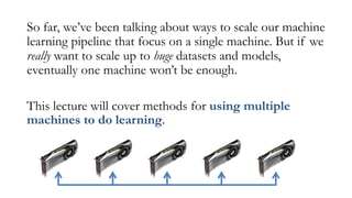
So far, we’vebeen talking about ways to scale our machine
learning pipeline that focus on a single machine. But if we
really want to scale up to huge datasets and models,
eventually one machine won’t be enough.
This lecture will cover methods for using multiple
machines to do learning.
3.
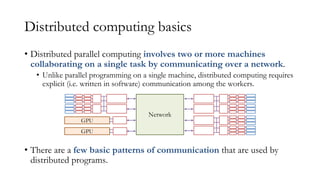
Distributed computing basics
•Distributed parallel computing involves two or more machines
collaborating on a single task by communicating over a network.
• Unlike parallel programming on a single machine, distributed computing requires
explicit (i.e. written in software) communication among the workers.
• There are a few basic patterns of communication that are used by
distributed programs.
Network
GPU
GPU
4.
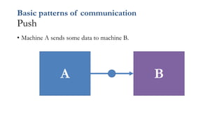
Basic patterns ofcommunication
Push
• Machine A sends some data to machine B.
A B
5.
Basic patterns ofcommunication
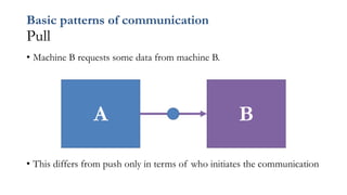
Pull
• Machine B requests some data from machine B.
• This differs from push only in terms of who initiates the communication
A B
6.
Basic patterns ofcommunication
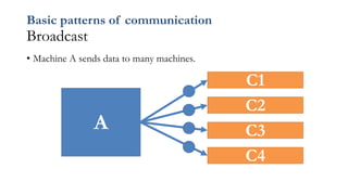
Broadcast
• Machine A sends data to many machines.
A
C1
C2
C3
C4
7.
Basic patterns ofcommunication
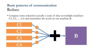
Reduce
• Compute some reduction (usually a sum) of data on multiple machines
C1, C2, …, Cn and materialize the result on one machine B.
C1
C2
C3
C4
B
8.
Basic patterns ofcommunication
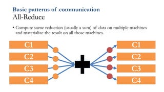
All-Reduce
• Compute some reduction (usually a sum) of data on multiple machines
and materialize the result on all those machines.
C1
C2
C3
C4
C1
C2
C3
C4
9.
Basic patterns ofcommunication
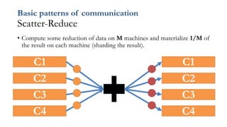
Scatter-Reduce
• Compute some reduction of data on M machines and materialize 1/M of
the result on each machine (sharding the result).
C1
C2
C3
C4
C1
C2
C3
C4
10.
Basic patterns ofcommunication
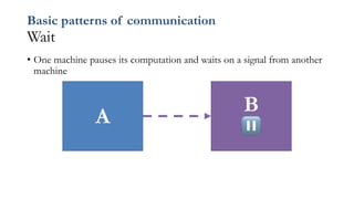
Wait
• One machine pauses its computation and waits on a signal from another
machine
A
B
⏸
11.
Basic patterns ofcommunication
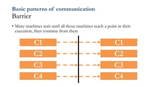
Barrier
• Many machines wait until all those machines reach a point in their
execution, then continue from there
C1
C2
C3
C4
C1
C2
C3
C4
12.
Patterns of CommunicationSummary
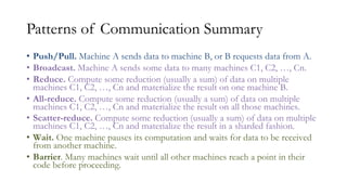
• Push/Pull. Machine A sends data to machine B, or B requests data from A.
• Broadcast. Machine A sends some data to many machines C1, C2, …, Cn.
• Reduce. Compute some reduction (usually a sum) of data on multiple
machines C1, C2, …, Cn and materialize the result on one machine B.
• All-reduce. Compute some reduction (usually a sum) of data on multiple
machines C1, C2, …, Cn and materialize the result on all those machines.
• Scatter-reduce. Compute some reduction (usually a sum) of data on multiple
machines C1, C2, …, Cn and materialize the result in a sharded fashion.
• Wait. One machine pauses its computation and waits for data to be received
from another machine.
• Barrier. Many machines wait until all other machines reach a point in their
code before proceeding.
13.
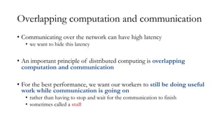
Overlapping computation andcommunication
• Communicating over the network can have high latency
• we want to hide this latency
• An important principle of distributed computing is overlapping
computation and communication
• For the best performance, we want our workers to still be doing useful
work while communication is going on
• rather than having to stop and wait for the communication to finish
• sometimes called a stall
14.
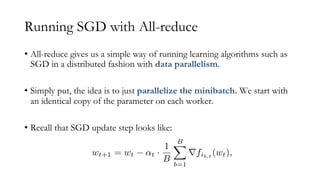
Running SGD withAll-reduce
• All-reduce gives us a simple way of running learning algorithms such as
SGD in a distributed fashion with data parallelism.
• Simply put, the idea is to just parallelize the minibatch. We start with
an identical copy of the parameter on each worker.
• Recall that SGD update step looks like:
1 2 n
ne machine pauses its computation and waits for data to be received from anot
ng over the network can have high latency, so an important principle of para
g computation and communication. For the best performance, we want
useful work while communication is going on (rather than having to stop an
n to finish).
GD with all-reduce. All-reduce gives us a simple way of running learning a
istributed fashion. Simply put, the idea is to just parallelize the minibatch. W
of the parameter wt on each worker. If the SGD update step is
wt+1 = wt ↵t ·
1
B
B
X
b=1
rfib,t
(wt),
15.
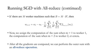
Running SGD withAll-reduce (continued)
• If
• Now, we assign the computation of the sum when m = 1 to worker 1,
the computation of the sum when m = 2 to worker 2, et cetera.
• After all the gradients are computed, we can perform the outer sum with
an all-reduce operation.
identical copy of the parameter wt on each worker. If the SGD update step is
wt+1 = wt ↵t ·
1
B
B
X
b=1
rfib,t
(wt),
and there are M worker machines such that B = M · B0
, then we can re-write this up
wt+1 = wt ↵t ·
1
M
M
X
m=1
1
B0
B0
X
b=1
rfim,b,t
(wt).
Now, we assign the computation of the sum when m = 1 to worker 1, the computa
m = 2 to worker 2, et cetera. After all the gradients are computed, we can perform
1
copy of the parameter wt on each worker. If the SGD update step is
wt+1 = wt ↵t ·
1
B
B
X
b=1
rfib,t
(wt),
e are M worker machines such that B = M · B0
, then we can re-write this update step as
wt+1 = wt ↵t ·
1
M
M
X
m=1
1
B0
B0
X
b=1
rfim,b,t
(wt).
e assign the computation of the sum when m = 1 to worker 1, the computation of the su
o worker 2, et cetera. After all the gradients are computed, we can perform the outer sum
1
16.
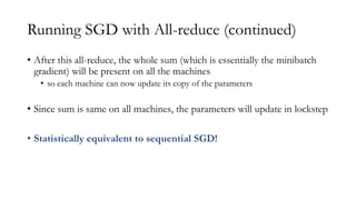
Running SGD withAll-reduce (continued)
• After this all-reduce, the whole sum (which is essentially the minibatch
gradient) will be present on all the machines
• so each machine can now update its copy of the parameters
• Since sum is same on all machines, the parameters will update in lockstep
• Statistically equivalent to sequential SGD!
17.
will be thesame. This corresponds to the following algorithm.
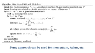
Algorithm 1 Distributed SGD with All-Reduce
input: loss function examples f1, f2, . . ., number of machines M, per-machine minibatch size B0
input: learning rate schedule ↵t, initial parameters w0, number of iterations T
for m = 1 to M run in parallel on machine m
load w0 from algorithm inputs
for t = 1 to T do
select a minibatch im,1,t, im,2,t, . . . , im,B0,t of size B0
compute gm,t
1
B0
B0
X
b=1
rfim,b,t
(wt 1)
all-reduce across all workers to compute Gt =
M
X
m=1
gm,t
update model wt wt 1
↵t
M
· Gt
end for
end parallel for
return wT (from any machine)
It is straightforward to see how one could use the same all-reduce pattern to run variants of SGD such as
Same approach can be used for momentum, Adam, etc.
18.
What are thebenefits of
distributing SGD with all-reduce?
What are the drawbacks?
19.
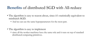
Benefits of distributedSGD with All-reduce
• The algorithm is easy to reason about, since it’s statistically equivalent to
minibatch SGD.
• And we can use the same hyperparameters for the most part.
• The algorithm is easy to implement
• since all the worker machines have the same role and it runs on top of standard
distributed computing primitives.
20.
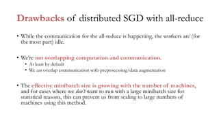
Drawbacks of distributedSGD with all-reduce
• While the communication for the all-reduce is happening, the workers are (for
the most part) idle.
• We’re not overlapping computation and communication.
• At least by default
• We can overlap communication with preprocessing/data augmentation
• The effective minibatch size is growing with the number of machines,
and for cases where we don’t want to run with a large minibatch size for
statistical reasons, this can prevent us from scaling to large numbers of
machines using this method.
21.
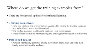
Where do weget the training examples from?
• There are two general options for distributed learning.
• Training data servers
• Have one or more non-worker servers dedicated to storing the training examples
(e.g. a distributed in-memory filesystem)
• The worker machines load training examples from those servers.
• These servers can handle preprocessing and data augmentation (but usually don’t)
• Partitioned dataset
• Partition the training examples among the workers themselves and store them
locally in memory on the workers.
The Basic Idea
•Recall from the early lectures in this course that a lot of our theory talked
about the convergence of optimization algorithms.
• This convergence was measured by some function over the parameters at time t
(e.g. the objective function or the norm of its gradient) that is decreasing with t,
which shows that the algorithm is making progress.
• For this to even make sense, though, we need to be able to talk about the
value of the parameters at time t as the algorithm runs.
• E.g. in SGD, we had
rver model. Recall from the early lectures in this course th
rgence of optimization algorithms. This convergence was meas
time t (e.g. the objective function or the norm of its gradient) t
e algorithm is making progress. For this to even make sense, t
value of the parameters at time t as the algorithm runs. E.g. in
wt+1 = wt ↵trfit
(wt)
24.
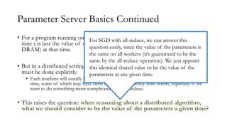
Parameter Server BasicsContinued
• For a program running on a single machine, the value of the parameters at
time t is just the value of some array in the memory hierarchy (backed by
DRAM) at that time.
• But in a distributed setting, there is no shared memory, and communication
must be done explicitly.
• Each machine will usually have one or more copies of the parameters live at any given
time, some of which may have been updates less recently than others, especially if we
want to do something more complicated than all-reduce.
• This raises the question: when reasoning about a distributed algorithm,
what we should consider to be the value of the parameters a given time?
For SGD with all-reduce, we can answer this
question easily, since the value of the parameters is
the same on all workers (it’s guaranteed to be the
same by the all-reduce operation). We just appoint
this identical shared value to be the value of the
parameters at any given time.
25.
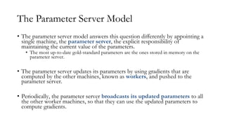
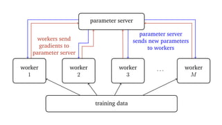
The Parameter ServerModel
• The parameter server model answers this question differently by appointing a
single machine, the parameter server, the explicit responsibility of
maintaining the current value of the parameters.
• The most up-to-date gold-standard parameters are the ones stored in memory on the
parameter server.
• The parameter server updates its parameters by using gradients that are
computed by the other machines, known as workers, and pushed to the
parameter server.
• Periodically, the parameter server broadcasts its updated parameters to all
the other worker machines, so that they can use the updated parameters to
compute gradients.
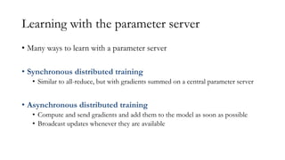
Learning with theparameter server
• Many ways to learn with a parameter server
• Synchronous distributed training
• Similar to all-reduce, but with gradients summed on a central parameter server
• Asynchronous distributed training
• Compute and send gradients and add them to the model as soon as possible
• Broadcast updates whenever they are available
28.
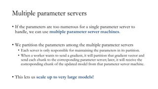
Multiple parameter servers
•If the parameters are too numerous for a single parameter server to
handle, we can use multiple parameter server machines.
• We partition the parameters among the multiple parameter servers
• Each server is only responsible for maintaining the parameters in its partition.
• When a worker wants to send a gradient, it will partition that gradient vector and
send each chunk to the corresponding parameter server; later, it will receive the
corresponding chunk of the updated model from that parameter server machine.
• This lets us scale up to very large models!
29.
Other Ways ToDistribute
The methods we discussed so far distributed across the minibatch (for all-reduce SGD)
and across iterations of SGD (for asynchronous parameter-server SGD).
But there are other ways to distribute that are used in practice too.
30.
Distribution for hyperparameteroptimization
• This is something we’ve already talked about.
• Many commonly used hyperparameter optimization algorithms, such as
grid search and random search, are very simple to distribute.
• They can easily be run on many parallel workers to get results faster.
31.
Model Parallelism
• Mainidea: partition the layers of a neural network among different worker
machines.
• This makes each worker responsible for a subset of the parameters.
• Forward and backward signals running through the neural network during
backpropagation now also run across the computer network between the
different parallel machines.
• Particularly useful if the parameters won’t fit in memory on a single machine.
• This is very important when we move to specialized machine learning accelerator
hardware, where we’re running on chips that typically have limited memory and
communication bandwidth.
32.
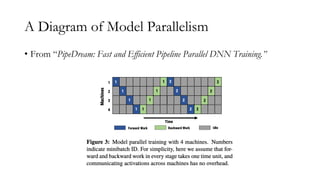
A Diagram ofModel Parallelism
• From “PipeDream: Fast and Efficient Pipeline Parallel DNN Training.”
33.
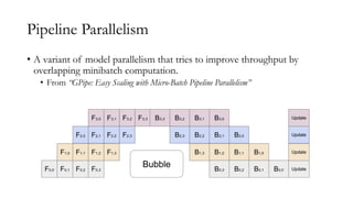
Pipeline Parallelism
• Avariant of model parallelism that tries to improve throughput by
overlapping minibatch computation.
• From “GPipe: Easy Scaling with Micro-Batch Pipeline Parallelism”
34.
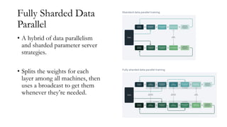
Fully Sharded Data
Parallel
•A hybrid of data parallelism
and sharded parameter server
strategies.
• Splits the weights for each
layer among all machines, then
uses a broadcast to get them
whenever they’re needed.
35.
Conclusion and Summary
•Distributed computing is a powerful tool for scaling machine
learning
• We talked about a few methods for distributed training:
• Minibatch SGD with All-reduce
• The parameter server approach
• Model parallelism
• And distribution can be beneficial for many other tasks too!