This document is a final report from 1993 on modelling and designing scalable parallel computing systems. It details the development of a fractal parallel computer topology that can extend to fill a wafer. Algorithms were developed for routing and load balancing, and a simulation program tested a 64-node network using UNIX and PC workstations. Benchmarking of a 16-node example network demonstrated scalability. The report discusses implementing hardware control to support applications using wafer-scale integration.


![2 INTRODUCTION 3
2 Introduction
2.1 Project Overview and Aim
This overview is as a brief outline of concepts of parallelism and its natural evolution in computer
science. The general aim is to justify wafer scale integration (WSI).
2.1.1 The Evolutionary Architecture of Computing Systems
With the advent of man’s searching for logical solutions and explanations to all his problems,
ideas were either dismissed as being correct or false. Yes-No logic became the order of the day
and the first binary computers utilised electro-mechanical relays to achieve simple functionality.
Operational parallelism existed even in the first generation of valve technology computers such
as ACE and DEUCE, which were made by NPL and English Electric. Closely followed by IBM’s
701 and 704 which used parallel arithmetic units. The 704 had six I/O channels added and was
renamed the IBM 709 and became an early best seller. Valve computing systems allowed ideas to
evolve, but it was not until systems were re-engineered to utilise the newly developed transistor
that any realistic demand outside research began to drive system development forward. The first
transistorised computer was born, when the existing IBM 709 thermionic valve computer was
re-engineered in transistor technology. The Ferranti ATLAS computer used logic and special
parallel features such as multiple ALU’s, registers, and memories, etc. The ATLAS Laboratory,
part of SERC’s Rutherford Appleton Laboratory offered a National service on one of these
machines. A more detailed general background can be gained from citation 2 of the bibliography.
Main-frame microcomputers led to centralised systems and the birth of super computers, which
forced circuit designers and material scientists to develop more integrated architectures. A spin-
off from this was the microprocessor, which acted as the heart of personal computers and led
to mass buying of small scale computing systems. Further integration spawned the single-chip
computer (e.g. the INMOS Transputer), and co-processing in workstations.
2.1.2 The birth of mainstream parallelism
Since then the quest for faster more efficient computing has led to the further exploitation of
hardware parallelism. The idea of processor arrays, farms and other such systems has grown
out of the use of networked computational facilities together with the ability to fabricate VLSI
processor chips, such as the INMOS Transputer (figure 1).
All these developments have included increasing degrees of parallelism in architecture, logic,
and programming. Research is tending to divide into two main areas, firstly computational
processing farms and arrays, and secondly the harnessing of existing facilities (figure 2) using
sophisticated software [1]. Diverse applications can then be run with the view towards parallel
computation for very large scale applications.
There is a search for common links between software parallelism and hardware parallelism, which
will lead to tightly coupled systems. Thus the consequential exploitation of circuit integration
on a wafer level, to reduce size, power consumption, and cost, whilst increasing reliability and
scalable computing power, is suggested as a consequence.](https://image.slidesharecdn.com/9523658a-d6cc-404b-a9db-06bb39c02657-150822223441-lva1-app6892/85/T401-7-320.jpg)
![2 INTRODUCTION 4
Figure 1: The INMOS T800 Transputer Architecture.
2.1.3 General Aim of the Project
The main project objective is therefore to establish the viability of a wafer scale integration
(WSI) approach to Parallel Computing Systems. The considerations for future system devel-
opment also encompass parallelising hardware functionality and to confirm present ideas on
parallel software harnessing [2] and the need for a single portable software platform [3]. The
author proposes a hierarchical machine built from physically distributed-memory WSI computer
elements, but is this feasible?
(figure 2)
It would seem that processing functions of addition, subtraction and multiplication have reached
their most advanced state, in that only two or three clock cycles are needed to carry out such
tasks. Hardware development now has to cope with data storage problems, such as global
addressability and access times. This will probably lead to further development of hierarchical
caching as in the Stanford DASH [4] project, so too the KSR [5],[6] machine with hardware
communication and global memory address space. Some sort of vector code addressing is not
to be ruled out. This has studied extensively by the author and the results will be presented at
a later date. Complete memory addressability and single event time are vital requirements of a
WSI multi-processor computer element. Similar timing problems occur in high speed processor
chips.
Memory locations in the DASH (figure 3) may be in one of the three states.
1. uncached - not cached by any cluster.
2. shared - in an unmodified state in the caches of one or more clusters.
3. dirty - modified in a single cache of some cluster.](https://image.slidesharecdn.com/9523658a-d6cc-404b-a9db-06bb39c02657-150822223441-lva1-app6892/85/T401-8-320.jpg)


![2 INTRODUCTION 7
Figure 5: Finite Element Analysis.
allocating the excess work to peripheral processors.
The effect of running processes in parallel seems to naturally lead to differential processor load-
ings, such as in the idle periods of a finite element analysis problem (where computational regions
of space are of different sizes). If it were not for dynamic load balancing [7], then the resultant
computational attainment would be much lower than is realisable.
The aim of the project is thus to consider the following areas, which require work when inte-
grating current parallel computing concepts into a wafer scale processing element.
1. Communication
The routing method used has to be addressed. Header stripping at a node is also an
important issue, along with the header structure for recognition purposes. These additional
ideas should be included in any WSI approach.
2. Network topology
Networks should be scalable and versatile. All-to-all routing can only be considered for
small farms of processors. Where possible the topology should in general allow flexible
reconfiguration.
3. Global and hierarchical address space
Indexing methods for global communication should be considered. Work has been done in
the context of the Stanford DASH [4] and KSR machine [5],[6] projects.
4. Global event times
In order to improve the integrity of data during its flow about a parallel computer system,
event timings are necessary. The INMOS T9000 [22] has an Event Bus built in for such
purposes.](https://image.slidesharecdn.com/9523658a-d6cc-404b-a9db-06bb39c02657-150822223441-lva1-app6892/85/T401-11-320.jpg)
![2 INTRODUCTION 8
5. I/O, control and inter-element communications
Extra handshaking signals to develop communication within a computer system may be
used.
6. Portable software interface
The make-up of parallel language extensions is in the process of being standardised. (See
Fortnet [2], F-Code [3], MPI[7], and HPF[8]).
2.2 Overall Objective
The overall objective of this project is to study the feasibility of using WSI in parallel computer
systems and necessary features to support software layering to allow for application portability
from existing systems to new ones.
A large scale application (LSA) consists of an assembly of program blocks usually with complex
inter-relationships. This can be represented on paper by a block flow diagram. The solution
to easier implementation of LSA’s is to be found through a three pronged attack, firstly the
development of Scalable Computing Systems (SCS’s), which can run diverse, but similar, ap-
plications, with increased efficiency. This is the job of the system architect. Secondly, the
computer programmers must be able to write their applications in such a way as to utilise the
full architectural potential, which brings us to the third and a very important aspect, namely the
compiler, which must allow the programmers to fulfil their goal. During the latter development
the compiler expert must make suggestions to the systems architect to incorporate adaptability
into the machine and software, in a way different to the stages of traditional compiler design.
Why adopt a three pronged attack? It is necessary because a complex functional system cannot
be made more efficient by a single isolated approach. Any application can be run on a specially
constructed machine, the specialisation approach towards an ideal solution. The demise of such
a system is the need for costly adaptation to solve a new problem. At the other end of the
imaginary scale is the totally versatile virtual machine, which would be so complex, that its
construction is, to all intents and purposes, a non-starter, which is why it was referred to as
being virtual.
2.2.1 Networks for Data Communication Channels
The answer lies with SCS’s, during the design of which the topics of processor array topol-
ogy and data routing are all studied to try and find some intermediate machine architectures.
Switched processor networks can be of varying topologies, such as: mesh; cube; hierarchical and
re-configurable (See figure 6). A network can be considered to be a topological assembly of in-
terconnected centres, which may comprise of high density nodal routing centres, down to simple
system termination sites. Features such as branches and loops may be seen in the networks
above.
Networks can be extremely diverse in overall topology, leading to different node co-ordination
numbers (the number of nearest neighbours to a node), as can be seen above.
Machine architecture constrains topological possibilities for mapping software, which dictate the
method(s) of routing, which will give optimum performance. For optimal program execution,
there is a corresponding topology for each program block. This given virtual topology will
generally define an optimal routing algorithm, and it must be mapped onto the physical processor
network. Thus if re-configurability of virtual topology and mapping is aimed for, then there is
a necessity for dynamic routing algorithms, which can take care of any topological changes. If](https://image.slidesharecdn.com/9523658a-d6cc-404b-a9db-06bb39c02657-150822223441-lva1-app6892/85/T401-12-320.jpg)

![2 INTRODUCTION 10
2.3.2 Load balancing
Load balancing within program blocks, which will determine the extent of the implementation
being parallel or serial, will also have an input to the topological mapping function of the
program on to the system architecture. Any load balancing of blocks must result in no change
to the program logic.
2.3.3 Least step evaluation
Route Cost Evaluation (RCE) should look at the least step cost evaluation of moving given data
via the quickest accessible route compared to the shortest known route. This can form the basis
for deciding the level of integrity of the route and whether it is an efficient channel for the data
transmission.
2.3.4 Three dimensional geometry
It has been clear for some time, that this area must be studied in order to find out about the
effects of levels of hierarchy and the number of nodal links.
2.3.5 System scalability
At least LOG(P) maximum routing distance must be achieved, without increasing the number
of links per node. In this case mathematical scalability of a large number of algorithms can be
achieved. Algorithms scaling as LOG(P) or better fall in class NC (or Nick’s Class, after Nick
Pippenger) of efficient methods [10]. Practical implementations of scalable computers can be
achieved in this way - Valient’s Thesis [11].
2.3.6 System reliability (Fault Tolerance)
To this end simulations will be carried out with the test software using dynamic topology. An
estimate of the communications efficiency of the network will be obtained and how this varies
as processors are killed off at random, to simulate system degeneration and failure.
2.3.7 Wafer Scale Integration
The possibility of implementation using current WSI technology is considered. Is it possible?
What restrictions does present technology impose?
2.3.8 Conclusions and future development
Data is collated and trends inferred to formulate conclusions and determine future directions to
be considered.](https://image.slidesharecdn.com/9523658a-d6cc-404b-a9db-06bb39c02657-150822223441-lva1-app6892/85/T401-14-320.jpg)
![3 NETWORKS IN GENERAL 11
3 Networks in General
Networks have come into existence through the need to communicate data between nodes.
The distance over which data is communicated, determines the network’s internal coupling. A
wide area network (WAN) is concerned with relatively isolated sites (e.g. a national digital
communications network) between which communication is relatively slow due to heavy-weight
protocol.
Each node may itself consist of a single processing element or a number of such elements con-
nected by a local area network (LAN). The latter is typically used by business or research
establishments to provide communications for internal site use only and provides fast commu-
nications over small distances.
The networks considered in this work are however even more tightly coupled and can be envisaged
to be within the same office or computer hall. Such networks would be used for wiring any printed
circuit board (PCB) used in connecting processors of a computer.
3.1 Networks and Hierarchical Properties
The degree of coupling in a network must be considered, as there is an upper limit on the
speed of electronic signals of 3x10⁸ ms-1. Thus in 1 nano-second (10-9 s) a signal can travel
30cm (approximately 1 foot). The time interval chosen is the equivalent to 1 clock pulse of a
1GHz clock (this is the upper limit). Normal clock frequencies are around 50 to 150 MHz or
equivalent distances of 6m down to 2m respectively. Hence for normal systems with connections
under these distances there is no problem. As the distance reduces with increasing clock speed,
problems begin to arise with large scale machines, where busses approach and get longer than
this limiting distance. Hence the clock cannot be globally correct.
If data is called over a large distance, much data can be in transit during periods where processing
has to be idle. Any influences on the transmission medium may bring about the corruption
of data and the subsequent need for re-transmission. Long transit times may be hidden by
processing cladding, if there is no need to use the data being transmitted during the processing
(i.e. it is sent ahead of time.)
The performance of a network is only good if it can cope with worst case loading and still achieve
the necessary throughput rates. This determines its usefulness for suitable channelling of data
between systems.
3.2 Arrays and Topology
(figure 7)
If any software can be topologically mapped onto a standard machine architecture, then a stan-
dard routing algorithm can be used, which contains optimisation parameters to help eliminate
hot-spots and keep the average step-path length to a minimum. It is however closely related
to the topology of the machine and as such is influenced by quantities such as maximum path
length and the number of links emanating from a node. A paper on MInimum DIstance MEsh
with Wrap-around links (MIDIMEW [12]) was one of the first sources in looking at ways of
reducing the maximum route length. It soon became clear that few system topologies reach the
LOG(P) hypercube limit, but it was also clear that a hypercube is not scalable for very large
systems, as the number of links into each node also increases, as LOG(P). It was at this stage
that the Erlangen 85 PMM Project [13] became of interest, since its architecture is quite similar](https://image.slidesharecdn.com/9523658a-d6cc-404b-a9db-06bb39c02657-150822223441-lva1-app6892/85/T401-15-320.jpg)

![3 NETWORKS IN GENERAL 13
in some ways to the first system concept designed as part of the current project [14].
The construction of a tightly-coupled computer system may dictate that only a limited number
of set topologies can be achieved under the machine’s architecture.
3.3 System Bandwidth
System bandwidth is undoubtedly improved by reducing the average routing distance. This is
due to the use of fewer links to carry the same information, thus leaving additional communica-
tions capacity.
3.4 Hierarchical Data Routing
Professor A.Hey (Southampton University [15] ) touched upon the concept of communication
hot-spots due to topological constraints, if too simplistic a routing algorithm is used.
Many routing techniques which work well are based on a North-south-east-west approach (
Midimew (figure 7) and Erlangen 85 PMM Project(figure 7) ), where four link directions are
considered. This will be referred to later as ’x-y’ routing. A hierarchical approach leads to the
natural development of top layers of hardware, which can deal with I/O control. In a system
similar to the Erlangen project there might be any number of I/O channels between 17 and 81
from the top two layers. Scalability dictates that data must be handed down to subordinate
processing levels and this idea was used to great effect in the Erlangen project.
It was seen that the initial network considered in the present project has an inferior step scal-
ability to the one envisaged and experimental architectural concept improvements have got to
be made. Modifications had to be made to the software model employed to allow for superior
protocol layer additions and the more involved routing algorithm necessary. As yet only the
most direct routing possibilities have been considered, but budgeting should be brought into the
algorithm to see if greater routing flexibility leads to the elimination of hot-spots and results in
higher efficiencies.
Some of the key points that any routing algorithm must address are as follows.
i) The ability to be deadlock free ii) The efficient utilisation of system bandwidth iii) Short
direct routes iv) Addressability of nodes
Routing must cover ideas such as Worm-Holes and Virtual connections and arrive at some esti-
mate for Routing Cost Evaluation (RCE), which will have an input into the routing algorithm.
3.5 Load Balancing
RCE will help load balancing of the communication layer. Other problems arise when the
application is spread in part or as a whole, over many processing nodes and computation loads
are different. Optimal performance can only be achieved by a relatively simple solution of
dynamic load balancing between all nodes involved during the execution of the application (see
for instance [7]).](https://image.slidesharecdn.com/9523658a-d6cc-404b-a9db-06bb39c02657-150822223441-lva1-app6892/85/T401-17-320.jpg)
![4 A PROPOSAL FOR FRACTAL AND SCALABLE NETWORKS 14
Figure 9: 4-link Transputer Networks.
3.6 Parallelism and the future
Nearly all applications exhibit partial program parallelism, which leads to bottlenecks in the
data flow (where one calculation relies upon the input from more than one previously calculated
result), thus not allowing optimal performance of the application to be reached. If a program
is looked at as being data flow through a complex pipe network, some generalisations can be
made. For optimal performance data handling by nodes must be equally balanced, to this end
the loading of each node must be calculated during the execution of the program, so that the
data loading on each node can be adjusted to re-establish load equilibrium over the nodes of the
system. This technique is referred to as dynamic load balancing [7].
The solution to these problems lies somewhere within the realms of mapping theory, but some
constraint will be applied by system architecture. To keep system bandwidth high, the paths
between nodes which communicate frequently, must be as small as possible.
4 A Proposal for Fractal and Scalable Networks
4.1 A Fractal Network; The Birth
Given that present transputers manufactured by INMOS have only four serial links, it was
decided that their possible interconnections should be studied. This would allow a working
machine to be built and tested using existing components. Modelling of the network could also
be done on existing transputer arrays (See figure 9).
After 4 processors were connected as above (See figure 9), this became a scalable fractal network,
because it resulted in a new unit with four free links as the original transputer had and therefore](https://image.slidesharecdn.com/9523658a-d6cc-404b-a9db-06bb39c02657-150822223441-lva1-app6892/85/T401-18-320.jpg)
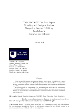
![4 A PROPOSAL FOR FRACTAL AND SCALABLE NETWORKS 16
Figure 11:
Such indexing is also a good thing to look at for route cost evaluation (RCE). The routing vector
is known and as long as the size of the displacement vector does not exceed the size of the routing
vector with a budget constraining factor of say ’1+ROUND[sqrt(Routing Vector)-log2(Routing
Vector)]’ added to the routing vector.
An example of an array with the TACTIC indexing given explicitly is now shown below.
See figure 12 above figure shows a TACTIC 0 16-node network with the decimal equivalents of
the binary addresses. The tetrahedra can be joined in a fractal fashion to extend the system
over a wafer of approximately 10cm diameter using 64 nodes. Why TACTICAL Indexing ? –
An example :
Choose two numbers between 0 and 63. e.g. 7 and 57
Let 7 be the source, which sends a message to 57 (the destination)
Now find the initial routing vector i.e. 57 - 7 = 50
Shortest route : travel along the diagonal:- Follow nodes on route 7 to 24 to 27 Sum of displace-
ment 0 17 20
Now travel as direct to 57, but perhaps we find 49 is blocked. Follow nodes on route 27 to 52
to 51 to 57 Sum of displacement 20 45 44 50
N.B. The final total displacement is the same as the routing vector even though the route was
not direct. This will always be true, no matter what route is taken, as long as the displacement
vector are always added for each link travelled along.
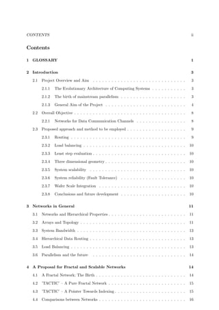
4.4 Comparisons between Networks
TACTIC 0 Torus Square Grid
Mean Path Length 2.19 2.13 2.66
Network Diameter 4 5 7](https://image.slidesharecdn.com/9523658a-d6cc-404b-a9db-06bb39c02657-150822223441-lva1-app6892/85/T401-20-320.jpg)


![5 NETWORK SIMULATION AND ALGORITHM 21
bridging link for the next level down and continues to test like this until an adjacent node
to the present position is found. This becomes the new source end and linking is carried
out until the highest level bridging link has been reached and crossed. The destination
side of the bridge becomes the new source and the whole procedure starts again.
2. Diagonal X/Y Routing Used with TACTIC 1 network
The Tactic 1 algorithm works out if there is a diagonal along which it can route. If there
is such a diagonal, then the nodes are tested in turn and unless a node is fully occupied,
the route will be set along the preferred diagonal. At the destination end of this diagonal
there is usually some ’x’ or ’y’ routing to carry out until the destination is reached.
N.B. If at any time a node is found to be fully occupied, then the simulation just chooses
two new numbers for the present route.
3. Vectorial Routing Used with TACTIC 1 network
This is the vectorial algorithm and it relies upon finding the largest vector (at a node) to
link towards the destination and can therefore start with ’x’ or ’y’ routing; followed by
diagonal routing, finishing with ’x’ or ’y’ routing.
4. Deadlock-Free Vectorial Routing Used with TACTIC 1 network
This is deadlock-free vectorial routing, as diagonal routing is not allowed after ’x’ or ’y’
routing. In order to guarantee deadlock freedom [16], each routing axis must be given a
priority, so that signal do not block each other.
General
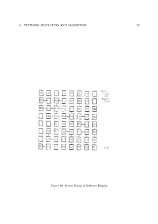
This is an example of screen printout from a personal computer (PC) showing a number of
typical routes between processors (See figure 16).
TX stands for a communicating node. S stands for a node acting as a switching point.
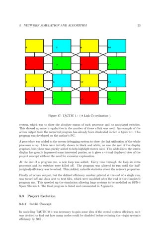
5.2 Towards Higher Network Bandwidth
Two configurations were analysed. Software modelling was first carried out with a new TAC-
TIC 1 configuration, which relies upon processors possessing eight link-directions plus a link-
umbilical. A second program was based around the skeleton of the first, but using the TACTIC
0 configuration, which had been the original concept of the project, but was superseded by TAC-
TIC 1 (See figure 17). TACTIC 0 (See figure 12) has less linking but a completely hierarchical
structure, which is fractal in nature.
The flow diagram shown previously, was drawn up for TACTIC 0, but used in aiding the program
structure of TACTIC 1 so that complete re-programming would not be necessary when changing
the configuration.
The routing strategy was set out and translated straight into C-coding, it was made to reduce
any diagonal differences first, then reduce in a linear manner until the destination was linked
up. In debugging the code the routing was checked against the expected paths based on the
processor vector address, and any program adjustments made.
On completion of a routing algorithm formalised in C-coding, a start was made on the modelling
of the complete parallel system. Attempts were made to debug the program by using printouts of
the routes used and number of processors talking, but the data so produced was too complex to
use. A program previously written by the author was used as the basis of the screen debugging](https://image.slidesharecdn.com/9523658a-d6cc-404b-a9db-06bb39c02657-150822223441-lva1-app6892/85/T401-25-320.jpg)


![7 INCREASED INTEGRATION 31
7.2 Exploration of Existing Technologies
1. INMOS transputer systems, and similar. All of these rely on off-wafer switching and do
not give much scope for large scale expansion.
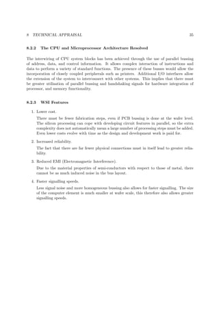
2. Links: It has been decided that it would be highly advantageous to remove the parallel-
serial link engines and use parallel linking. This will lead to increases in speed in excess
of a factor of 32.
3. Memory has been considered, whilst studying Open University course T393 and it will be
necessary to integrate some into the logical routing circuitry, in order that it might hold
the virtual routing look-up tables at nodes.
4. Wafer level switching, has been lumped together with the logical routing circuitry and has
been studied using software modelling.
5. T393 has suggested that multi-layer circuitry may be a limiting factor, but solutions are
possible for vertical tracks in a silicon wafer. The increased complexity of circuitry would
make additional processing viable, as processing power would also be increased.
6. Looking back at the last point: three dimensional bus layout design is going to be a highly
crucial step in the creation of wafer scale integrated devices (see following pages).
7. Catt Spiral and proposed Kernel Machine [17]: the current project extends these ideas
and considers them in the context of general purpose computing.
7.2.1 Bussing on a Wafer Scale
A few considerations of bus implementation are illustrated.
1. Shows an N-type bus in longitudinal cross-section.
2. Shows doping with N-type dopant to form a well.
3. Shows the over-doping with P-type dopant to fabricate a PN barrier.
4. Shows the final crossing point of the N-type busses, where the last N-type doping produces
the N-type bridging track.
Possible problems with doping and architecture
a) The number of over-doping stages will lead to problems of bus definition.
b) The actual crossing point produces a parasitic transistor pair.
Important :
These two effects are serious problems if such circuitry is to function correctly, without interfer-
ence.
7.2.2 Future Considerations
Heat dissipation from the wafer could be facilitated by using (5” long) aluminium cooling tubes,
creating a component looking rather like a hedgehog. Extra cooling can then easily be achieved
by using forced-air cooling over these tube arrays (Seee figure 26). Cooling of wafers is also an
area of future engineering research.](https://image.slidesharecdn.com/9523658a-d6cc-404b-a9db-06bb39c02657-150822223441-lva1-app6892/85/T401-35-320.jpg)

![8 TECHNICAL APPRAISAL 33
7.3 Reasons for WSI
The main aim of the project being undertaken, is to justify a hardware approach, via wafer scale
integration (WSI), to massively parallel machine architectures with complex topologies.
Most large-scale applications (LSA’s) include degrees of parallelism, for example: real-time pro-
cess control; image processing; complex scientific calculations, which at present are still run to
a large extent on various types of vector super-computers, which may or may not exhibit paral-
lelism at a very fundamental level. As a direct result of this sort of approach, achievable speed
is limited. Some programs which are not vectorisable to a high degree have only low efficiency.
This has led computer scientists to develop systems with explicit concurrency of processing
within the program structure and also massive parallelism in machine architectures. Simple
processor arrays (such as Intel i860 and INMOS Transputer systems) have already shown up
trends to increase the efficiency of selected applications, although still very limited in adaptation
and improvements.
A positive outcome to this project would lay down the skeleton for an easier approach to LSA’s
and far greater hardware support. This will be best served, if the resultant logic can be imple-
mented in ”Silicon”.
Study of system interconnection leads us to consider the field of network support. This is
mainly to deal with relatively long distance communications between centres of computation,
data storage, and system users. Network characteristics have constrained much of the possible
development, but as communications techniques improve and circuit integration increases, all
indications would seem to point towards the evolution of tightly coupled systems. Any evolution-
ary steps are being made from a gain in knowledge from experiences with workstation clusters
and transputer farms, which are both being managed by pseudo-parallel software harnesses.
It would seem to be financial forces which are steering system development, so that the next
logical transition is the virtual harnessing of workstation clusters for parallel processing purposes.
This is entirely due to the returns gained from volume sales and cost reductions emanating from
VLSI circuit fabrication techniques and volume production. Workstations themselves contain
several processors nowadays. There is the possibility of using WSI computer elements as the
basis for a workstation, which could then be clustered.
8 Technical Appraisal
8.1 Computing Systems
8.1.1 What do they do ?
Computing systems are used to manipulate data in a predefined manner as directed by a specific
application. The application will have requirements such as method, structure, semantics, and
syntax, which must be imparted to the computing system via machine code instruction sets,
which define system limitations. Such issues have been addressed, for instance, by F-Code [3], it
sets out clearly the ordering of data and operational functions to build up a strong, but flexible
software platform.](https://image.slidesharecdn.com/9523658a-d6cc-404b-a9db-06bb39c02657-150822223441-lva1-app6892/85/T401-37-320.jpg)
![8 TECHNICAL APPRAISAL 34
8.1.2 Software Developments
The development of a ’Portable Software Platform’ [2],[3],[4] has been done by various groups
to match applications to the available functionality required by a parallel system.
To allow for application portability between systems, without the need for time consuming
recoding, simple and efficient coding techniques are required.
The use of software message passing in the form of control signals, is made by harnesses (such as
Fortnet [2] and MPI[4]) which present to the global system signals for application management.
8.1.3 Hardware Developments
’Virtual Channel Routing’ (VCR) [18] considers all-to-all communication, which does not impose
too great a degree of constraint upon the system. VCR has been developed along the lines of
’Time-Space-Time’ switching of digital telephone networks.
As companies sell workstations to be used in clusters, they must develop the necessary parallel
software to support processing. Therefore the primary evolutionary steps will be dictated by
volume sales and not necessarily lead to an optimum solution.
8.1.4 General Developments
There are many areas which require large scale analysis and modelling, where much data com-
putation (and storage) is needed and would be ideally dealt with by a parallel computer. Such
parallel computers are gradually being developed, but in the meantime workstation clusters are
being used. These are controlled by software harnesses, which involve the use of message passing.
Massively parallel computing will find its major applications some time in the future. Currently
machines using between 64 and 1024 nodes suffice. Such machines are envisaged to take over
the place of workstation clusters, when all problems associated with parallel processing are
overcome.
8.2 Parallel Computing Systems and Scalability
8.2.1 A Problem in Data/Address/Event Communications
Until the problems of event timing and very large scale pooled memory addressability can be
resolved, using minimal latency overheads, massively parallel systems in the form of processor
arrays, or workstation clusters cannot feasibly be implemented in easily usable forms. An
example of simple software to run concurrent processes is Fortnet [2].
The degree to which a processor is isolated, is related to the distance from any extra communica-
tions channels as in a network. How to make the necessary information about event timings and
data addresses globally available to all processors involved with or interacting with a particular
application, becomes the priority question.](https://image.slidesharecdn.com/9523658a-d6cc-404b-a9db-06bb39c02657-150822223441-lva1-app6892/85/T401-38-320.jpg)
![9 DISCUSSION OF FUTURE NEEDS 36
9 Discussion of Future Needs
It has been difficult to limit the scope of this project ! However, as this project is not an end
in itself (or just another piece of routine academic work), every effort has been made to create
a fairly broad and stable platform for future research work envisaged by the author.
Any developments towards higher levels of program integration into parallel systems architec-
ture, must allow for easy methods of code translation, e.g. the development of editing tools like
”HeNCE”[19].
As much parallelism as possible should be contained in the machine code instructions. That is,
the use of parallelisation should be automatic, being invoked by code instructions. If a processor
becomes more heavily loaded than its nearest neighbours and is causing too much down time
elsewhere, then the system must be brought back into rough equilibrium.
The loading of each processor must be easily obtained from the global bus and cause the spawning
of the program step(s) required, with the subsequent transfer of work-load with the origin to
which reverse transfer of computed data may take place.
On the way towards a new universal program code (language) for parallel systems, it will be the
use of specialised compilers, which will determine the acceptability of systems development and
the portability of existing codes.
Communications across a parallel system require adequate bandwidth. The system should be
modular and thus network topology should have some basic building blocks.
Global address space and hierarchical caches should be looked at in the light of vectorial address-
ing, which along with the global event bus should allow greater control of concurrent functions.
Some new functions must be formed, which have automatic spawning capability. From a soft-
ware standpoint, a portable interface should be chosen for standardisation, which may then be
supported by hardware.
10 Conclusion and Further Development
WSI will place a need for more efficient communication of status for event timing and data
tagging. This could be done over extra global busses. At the time of writing, the INMOS T9000
(Transputer[22]) is becoming available for systems development, with its new event bus, which
acts as an umbilical connection to all transputers in the system.
Network topology has been modelled on a VCR machine using software routing, which has now
been integrated into a routing chip.
The TACTIC 0 configuration and hierarchical routing algorithm does constitute a fractal parallel
computing system, but bandwidth does not scale with system size. Layering this network with
control layers would seem to make significant differences to be looked at in future work.
8 link co-ordination gives greater bandwidth and also greater network efficiencies when routing.
A simple routing strategy as carried out by algorithm 1. This could be taken and made adaptive,
still trying to avoid deadlock, by using extra signalling busses if necessary.
It seems to be important to bring down the network diameter and increase the network band-
width, to lower message latencies by the shortening of routes.
A slow move towards WSI is certainly the way to increase the size of farms, arrays and clusters](https://image.slidesharecdn.com/9523658a-d6cc-404b-a9db-06bb39c02657-150822223441-lva1-app6892/85/T401-40-320.jpg)


![REFERENCES 39
References
12 Specific
[1] R.J.Allan ”Toward a Parallel Computing Environment for Fortran Applications on Par-
allel Computers” Theoretica Chimica Acta, special edition on Parallel Computing 84
(1993) 257-69
[2] ”Fortnet (3L) v1.0: Implementation and extensions of a message-passing harness for
transputers using 3L Parallel Fortran”, R.K.Cooper and R.J.Allan, Computer Physics
Communications 70(1992)521-543, North- Holland.
[3] a) ”F-Code: A Portable Software Platform for Data-Parallel Languages”,
A.B.Bolychevsky, V.B.Muchnick and A.V.Shafarenko, February 20, 1992.
b) ”The F-Code Abstract Machine and its Implementation”, Professor Chris Jesshope,
IEEE 1992 May 4-8.
[4] D.Lenoski, J.Laudon, K.Gharachorloo, W.-D. Weber, A.Gupta, J.Hennessy, M.Horowitz
and M.S.Lam ”The Stanford Dash Multiprocessor” IEEE Computer Magazine (March
1992) 63-79
[5] ”KSR Fortran Programming Manual” Kendall Square Research (February 1992)
[6] R.J.Allan, R.J.Blake and D.R.Emerson ”Early experiences of using the Kendall Square
KSR1 computer” Parallelogram (September 1992)
[7] ”The Development of a Two Dimensional Dynamic Load Balancing Strategy and Its
Implications”. University of West of England, M.Sc. Parallel Computing Systems, by
J.Garner, December 1992.
[8] Message Passin Interface Forum ”MPI Document for a Standard Message-Passing Inter-
face” (May 28,1993) document available by e-mail from netlib @orul.gov
[9] High Performance Fortran Forum ”High Performance Fortran Language Specification
v1.0” (3/5/93)
[10] N.Pippenger’s class of algorithms - see A.Gibbons and W.Rytter ”Efficient Parallel Al-
gorithms” (Cambridge University Press: 1989) ISBN 0-521-34585-5
[11] L.G.Valiant ”General Purpose Parallel Architectures” in J. van Leeuwen (ed.) ’Handbook
of Theoretical Computer Science’ (North Holland: 1990); ”A Bridging Model for Parallel
Computation” Communications of the ACM 33 (1990) 103-11
[12] ”An Optimal Topology for Multicomputer Systems based on a Mesh of Transputers”,
by A.Arruabarrena, R.Bevide, E.Herrada, J.L.Balcazar & C.Izu. published in Parallel
Computing (Pages 31 to 39, No 12, January 1990).
[13] ”A Tightly Coupled and Hierarchical Multiprocessor Architecture”, by W.Haendler,
A.Bode, G.Fritsch, W.Henning & J.Volkert. published in Computer Physics Commu-
nications (Pages 87 to 93, Vol 37, 1985).
[14] Page 13, T401 Project, Initial Report ”Modelling and Design of Scalable Computing
Systems Exhibiting Parallelism in Hardware and Software”
[15] Comments made during a seminar on ’Scalable Parallel Computing’ given by Professor
Anthony Hey, from Southampton University, on Monday January 12, 1993 at Daresbury
Laboratory.](https://image.slidesharecdn.com/9523658a-d6cc-404b-a9db-06bb39c02657-150822223441-lva1-app6892/85/T401-43-320.jpg)
![13 GENERAL 40
[16] ”Deadlock-Free Message Routing in Multiprocessor Interconnection Networks”, William
J.Dally and Charles L.Seitz. IEEE Transactions on Computers, Vol. C-36. No. 5. May
1987.
[17] a) I.Catt ”Wafer Scale Integration” Wireless World (July 1981) 37-8; ”Advance into the
Past” Wireless World (January 1984) p59;
b) ”Catt Spiral” Electronics and Wireless World (June 1988) p592;
c) ”The Kernel Logic Machine” Electronics and Wireless World (March 1989) 254-9
[18] a) ”The Virtual Channel Router”, M.Debbage, M.B.Hill, D.A.Nicole, University of
Southampton and A.Sturges (INMOS Ltd.), 1992 September 23.
b) ”Global Communications on locally-connected message-passing parallel computers”
M.Debbage, M.B.Hill and D.A.Nicole, 1992 October 13. accepted for publication in ’Con-
currency: Practice & Experience’.
[19] ”HeNCE, a user’s guide”, A.Begnelus, J.Dougarra, A.Geist, R.Manchek, K.Moore and
R.Wade. Oak Ridge National Laboratory. USA (November 1991).
13 General
[20] Past, Present, Parallel A Survey of Available Parallel Computing Systems, edited by
Arthur Trew & Greg Wilson, published by Springer-Verlag. 1991. ISBN 0-387-19664-1 /
ISBN 3-540-19664-1
[21] Parallel Computers 2, by Hockney & Jesshope, published by Adam Hilger. 1988. ISBN
0-85274-811-6(hbk) / ISBN 0-85274-812-4(pbk).
[22] IMS T9000 (Engineering Data), published for use by INMOS, 1993.
[23] IMS T800 transputer (Engineering Data), published for use by INMOS. January 1989.
[24] General Purpose MIMD Machines : High Performance Heterogeneous Interprocessor
Communication, ESPRIT Project 5404 (DS-Links). Technical Information, Published
by SGS-Thomson (INMOS). November 1992.
[25] HTRAM Specification, Revision 0, published by INMOS IQ Systems Division. June 16,
1992.
[26] SCI/Scalable Coherent Interface (Logical,Physical & Cache Coherence Specifications),
Draft Standard, published by IEEE. 1992.
[27] Data Formats/Shared Data Formats Optimized for Scalable Coherent Interface Proces-
sors, Draft Standard, published by IEEE. 1992.
[28] ”A Survey of Software Environments for Exploiting Networked Computing Resources”
Louis H.Turcotte, Engineering Research Center for Computational Field Simulation,
Mississippi State,MS 39762 USA (11/6/93).
14 Miscellaneous
INSPEC citations and abstracts searched through on the data-discs 1989-1992. list of searches
carried out on every disc :-](https://image.slidesharecdn.com/9523658a-d6cc-404b-a9db-06bb39c02657-150822223441-lva1-app6892/85/T401-44-320.jpg)

![15 APPENDIX 42
15 Appendix
15.1 C-CODE Source
15.1.1 GLOBAL LIBRARIES
#include ¡stdio.h¿ #include ¡time.h¿ #include ¡stdlib.h¿ #include ¡math.h¿
15.1.2 USER LIBRARY
#include ”define.h”
15.1.3 USER DEFINES
#define xxxx 10001 #define zzzz 1001 #define XXXX 100 #define ZZZZ 100 #define TTTT 1
15.1.4 RANDOM NUMBER GENERATOR
#include ”random.h”
15.1.5 GLOBAL ROUTINES
void T0(); void T1(); void T2(); void INFO(); void Ecubed(); void STATE();void REIN-
STAT();void INITIAL();void LOG(); void GOAL();void BEGIN();void Tvector(); void Dvec-
tor();void Lvector();void sort();void vec();void VALID(); void TWOZ();void POS();void DECO();void
NEWDIR();void STRATEGY(); void TACTICON();void ANTACTIC();void LINKER();void
INSTEP0(); void INSTEP1();void INSETUP(); void AVERAGE(); void AVE100();
15.1.6 GLOBAL VARIABLES
static int b, c, h, h1, l1, m1, q, s, w, tv, x, y, z; static int new, ref, scip, sign, take, vek,
procs, used, loop; static int count, size, xpos, ypos, colour, lastlinkdir, lastlinkrid; static int
deltaz, destination, move, delta, tim, present, logged, try; static int node, join, last, lone, rang,
toto, launch, lastlink, linklast; static int SET, DIR, RID, DIRT, FREE, TACTIC, Node, arr,
ARR; static int now, reached, tried, TIM, direction, exyte; static int joint[3], point[3], ivec[3],
jvec[3], ilev[3], jlev[3], vref[2]; static int inlet[3], outlet[3], posx[4], posy[4], level[3][4], con[2],
ncount[2]; static int vector[LINKS], dnode[2*LEVEL]; static int slot[PROCS][PROCS][NLINK],
source[PROCS]; static int occupied[PROCS][NLINK][2], parity[PROCS][NLINK][2]; static int
idest[LEVEL], ih[LEVEL], dif[LEVEL], vektor[LEVEL+1]; float ERLANGS, Erlangs, ave, rage,
AVE, RAGE; long erlangs, talk, link[PROCS]; float stats1, stats, dur, DUR;
15.1.7 MAIN PROGRAM
void main()](https://image.slidesharecdn.com/9523658a-d6cc-404b-a9db-06bb39c02657-150822223441-lva1-app6892/85/T401-46-320.jpg)
![15 APPENDIX 43
15.1.8 LOCAL VARIABLES & ROUTINES
static int n, txs; TEST();
exyte=0; /* Inputting of Program-DATA Variables */ TACTIC=TTTT; do { printf(”
n”); printf(”NOW RUNNING TACTIC [”);printf(”%1i”,TACTIC);printf(”] ROUTING STRAT-
EGY”); printf(”
n”);
/* Inputting of Program-DATA Variables */ for(l1=XXXX;l1¡xxxx;l1=l1*10){ printf(”
n”); printf(”Input Application Run Time : ”);printf(”%5i
n”,l1); for(b=ZZZZ;b¡zzzz;b=b*10){ printf(”
n”); printf(”Input MAXIMUM Message Time : ”);printf(”%5i
n”,b); for (w=0; w¡PROCS; ++w) {source[w]= -1;link[w]=0; for (x=0; x¡4; ++x) {for (y=0;
y¡2; ++y) {occupied[w][x][y]= -1;}}} printf(”
n”); BEGIN();
Erlangs=0;ave=0;rage=0;reached=0;tried=0;dur=0.00;TIM=0;stats1=0.00;
/* DATA-Collation Loop */ txs= -1;procs=PROCS; if(TACTIC==2 —— TACTIC==3)DECO();
do{txs=txs+1;if (txs¿=1){{ERLANGS=0; Erlangs=0;ave=0;rage=0;reached=0;tried=0;dur=0.00;TIM=0;}
15.1.9 END OF PROGRAM SET-UP
15.1.10 BEGINNING OF MAIN
/* Failling of Nodes during Test */ for (x=0; x¡1; ++x){ h=(PROCS-1)*uni();FREE=1;STATE(h,9);
if (FREE==1){ for(y=0; y¡4;++y){occupied[h][y][1]=9;occupied[h][y][0]=9;}} else x=x-1;}}
/* Statistical Averaging Loop */
for (loop=1; loop¡=100; ++loop){erlangs=0; for (s=0;s¡l1;++s){
/* Re-instating OFF-Line Processors */ if (s¿=1) REINSTAT(s); SET=0;
/* Processor-LINK Loop */ for(q=0;q¡100;++q){
/* Variable Initialisation */ if(q==0)INITIAL(); if(SET!=3){ if(q==0){++try;dur=dur+DUR;++TIM;}
if(TACTIC==0)T0(); if(TACTIC==1)T1(); if(TACTIC==2 —— TACTIC==3)T2(); }}}
/* NB. If NO Valid Vector Found Above, Regression to Previous Node {NOT YET} */
/* END of TRACKING LOOP */ for (s=l1; s¡l1+b+1; ++s)REINSTAT(s);} tried=tried+try;reached=1;ave=a
if(stats==0.00)stats=50*(rage/procs)/ave; stats1=100*(rage/procs)/ave;AVE=0;RAGE=0;ERLANGS=0;try=
used=0; /* Finds the Number of Communicating Nodes */ for(z=0; z¡procs; ++z){ FREE=1;STATE(z,9);if(FR
AVE100();}while(exyte==0 && used¡=39 && stats1¿=stats —— txs== -1); stats=0.00;stats1=0.00;txs=
-1;}}TACTIC=1+TACTIC;exyte=0; } while (TACTIC==0 —— TACTIC==1 —— TACTIC==2
—— TACTIC==3);}](https://image.slidesharecdn.com/9523658a-d6cc-404b-a9db-06bb39c02657-150822223441-lva1-app6892/85/T401-47-320.jpg)
![15 APPENDIX 44
15.1.11 END OF MAIN PROGRAM
15.1.12 SUB ROUTINES
/* Initialisation of Program Variables for Each Run */ void INITIAL() {static int z;{ for(z=0;z¡3;++z){point[z]=
inlet[z]=0;outlet[z]=0; for(x=0;x¡4;++x)level[z][x]=0;} new=0;vref[0]=0;vref[1]=0; for(z=0;z¡LEVEL;++z){dif
-1;} for (z = 0; z ¡2; ++z) { r1 = uni()*PROCS;joint[z]=r1;point[z]=r1;} DUR=b*uni();
if(b==0){DUR=0;tim=s+1;} else tim=DUR+1+s; last=0;lone=0;launch= -1; lastlinkdir=0;lastlinkrid=0;
destination=point[0];h=point[1];h1=point[1];SET=0; FREE=1;STATE(h1,8);STATE(h1,9); if
(destination!=h1 && FREE==1 && link[h1]¡=3) { LOG(h1,8,0);ARR=3;} else {SET=3;q=100;}}}
/* Re-instating OFF-Line Processors */ void REINSTAT(now) {static int a, c, x, y, z;{for (y=0;
y ¡PROCS; ++y) {a= -1;for (x=0; x ¡PROCS; ++x) { for (z=0; z ¡4; ++z) {if (slot[x][y][z]==now)
{ a=source[y];slot[x][y][z]=0; for (c=0; c¡2; ++c) {if (parity[x][z][c]==now) { DIR=occupied[x][z][c];
occupied[x][z][c]= -1;parity[x][z][c]=0; if (c==0) {link[x]=link[x]-1;}}}}}} if (a!= -1) {source[y]=
-1;}}}}
15.1.13 CONFIGURATION
void T0() /* Choose TACTIC 0 */ {h=joint[1];point[1]=h;point[2]=0;posx[2]=0;posy[2]=0; /*
TRACKING LOOP */ do { /* Routing Stratergy Taken */ STRATEGY(); /* LOG TAC-
TIC 0 Link Information */ VALID(h); if(SET==1)INFO(); if(present==2)SET=1; } while
(SET==0);}
15.1.14 CONFIGURATION
void T1() /* Choose TACTIC 1 */ {h=joint[1];point[1]=h;point[2]=0;posx[2]=0;posy[2]=0;
/* Find X & Y Values for SOURCE & DESTINATION */ for (z=0;z¡2;++z) {posx[z]=point[z]/8;posy[z]=point[
(8*posx[z]);}
/* Find DELTA : X & Y Values */ posx[2]=posx[0]-posx[1];posy[2]=posy[0]-posy[1];
/* SET Delta-Step X & Y Values */ INSTEP1();
/* Find NEW Values of X & Y for NEXT Switch in Link */ posx[3]=posx[1]+con[0];posy[3]=posy[1]+con[1];
/* Find Direction SET */ INSETUP();
/* Initialise Rotational Vector Algorithm (RVA) */ if (SET==0) {delta=0;sign=1;deltaz=sign*delta;DIRT=DIR
/* TRACKING LOOP */ present=0;x=0; do {present=0;z=0;x=x+1; do {z=z+1;
/* Find NEW Node if Valid : X & Y found */ new=(8*posx[3]+posy[3]); VALID(new); if(SET==1)h=new;
/* LOG Link Information */ if(SET==1)INFO(); else {z=100;x=100;} } while (delta¡=7 &&
present==0 && z¡=100); if(delta¿=8 && present==0){REINSTAT(tim);q=100;SET=3;} }
while (SET==0 && x¡=100);}
/* Choose TACTIC 10 */ void T2() { /* Find ALL Direction Vectors Around Present Node */
Dvector(h);
/* Taking ’Dvectors’ in Descending Order for the Translation */ /* Find Valid Link Vector to
Reduce the ’Tvector’ the Most */ Lvector();}](https://image.slidesharecdn.com/9523658a-d6cc-404b-a9db-06bb39c02657-150822223441-lva1-app6892/85/T401-48-320.jpg)
![15 APPENDIX 45
15.1.15 PROGRAM CALCULATIVE ROUTINES
void STRATEGY() FRACTAL ROUTING STRATEGY {static int u;{ /* Find X & Y Tactical-
Values (ALL 3 Levels) for SOURCE & DESTINATION */ /* NB. TACTICON finds the TAC-
TICAL Level Numbers */ do{ for (u = 0; u ¡2; ++u) {h=joint[u];TACTICON(u,h);} /* Find
DELTA : X & Y Tactical-Values */ for (u = 0; u ¡3; ++u) {level[u][2]=level[u][0]-level[u][1];} /*
SET Delta-Step X & Y Tactical-Values */ INSTEP0(); LINKER(); DIR=lastlinkdir;RID=lastlinkrid;
} while (move==0); h=joint[1];move=0;}}
/* LOG Link Information */ void INFO() { FREE=1;STATE(h,9);if(h==destination)STATE(h,8);
if(FREE==1 && SET==1){RID=DIR-4; if(RID¡= -1)RID=RID+8;FREE=1;STATE(m1,DIR);
if(FREE==1){LOG(m1,DIR,1);} else SET=2; STATE(h,RID);if(h==destination)STATE(h,8);
if(FREE==1){ LOG(h,RID,0); if(h==destination){ LOG(h,8,1);present=2; q=100;GOAL();}}
else SET=2;} else SET=2; if(SET==2){REINSTAT(tim);present=3;q=100;} logged=0; if(present==1)logged=
/* Find Status of a Node */ void STATE(node,direction) {static int t, u;{for (u=0; u¡4; ++u)
{for (t=0; t¡2; ++t) { if (occupied[node][u][t]==direction)FREE=0;}}}}
/* Logs ALL Relevant Data for a Node */ void LOG(node,direction,c) {static int z;{for (z=0; z¡4;
++z) { if (parity[node][z][c]==0) {slot[node][destination][z]=tim;if(c==0)++link[node]; source[destination]=h1
void INSTEP1() FOR FINDING POSITION CHANGES IN VECTOR {if (posx[2]¡=0) con[0]=-
1;else con[0]=1; if (posy[2]¡=0) con[1]=-1;else con[1]=1; if (posx[2]==0) con[0]=0; if (posy[2]==0)
con[1]=0;}
void INSETUP() FOR FINDING VECTOR DIRECTION FROM POSITION CHANGES {if
(con[0]== -1) { if (con[1]== -1)DIR = 3; if (con[1]== 0) DIR = 2; if (con[1]== 1) DIR=1;}
if (con[0]== 0) { if (con[1]== -1)DIR = 4; if (con[1]== 1) DIR = 0;} if (con[0]== 1) { if
(con[1]== -1)DIR = 5; if (con[1]== 0) DIR = 6; if (con[1]== 1) DIR = 7;} if (SET!=3)
{point[1]=joint[1];joint[1]=(8*posx[3])+posy[3];h=joint[1];m1=point[1];}}
/* Check for Violation of Array Boundary */ void VALID(node) {SET=1;if(node¡= -1 ——
node¿=procs)SET=2;}
void TACTICON(v,h) LOOK-UP TABLE {if (h==0)node=0;if (h==1)node=1;if (h==2)node=4;if
(h==3)node=5; if (h==4)node=16;if (h==5)node=17;if (h==6)node=20;if (h==7)node=21; if
(h==8)node=2;if (h==9)node=3;if (h==10)node=6;if (h==11)node=7; if (h==12)node=18;if
(h==13)node=19;if (h==14)node=22;if (h==15)node=23; if (h==16)node=8;if (h==17)node=9;if
(h==18)node=12;if (h==19)node=13; if (h==20)node=24;if (h==21)node=25;if (h==22)node=28;if
(h==23)node=29; if (h==24)node=10;if (h==25)node=11;if (h==26)node=14;if (h==27)node=15;
if (h==28)node=26;if (h==29)node=27;if (h==30)node=30;if (h==31)node=31; if (h==32)node=32;if
(h==33)node=33;if (h==34)node=36;if (h==35)node=37; if (h==36)node=48;if (h==37)node=49;if
(h==38)node=52;if (h==39)node=53; if (h==40)node=34;if (h==41)node=35;if (h==42)node=38;if
(h==43)node=39; if (h==44)node=50;if (h==45)node=51;if (h==46)node=54;if (h==47)node=55;
if (h==48)node=40;if (h==49)node=41;if (h==50)node=44;if (h==51)node=45; if (h==52)node=56;if
(h==53)node=57;if (h==54)node=60;if (h==55)node=61; if (h==56)node=42;if (h==57)node=43;if
(h==58)node=46;if (h==59)node=47; if (h==60)node=58;if (h==61)node=59;if (h==62)node=62;if
(h==63)node=63; level[2][v]=node/16;level[1][v]=(node-(16*level[2][v]))/4; level[0][v]=(node-(16*level[2][v])-
(4*level[1][v]));}
/* To FIND the TACTICAL-LINK Level & TACTICAL Output-Link */ void INSTEP0() {static
int u;{ for (u=0; u¡3; ++u) {if (level[2-u][2]==0)u=u; else {join=2-u;u=4;}} if (join==2){
LEVEL 2 if (level[2][2]== -3){ if (level[2][1]==3){outlet[2]=48;inlet[2]=15;}DIR=3;RID=7;} if
(level[2][2]== -2){ if (level[2][1]==2){outlet[2]=32;inlet[2]=10;} if (level[2][1]==3){outlet[2]=53;inlet[2]=31;}DI
if (level[2][2]== -1){ if (level[2][1]==1){outlet[2]=16;inlet[2]=5;DIR=4;RID=0;} if (level[2][1]==2){outlet[2]=3](https://image.slidesharecdn.com/9523658a-d6cc-404b-a9db-06bb39c02657-150822223441-lva1-app6892/85/T401-49-320.jpg)
![15 APPENDIX 46
if (level[2][1]==3){outlet[2]=58;inlet[2]=47;DIR=4;RID=0;}} if (level[2][2]== 1){ if (level[2][1]==0){outlet[2]=
if (level[2][1]==1){outlet[2]=26;inlet[2]=37;DIR=5;RID=1;} if (level[2][1]==2){outlet[2]=47;inlet[2]=58;DIR=
if (level[2][2]== 2){ if (level[2][1]==0){outlet[2]=10;inlet[2]=32;} if (level[2][1]==1){outlet[2]=31;inlet[2]=53;}D
if (level[2][2]== 3){ if (level[2][1]==0){outlet[2]=15;inlet[2]=48;}DIR=7;RID=3;}} if (join==1){
LEVEL 1 if (level[1][2]== -3){ if (level[1][1]==3){outlet[1]=12+16*level[2][0]; inlet[1]=3+16*level[2][0];}DIR=3
if (level[1][2]== -2){ if (level[1][1]==2){outlet[1]=8+16*level[2][0]; inlet[1]=2+16*level[2][0];} if
(level[1][1]==3){outlet[1]=13+16*level[2][0]; inlet[1]=7+16*level[2][0];}DIR=2;RID=6;} if (level[1][2]==
-1){ if (level[1][1]==1){outlet[1]=4+16*level[2][0]; inlet[1]=1+16*level[2][0];DIR=4;RID=0;} if
(level[1][1]==2){outlet[1]=9+16*level[2][0]; inlet[1]=6+16*level[2][0];DIR=1;RID=5;} if (level[1][1]==3){outlet
inlet[1]=11+16*level[2][0];DIR=4;RID=0;}} if (level[1][2]== 1){ if (level[1][1]==0){outlet[1]=1+16*level[2][0];
inlet[1]=4+16*level[2][0];DIR=0;RID=4;} if (level[1][1]==1){outlet[1]=6+16*level[2][0]; inlet[1]=9+16*level[2][
if (level[1][1]==2){outlet[1]=11+16*level[2][0]; inlet[1]=14+16*level[2][0];DIR=0;RID=4;}} if (level[1][2]==
2){ if (level[1][1]==0){outlet[1]=2+16*level[2][0]; inlet[1]=8+16*level[2][0];} if (level[1][1]==1){outlet[1]=7+16
inlet[1]=13+16*level[2][0];}DIR=6;RID=2;} if (level[1][2]== 3){ if (level[1][1]==0){outlet[1]=3+16*level[2][0];
inlet[1]=12+16*level[2][0];}DIR=7;RID=3;}} if (join==0){ LEVEL 0 if (level[0][2]== -3){ if
(level[0][1]==3){outlet[0]=3+16*level[2][0]+4*level[1][0]; inlet[0]=0+16*level[2][0]+4*level[1][0];}DIR=3;RID=
if (level[0][2]== -2){ if (level[0][1]==2){outlet[0]=2+16*level[2][0]+4*level[1][0]; inlet[0]=0+16*level[2][0]+4*lev
if (level[0][1]==3){outlet[0]=3+16*level[2][0]+4*level[1][0]; inlet[0]=1+16*level[2][0]+4*level[1][0];}DIR=2;RID
if (level[0][2]== -1){ if (level[0][1]==1){outlet[0]=1+16*level[2][0]+4*level[1][0]; inlet[0]=0+16*level[2][0]+4*lev
if (level[0][1]==2){outlet[0]=2+16*level[2][0]+4*level[1][0]; inlet[0]=1+16*level[2][0]+4*level[1][0];DIR=1;RID=
if (level[0][1]==3){outlet[0]=3+16*level[2][0]+4*level[1][0]; inlet[0]=2+16*level[2][0]+4*level[1][0];DIR=4;RID=
if (level[0][2]== 1){ if (level[0][1]==0){outlet[0]=0+16*level[2][0]+4*level[1][0]; inlet[0]=1+16*level[2][0]+4*lev
if (level[0][1]==1){outlet[0]=1+16*level[2][0]+4*level[1][0]; inlet[0]=2+16*level[2][0]+4*level[1][0];DIR=5;RID=
if (level[0][1]==2){outlet[0]=2+16*level[2][0]+4*level[1][0]; inlet[0]=3+16*level[2][0]+4*level[1][0];DIR=0;RID=
if (level[0][2]== 2){ if (level[0][1]==0){outlet[0]=0+16*level[2][0]+4*level[1][0]; inlet[0]=2+16*level[2][0]+4*lev
if (level[0][1]==1){outlet[0]=1+16*level[2][0]+4*level[1][0]; inlet[0]=3+16*level[2][0]+4*level[1][0];}DIR=6;RID
if (level[0][2]== 3){ if (level[0][1]==0){outlet[0]=0+16*level[2][0]+4*level[1][0]; inlet[0]=3+16*level[2][0]+4*lev
void LINKER() TACTICAL LEVEL LINKER {static int u;{node=inlet[join];ANTACTIC();lastlink=h;if(last==
node=outlet[join];ANTACTIC();linklast=h;if(lone==0){lone=h;rang=last;toto=lone;} if(joint[1]==lone
&& launch== -1){joint[0]=last; /* NB. TACTICON finds the TACTICAL Level Numbers */
for (u = 0; u ¡2; ++u) {h=joint[u];TACTICON(u,h);} /* Find DELTA : X & Y Tactical-Values
*/ for (u = 0; u ¡3; ++u) {level[u][2]=level[u][0]-level[u][1];} /* SET Delta-Step X & Y Tactical-
Values */ INSTEP0();m1=lone;joint[1]=last;joint[0]=point[0]; lastlinkdir=DIR;lastlinkrid=RID;
launch=last;lone=0;last=0;move=1;} else {if(joint[1]==linklast && move==0 && (launch== -
1 —— launch== -2)){ move=1;m1=joint[1];joint[1]=lastlink; if(join¡=1){node=inlet[join+1];ANTACTIC();link
lastlinkdir=DIR;lastlinkrid=RID;} else {if(launch!= -1) {move=1;m1=launch;launch= -2; if(joint[1]==toto)join
else { if(joint[1]==rang)joint[1]=lastlink; else joint[1]=linklast;} lastlinkdir=DIR;lastlinkrid=RID;}}
if(launch!= -2)joint[0]=linklast; else joint[0]=point[0];}}}
void ANTACTIC() LOOK-UP TABLE {if (node==0)h=0;if (node==1)h=1;if (node==4)h=2;if
(node==5)h=3; if (node==16)h=4;if (node==17)h=5;if (node==20)h=6;if (node==21)h=7; if
(node==2)h=8;if (node==3)h=9;if (node==6)h=10;if (node==7)h=11; if (node==18)h=12;if
(node==19)h=13;if (node==22)h=14;if (node==23)h=15; if (node==8)h=16;if (node==9)h=17;if
(node==12)h=18;if (node==13)h=19; if (node==24)h=20;if (node==25)h=21;if (node==28)h=22;if
(node==29)h=23; if (node==10)h=24;if (node==11)h=25;if (node==14)h=26;if (node==15)h=27;
if (node==26)h=28;if (node==27)h=29;if (node==30)h=30;if (node==31)h=31; if (node==32)h=32;if
(node==33)h=33;if (node==36)h=34;if (node==37)h=35; if (node==48)h=36;if (node==49)h=37;if
(node==52)h=38;if (node==53)h=39; if (node==34)h=40;if (node==35)h=41;if (node==38)h=42;if
(node==39)h=43; if (node==50)h=44;if (node==51)h=45;if (node==54)h=46;if (node==55)h=47;
if (node==40)h=48;if (node==41)h=49;if (node==44)h=50;if (node==45)h=51; if (node==56)h=52;if
(node==57)h=53;if (node==60)h=54;if (node==61)h=55; if (node==42)h=56;if (node==43)h=57;if
(node==46)h=58;if (node==47)h=59; if (node==58)h=60;if (node==59)h=61;if (node==62)h=62;if](https://image.slidesharecdn.com/9523658a-d6cc-404b-a9db-06bb39c02657-150822223441-lva1-app6892/85/T401-50-320.jpg)
![15 APPENDIX 47
(node==63)h=63;}
/* Find ALL Direction Vectors Around Present Node */ void Dvector(node) {static int x, y;{
TWOZ(node); for(x=0;x¡2;++x){ count=0; for(y=LEVEL;y¿=0;–y){ if(dnode[2*y+x]==dnode[x])++count;
else {if(count¿=1)count=0;}} if(count==LEVEL+1)count=LEVEL;ncount[x]=count+1;} if(dnode[0]==1){vec
= -1;vec(0);vector[0] = 1*size;} if(dnode[0]==0){vector[0] = 1;vec(0);vector[4] = -1*size;} if(dnode[1]==1){vect
= -2;vec(1);vector[6] = 2*size;} if(dnode[1]==0){vector[6] = 2;vec(1);vector[2] = -2*size;} vec-
tor[1]=vector[0]+vector[2];vector[3]=vector[2]+vector[4]; vector[5]=vector[4]+vector[6];vector[7]=vector[6]+vec
/* Convert Node Number to Binary */ void TWOZ(node) {static int cnode, enode, z; if(node¡=PROCS-
1){ cnode=node; for(z=0;z¡=(2*LEVEL-1);++z){ enode=cnode/2;dnode[z]=cnode-2*enode;cnode=enode;}}}
/* Finds Direction Vectors */ void vec(x) {static int w,y; size=0;y=2;for(w=0;w¡(ncount[x]-
1);++w){size=size+y;y=4*y;}size=size+1;}
/* Taking ’Dvectors’ in Descending Order for the Translation */ /* Find Valid Link Vector
to Reduce the ’Tvector’ the Most */ void Lvector() {present=0; do {sort();INFO();} while
(present==0);}
/* E-Cubed Routing (Deadlock Prevention) */ void Ecubed(DIR) {ARR=arr;if(TACTIC==3){
if(DIR==1 —— DIR==3 —— DIR==5 —— DIR==7)arr=2; if(DIR==2 —— DIR==6)arr=1;
if(DIR==0 —— DIR==4)arr=0;}}
/* Sorts Out Dvectors which will Reduce the Tvector */ void sort() {delta=LEVEL;Tvector();move=0;scip=0;
for(z=0;z¡=7;++z){ if(tv==vector[z]){Ecubed(DIR);if(ARR¿=arr){DIR=z;scip=1;z=8;}}} if(scip==0){
idest[LEVEL-1]=destination;ih[LEVEL-1]=h; for(delta=LEVEL-1;delta¿=1;–delta){ idest[delta-
1]=idest[delta]/4;ih[delta-1]=ih[delta]/4; dif[delta-1]=idest[delta-1]-ih[delta-1]; if(dif[delta-1]==0){
take=4*ih[delta-1]; idest[delta]=idest[delta]-take; ih[delta]=ih[delta]-take; vek=idest[delta]; ref=ih[delta];
delta=0;} else {vek=idest[0];ref=ih[0];}} if(ref==0){ if(vek==1)ivec[2]=0; if(vek==2)ivec[2]=6;
if(vek==3)ivec[2]=7;} if(ref==1){ if(vek==0)ivec[2]=4; if(vek==2)ivec[2]=5; if(vek==3)ivec[2]=6;}
if(ref==2){ if(vek==0)ivec[2]=2; if(vek==1)ivec[2]=1; if(vek==3)ivec[2]=0;} if(ref==3){ if(vek==0)ivec[2]=3
if(vek==1)ivec[2]=2; if(vek==2)ivec[2]=4;}} if(scip==0)DIR=ivec[2]; else DIR=DIR; Ecubed(DIR);if(ARR¿=
else SET=2; FREE=1;STATE(h,DIR); RID=DIR-4;if(RID¡= -1)RID=RID+8; new=h+vector[DIR];STATE(ne
m1=h;h=new;present=1;scip=1;}
/* Find Translation Vector between Present Node (SOURCE) & DESTINATION */ void Tvec-
tor() {tv=destination-h;}
/* Vector Decomposition */ void DECO() {static int y, kount; kount=2; for(y=1;y¡=LEVEL;++y){
vektor[y]=vektor[y-1]+kount; kount=4*kount; vektor[y-1]=vektor[y-1]+1;}}
/* Destination Reached and Statistics Updated */ void GOAL() {erlangs=0;used=0;talk=0;reached=0;
/* Finds the Number of Communicating Nodes */ for(z=0; z¡procs; ++z){ erlangs=erlangs+link[z];
FREE=1;STATE(z,8);if(FREE==0)++talk; FREE=1;STATE(z,9);if(FREE==0)++used;} ER-
LANGS=ERLANGS+erlangs; RAGE=RAGE+talk;++AVE;}
15.1.16 DATA OUTPUT ROUTINES
/* Writes Initial Screen Text */ void BEGIN() {printf(” RIP Talking Reached Traffic Call-Time
Half-Life”);}
/* Updates Printed Information */ void AVE100() {exyte=1; printf(”
n”);printf(” ”); printf(”%2i”,used);printf(” ”); printf(”%3.2f”,100.00*(rage/ave)/procs);printf(”
”); if(tried!=0){if(100.00*(ave/tried)¿=100.00)printf(”100.00”); else printf(”%3.2f”,100.00*(ave/tried));}printf(
”); printf(”%1.5f”,(Erlangs/ave)/procs);printf(” ”); if(TIM!=0){printf(”%4.2f”,dur/TIM);}printf(”](https://image.slidesharecdn.com/9523658a-d6cc-404b-a9db-06bb39c02657-150822223441-lva1-app6892/85/T401-51-320.jpg)
![15 APPENDIX 48
”); printf(”%3.2f”,stats);fflush(stdout);}
15.1.17 END OF ROUTINES
Page: 27 [DH1] Page: 1 [DH2] Page: 1 [DH3]](https://image.slidesharecdn.com/9523658a-d6cc-404b-a9db-06bb39c02657-150822223441-lva1-app6892/85/T401-52-320.jpg)