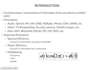
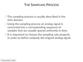
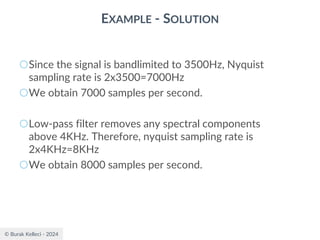
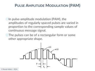
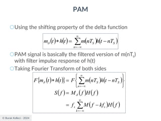
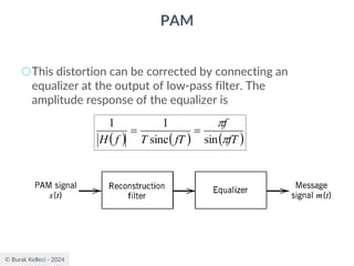
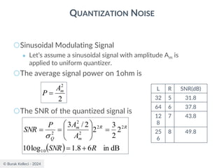
The document discusses digital communication and pulse amplitude modulation (PAM). It defines communication as the transmission of information from one point to another. Digital communication involves sampling analog signals, transmitting as a digital signal, and reconstructing at the receiver. PAM encodes information by varying the amplitude of uniformly-spaced pulses based on signal samples. The document provides illustrations of PAM encoding and discusses the important sampling rate requirement to avoid aliasing.


![© Burak Kelleci - 2024
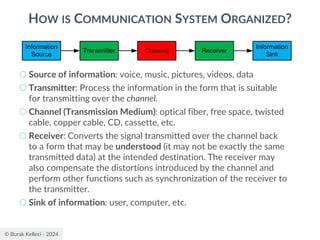
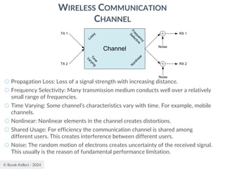
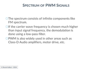
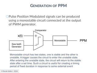
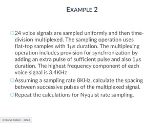
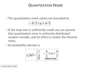
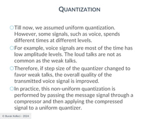
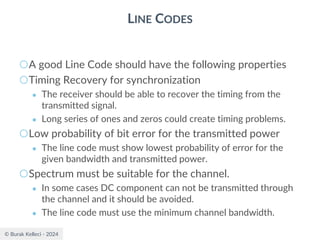
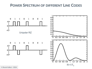
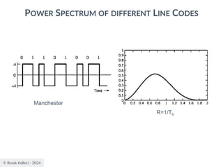
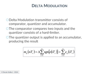
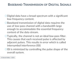
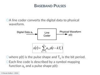
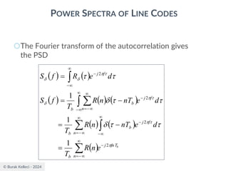
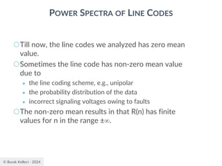
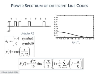
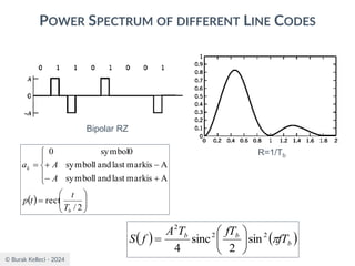
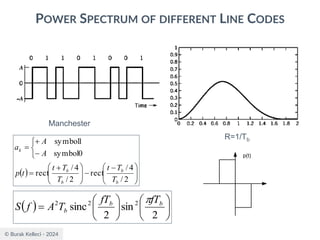
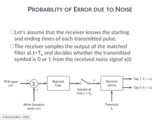
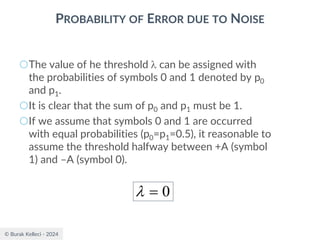
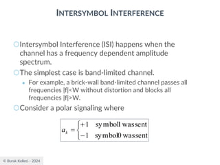
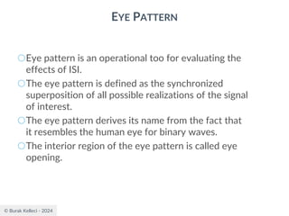
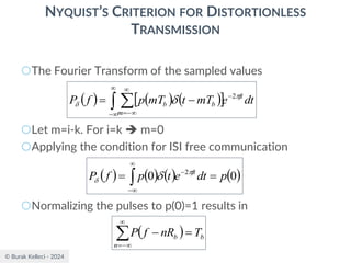
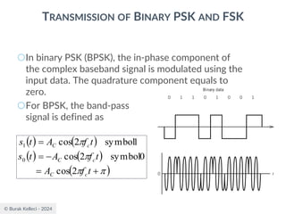
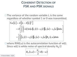
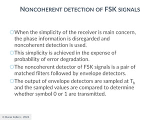
POWER SPECTRA OF LINE CODES
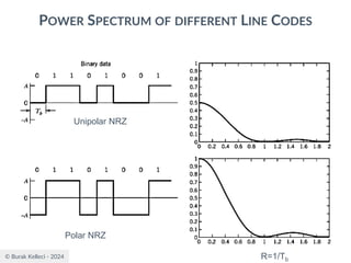
○For polar binary,
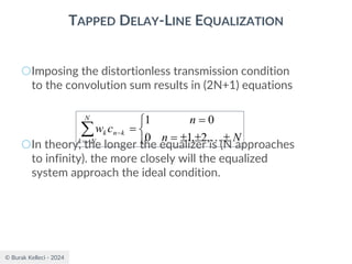
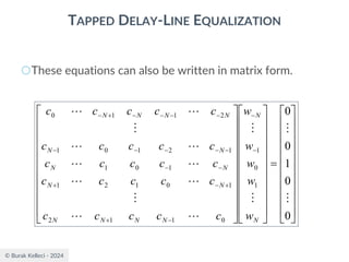
○n=0
● ak=ak+n = -A for symbol 0 and +A for symbol 1
● probabilities are p0=p1=0.5
● R(0)=(-A*-A)*0.5+(A*A)*0.5=A2
○n0
● [akak+n ]=[-A*-A], [-A*A],[A*-A], [A*A]
● p00=0.25, p01=0.25, p10=0.25, p11=0.25
● R(n0)=0
( ) ( ) ( ) ( )
b
b
n
b T
A
fnT
n
R
R
T
f
S
2
1
2
cos
2
0
1
=
+
=
=
](https://image.slidesharecdn.com/digitalcommunication-240222045408-77188038/85/Digital-Communication-fundamentals-pdf-134-320.jpg)
![© Burak Kelleci - 2024
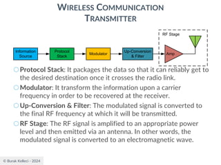
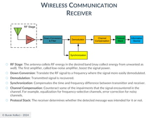
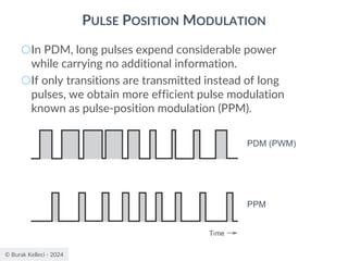
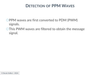
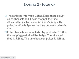
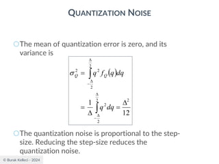
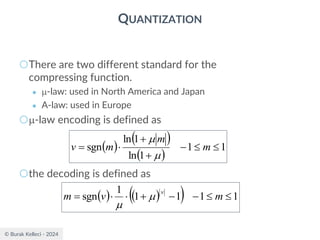
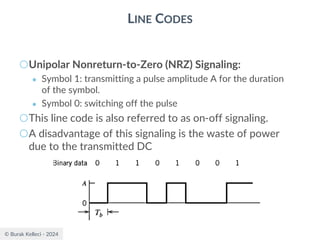
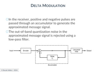
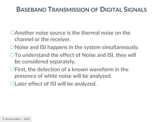
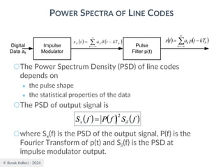
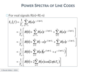
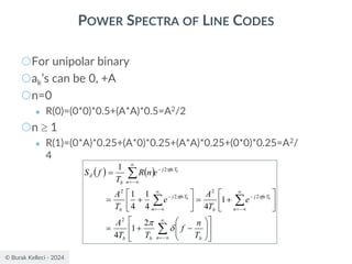
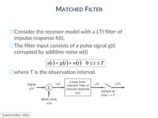
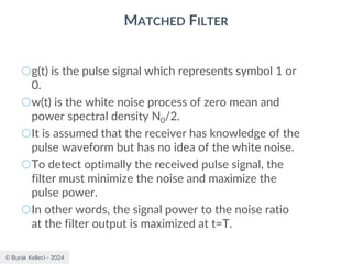
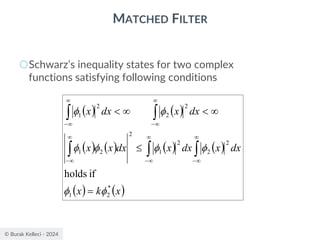
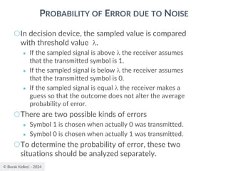
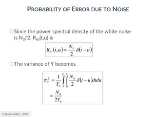
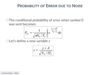
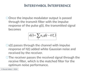
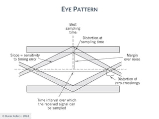
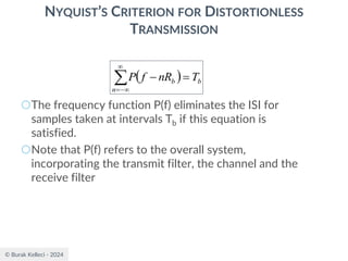
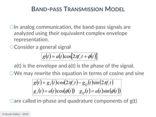
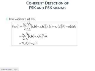
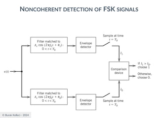
MATCHED FILTER
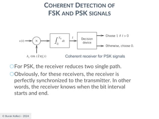
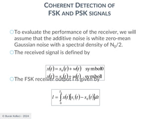
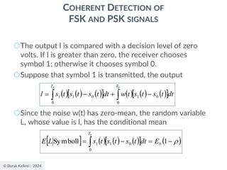
○Since the filter is an LTI system, the filter output
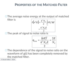
○The signal to noise ratio at the filter output
where |g0(T)|2 is the instantaneous power of the
output signal and E is the statistical expectation
operator, E[n2(t)] is the average output noise power.
○For optimum performance this ration is maximized.
( ) ( ) ( )
t
n
t
g
t
y +
= 0
( )
( )
t
n
E
T
g
2
2
0
=
](https://image.slidesharecdn.com/digitalcommunication-240222045408-77188038/85/Digital-Communication-fundamentals-pdf-145-320.jpg)
![© Burak Kelleci - 2024
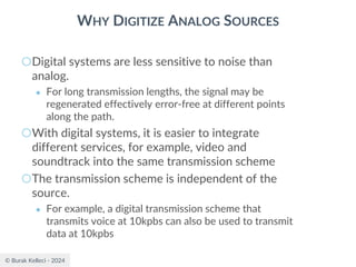
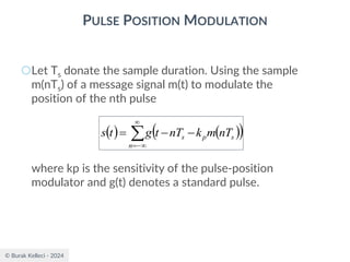
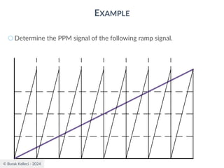
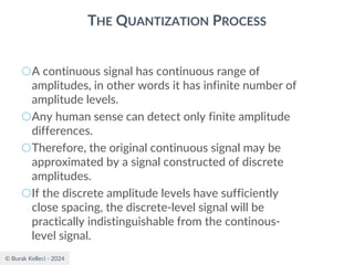
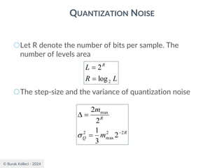
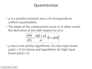
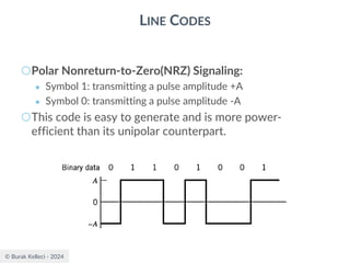
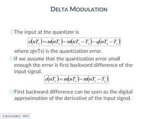
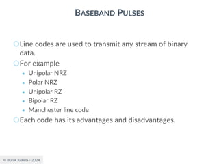
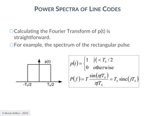
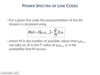
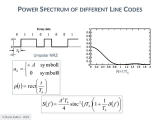
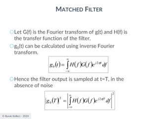
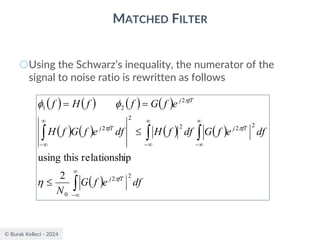
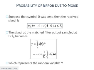
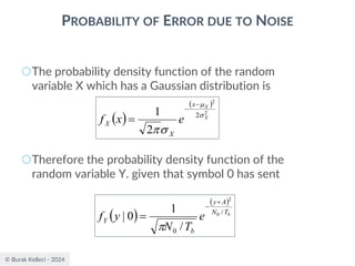
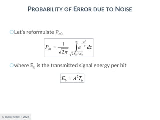
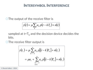
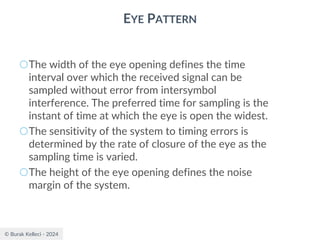
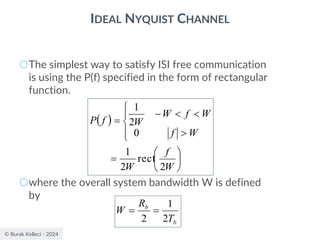
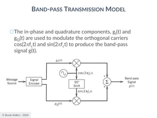
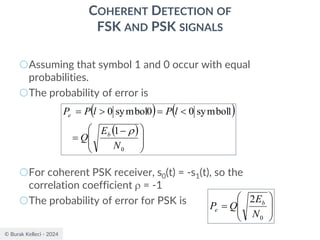
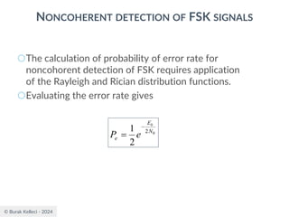
MATCHED FILTER
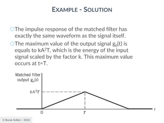
○Assuming g(t) is real [G*(f)=G(f)], the impulse
response of the filter is
○The impulse response of the optimum filter is
scaled, time-reversed and delayed version of the
input signal g(t).
( ) ( ) ( )
( ) ( )
( )
t
T
kg
df
e
f
G
k
df
e
f
G
k
t
h
t
T
f
j
t
T
f
j
opt
−
=
−
=
=
−
−
−
−
−
−
2
2
*](https://image.slidesharecdn.com/digitalcommunication-240222045408-77188038/85/Digital-Communication-fundamentals-pdf-152-320.jpg)
![© Burak Kelleci - 2024
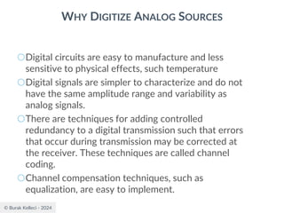
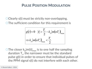
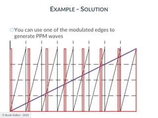
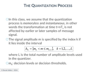
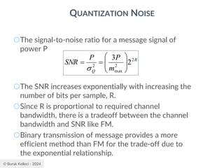
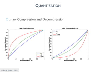
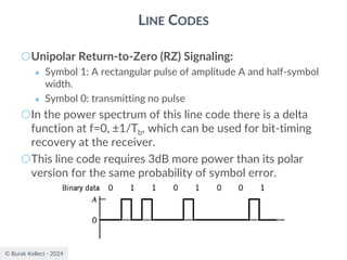
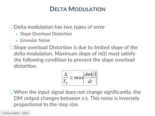
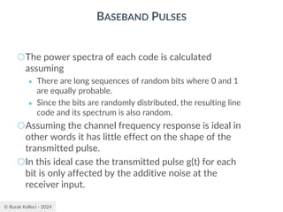
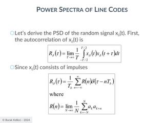
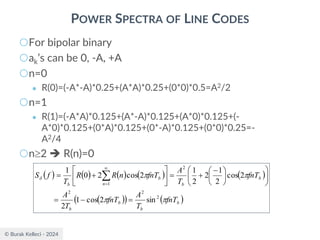
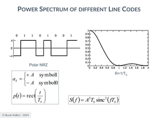
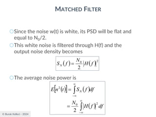
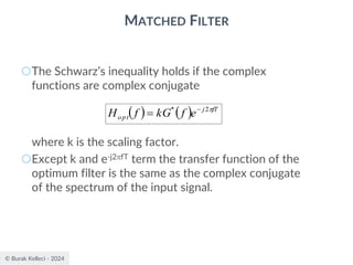
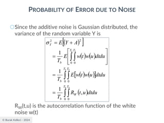
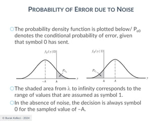
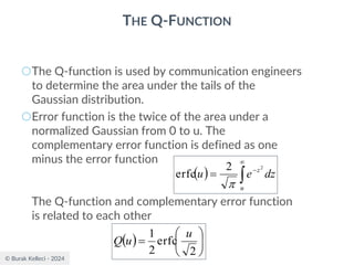
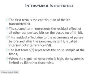
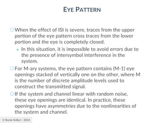
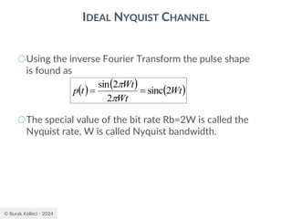
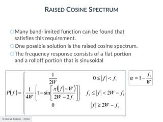
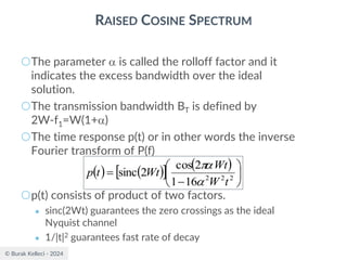
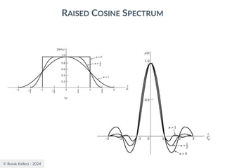
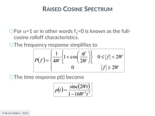
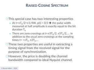
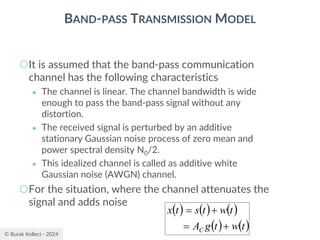
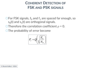
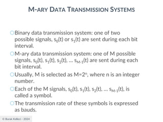
RAISED COSINE SPECTRUM
○The practical difficulties of the ideal Nyquist channel
is mitigated by extending the channel bandwidth
from the minimum value W to be adjustable
between W and 2W.
○Let’s keep three terms of
and restrict the frequency band of interest to
[-W,W]
( ) W
T
nR
f
P b
n
b 2
=
=
−
−
=
( ) ( ) ( ) W
f
W
W
W
f
P
W
f
P
f
P
−
=
+
+
−
+
2
1
2
2](https://image.slidesharecdn.com/digitalcommunication-240222045408-77188038/85/Digital-Communication-fundamentals-pdf-198-320.jpg)
![© Burak Kelleci - 2024
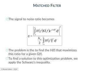
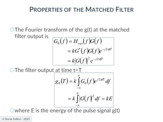
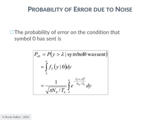
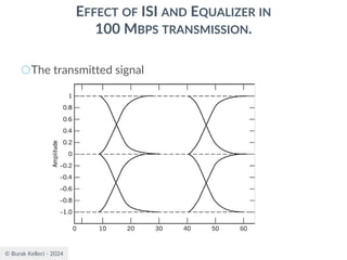
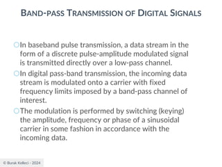
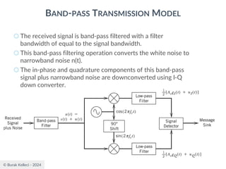
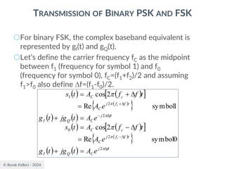
BAND-PASS TRANSMISSION MODEL
○The receiver will observe the complex representation of the
received signal [gI(t)+nI(t)]+j[gQ(t)+nQ(t)] for a duration of T
seconds and make the best estimate of the corresponding
transmitted signal gI(t)+jgQ(t) or equivalently the data symbol
0 or 1 for binary data.
○The hardware shown previous slide may be simplified
depending on the transmission strategy.
● Some methods use only in-phase signaling, so the quadrature path can
be removed.
● A noncoherent receiver recovers the symbols directly from the band-
pass signal without deriving in-phase and quadrature components.
● In modern receivers, the in-phase and quadrature oscillators are not
phase locked to the transmitter. This creates a phase rotation or even
a small frequency error. These problems are corrected by digital signal
processing algorithms.](https://image.slidesharecdn.com/digitalcommunication-240222045408-77188038/85/Digital-Communication-fundamentals-pdf-228-320.jpg)
![© Burak Kelleci - 2024
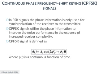
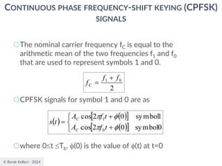
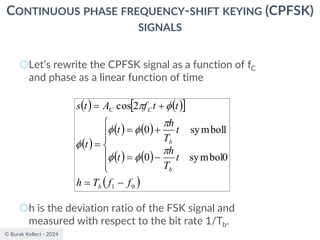
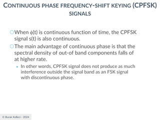
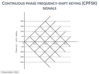
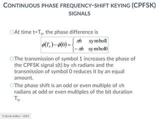
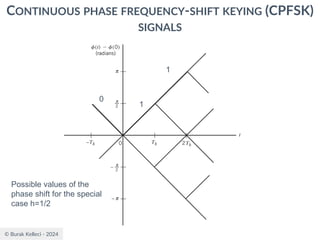
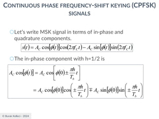
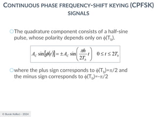
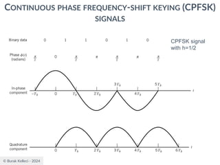
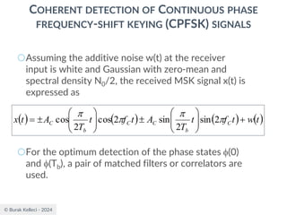
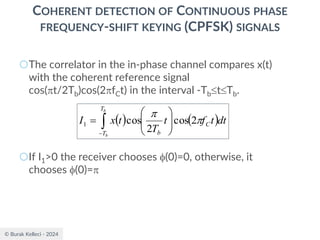
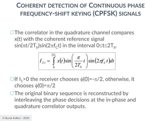
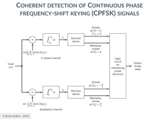
CONTINUOUS PHASE FREQUENCY-SHIFT KEYING (CPFSK)
SIGNALS
○Since (0) is 0 or depending on the past history of
the modulation process, the polarity of cos[(t)]
depends only upon (0).
○The in-phase component becomes
○where plus sign corresponds to (0)=0 and minus
sign corresponds to (0)=.
( )
b
b
b
C
C T
t
T
t
T
A
t
A
−
=
2
cos
cos
](https://image.slidesharecdn.com/digitalcommunication-240222045408-77188038/85/Digital-Communication-fundamentals-pdf-253-320.jpg)


![Multiband Transceivers - [Chapter 7] Multi-mode/Multi-band GSM/GPRS/TDMA/AMP...](https://cdn.slidesharecdn.com/ss_thumbnails/ch7-150613070936-lva1-app6892-thumbnail.jpg?width=640&height=640&fit=bounds)