This document summarizes a time series analysis of sunspot data from 1750 to 1950:
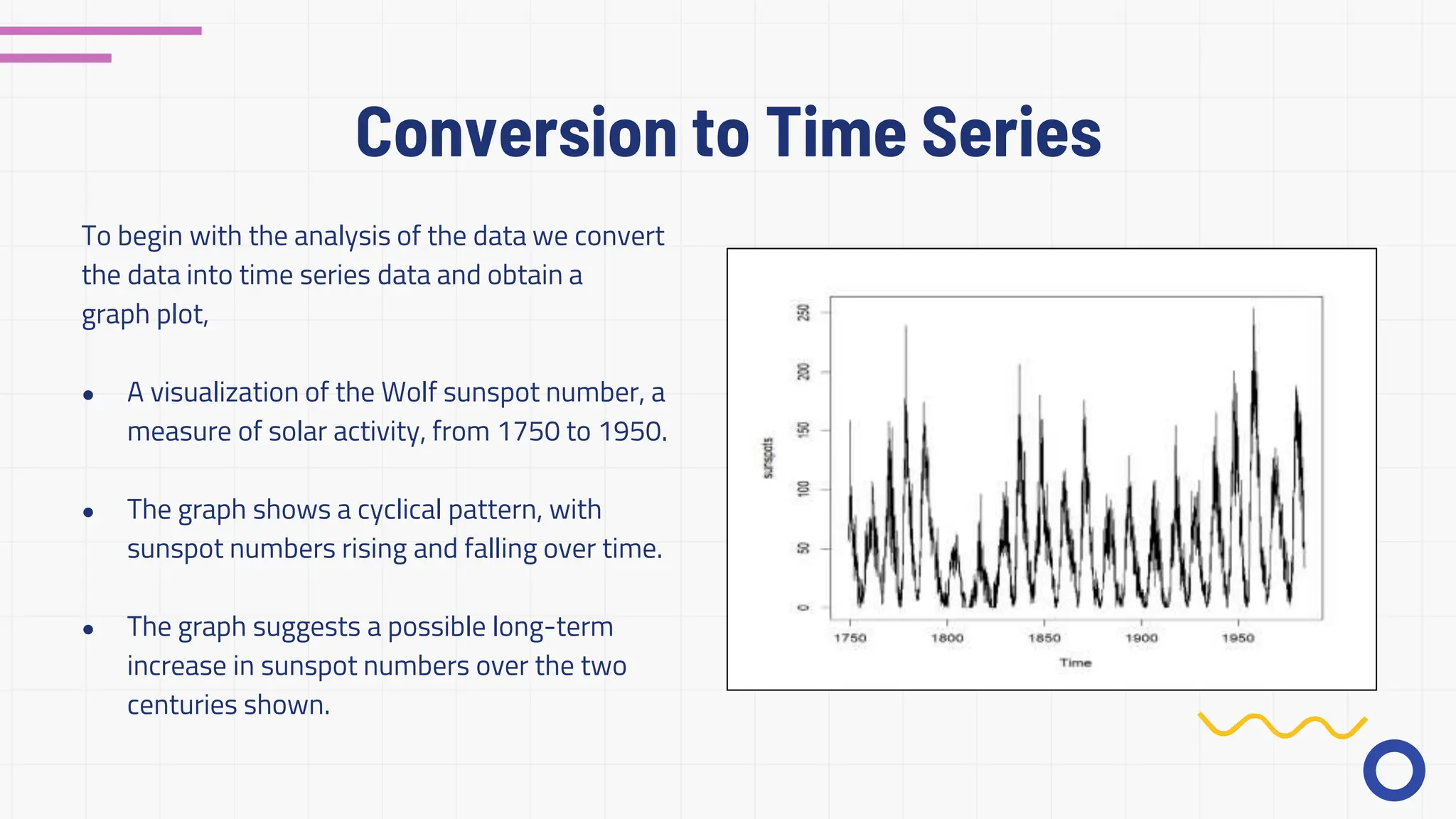
1. The analysis converted the sunspot data into a time series and found a cyclical pattern with sunspot numbers rising and falling over time, suggesting a long-term increase over the two centuries.
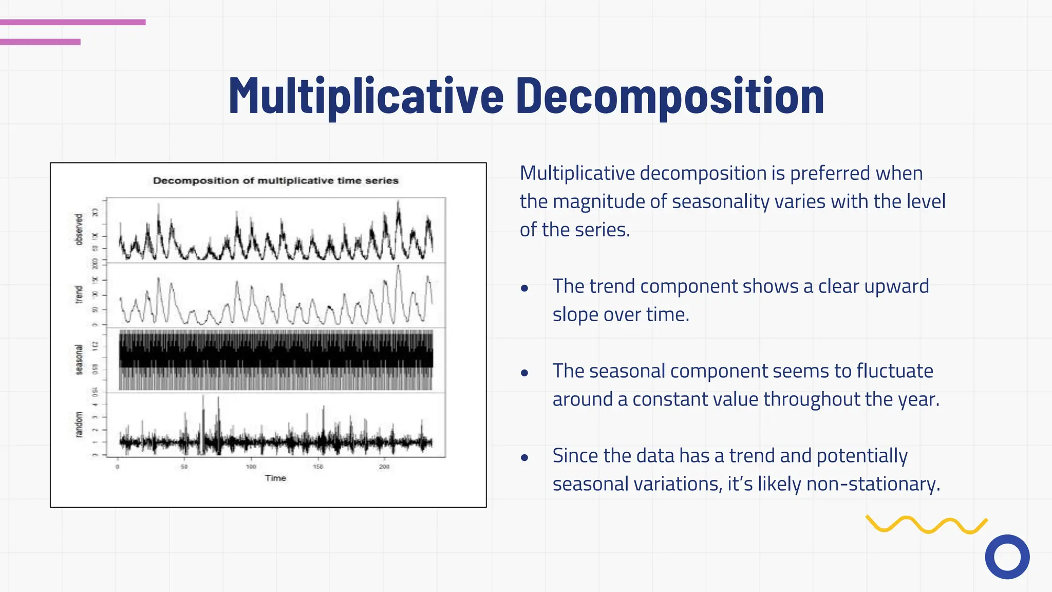
2. Using multiplicative decomposition, the analysis found the data had a clear upward trend over time along with potential seasonal variations, indicating it was non-stationary.
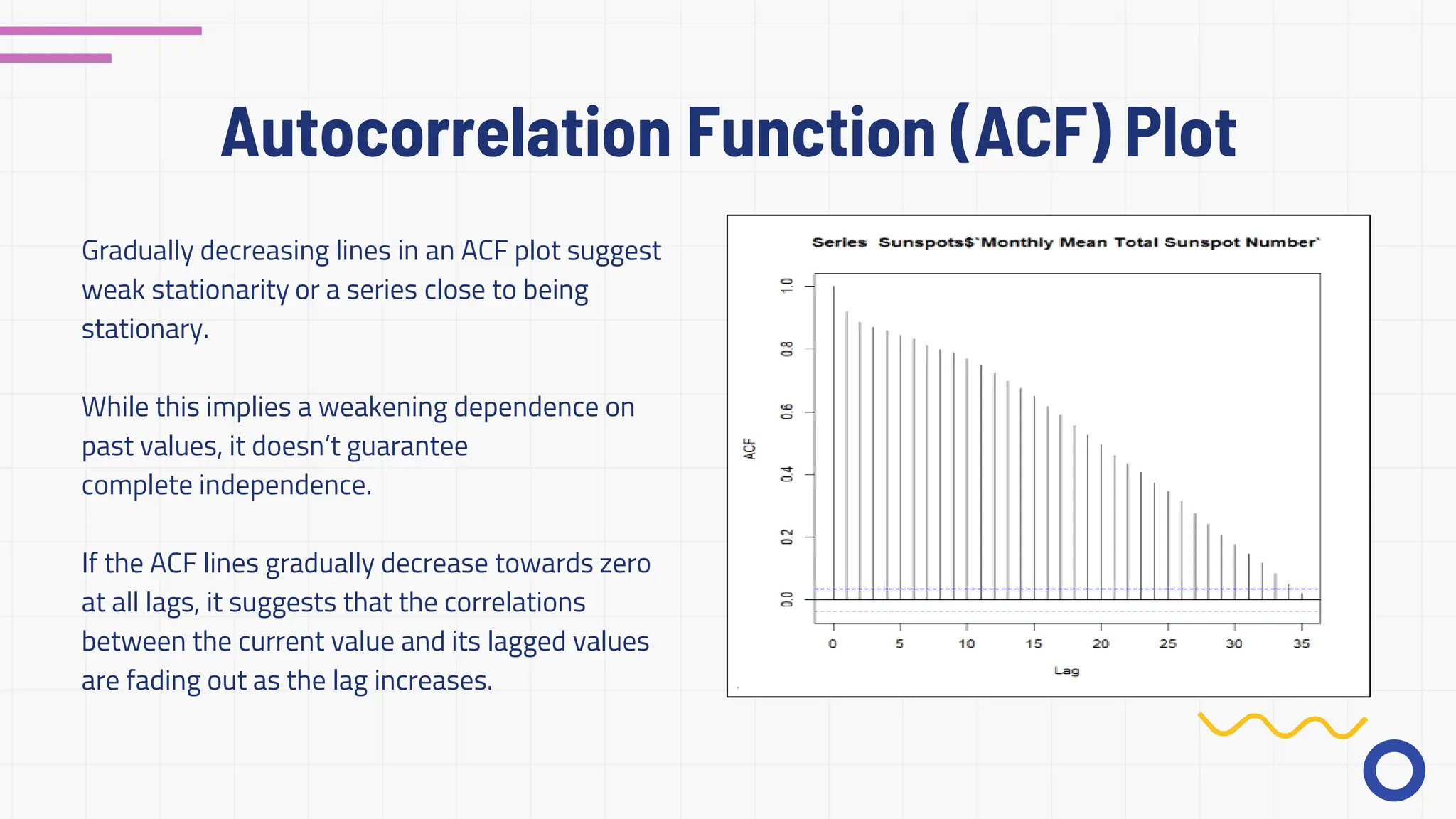
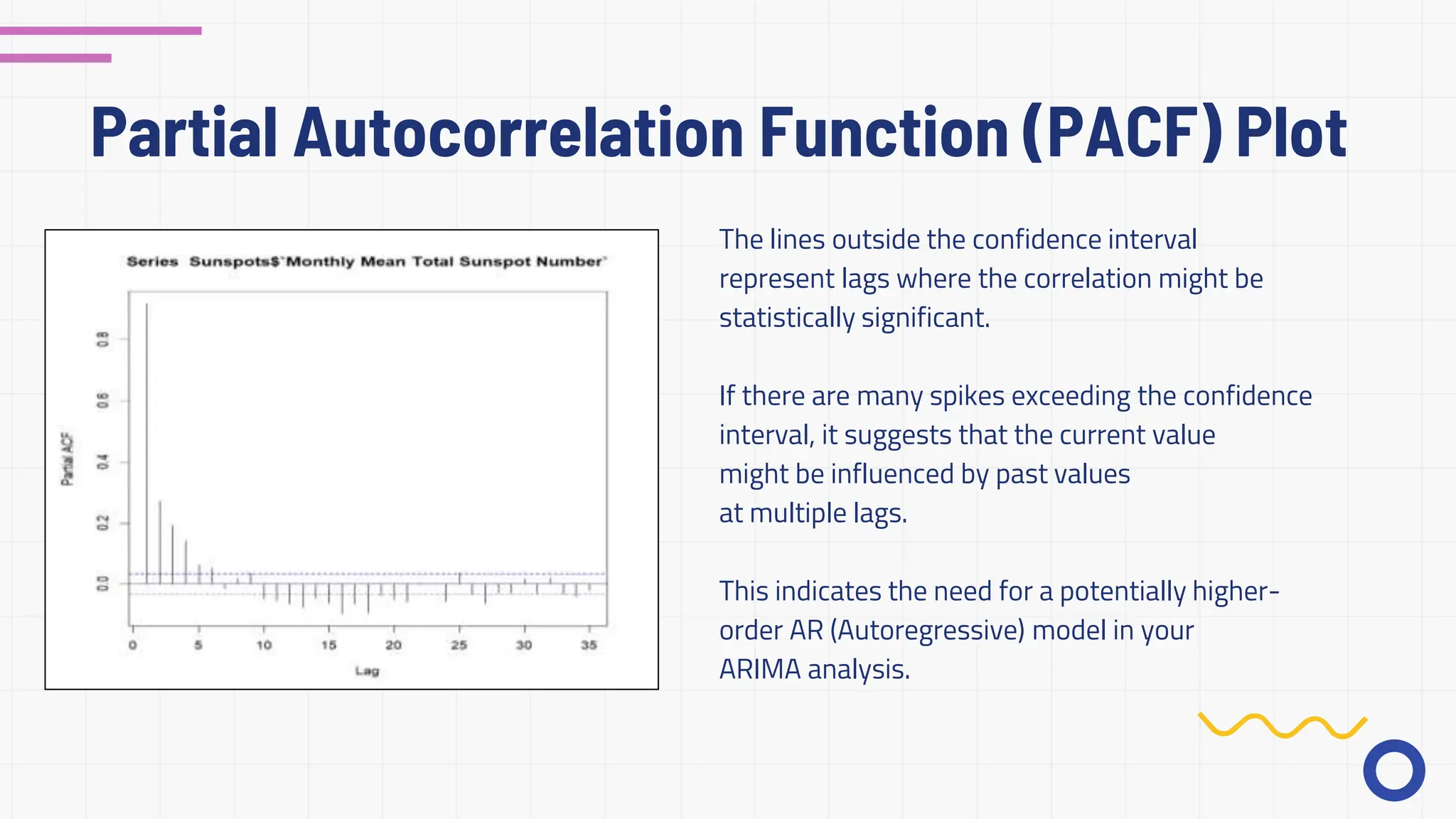
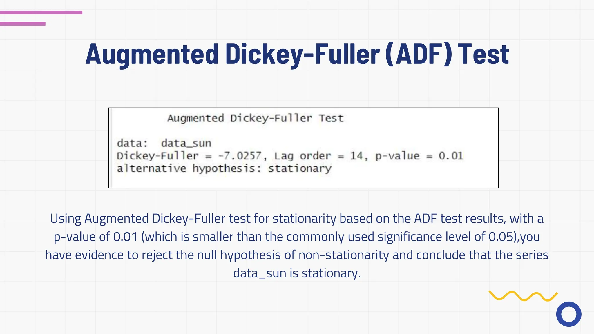
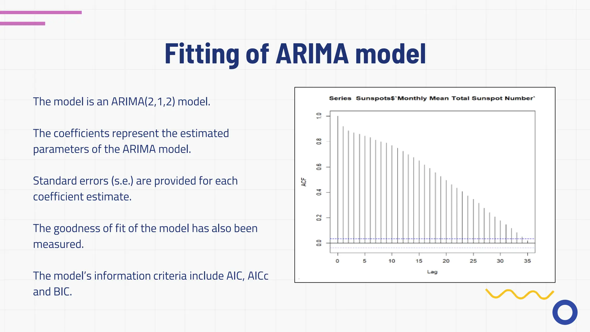
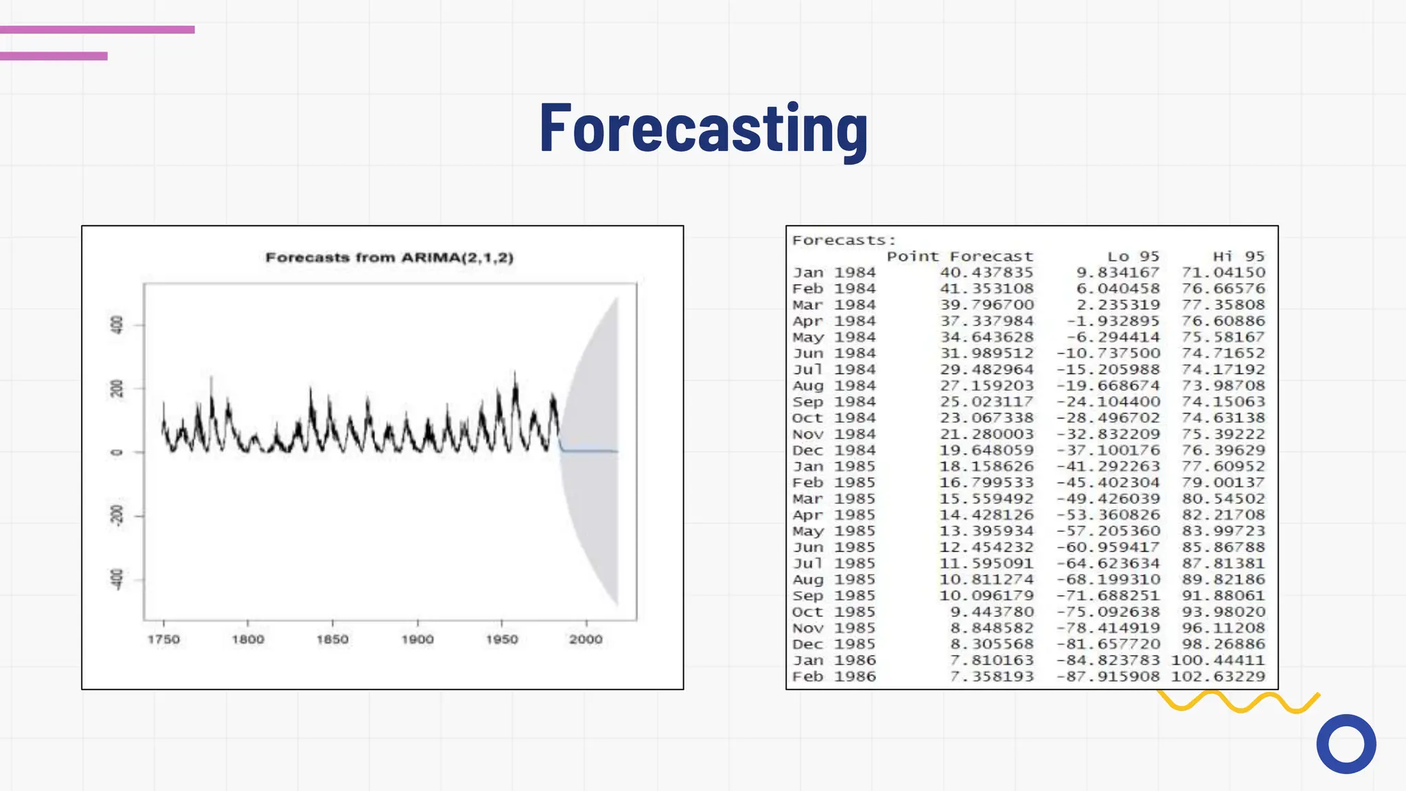
3. Autocorrelation and partial autocorrelation plots implied weak stationarity and multiple lag influences that suggested an ARIMA model. Testing confirmed the data was stationary. The best-fitting ARIMA(2,1,2)