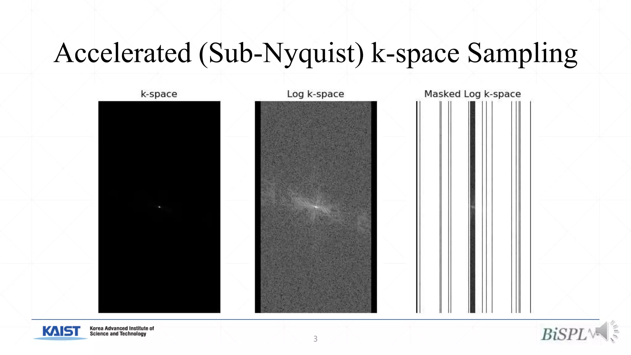
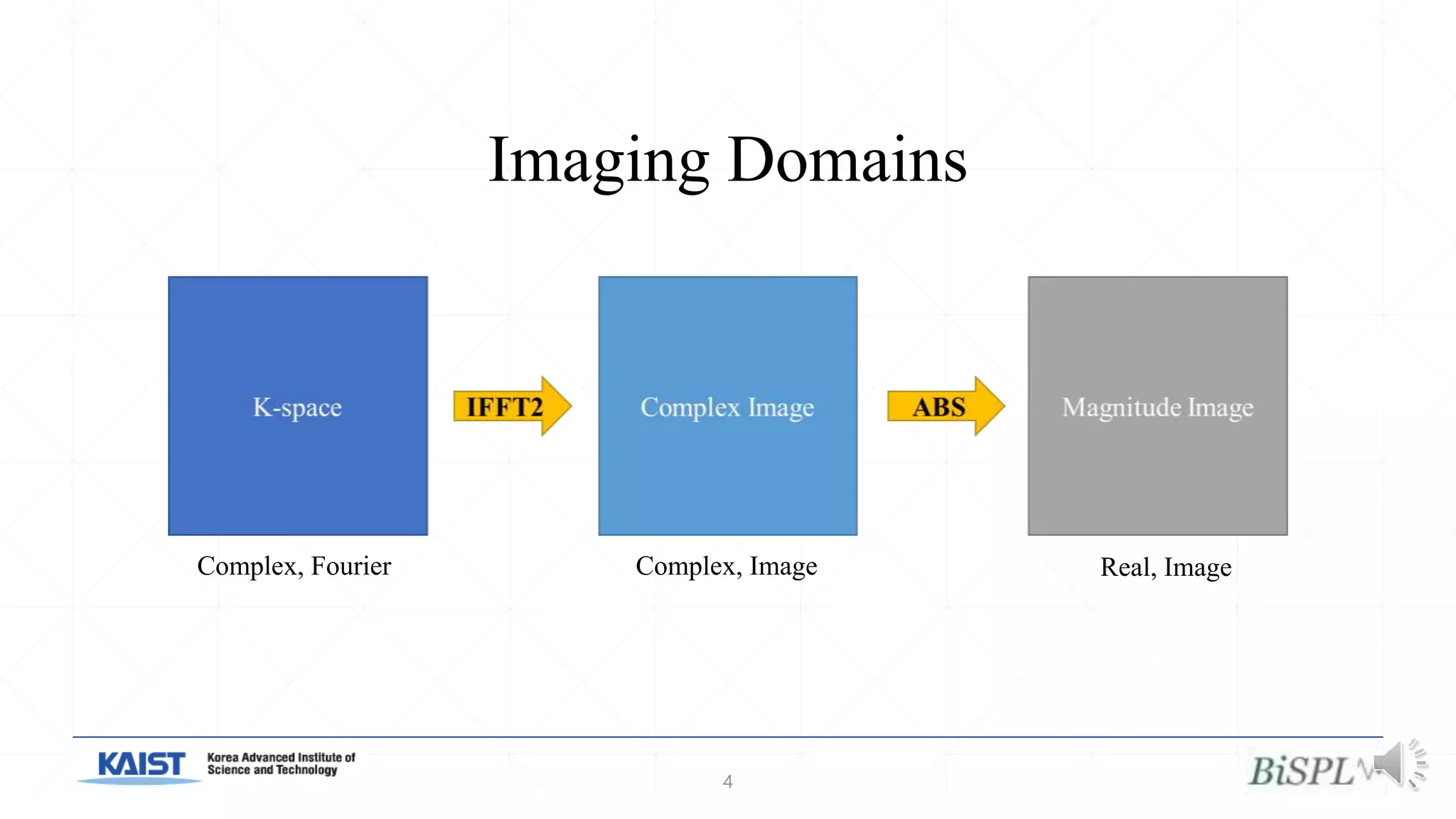
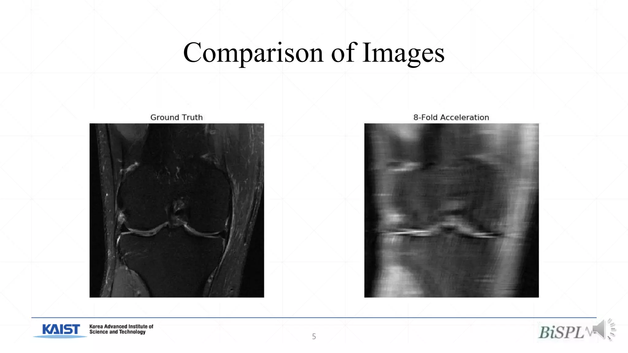
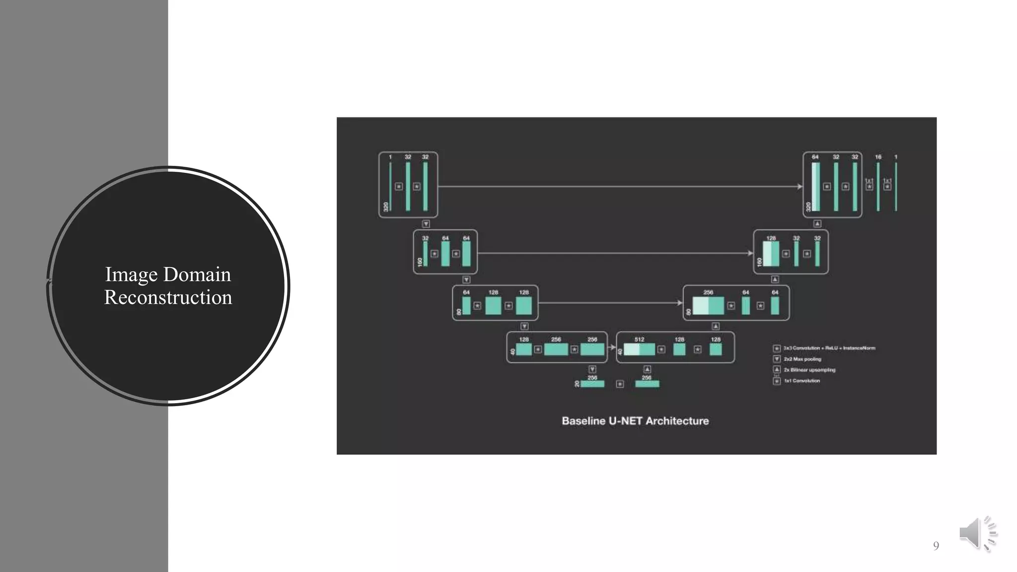
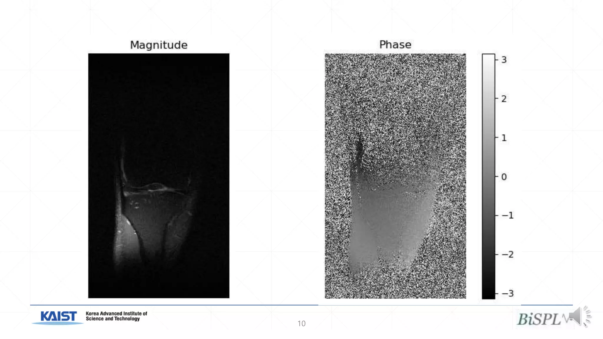
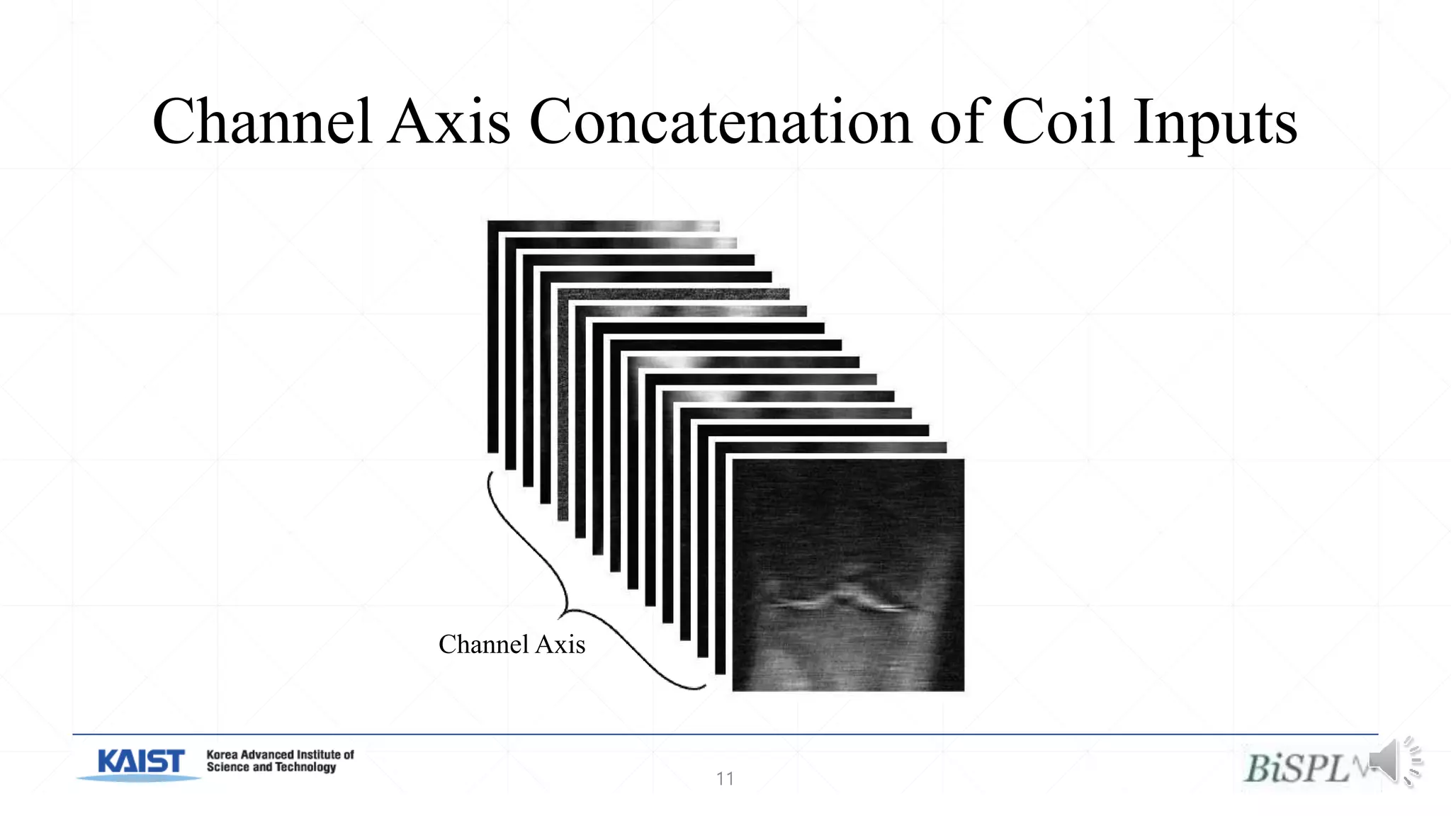
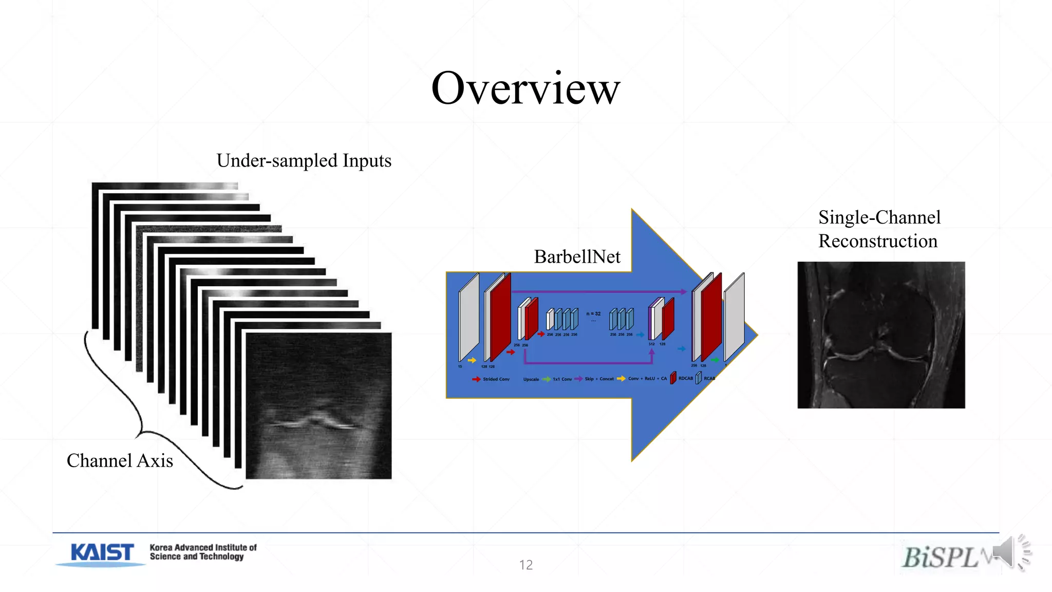
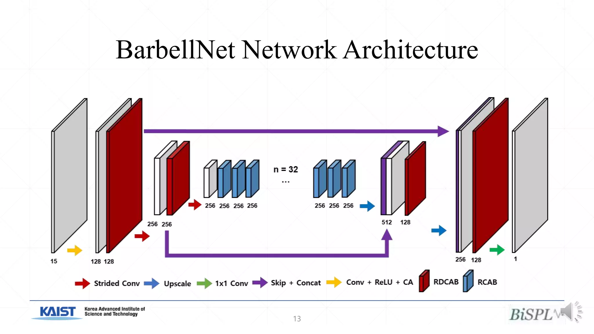
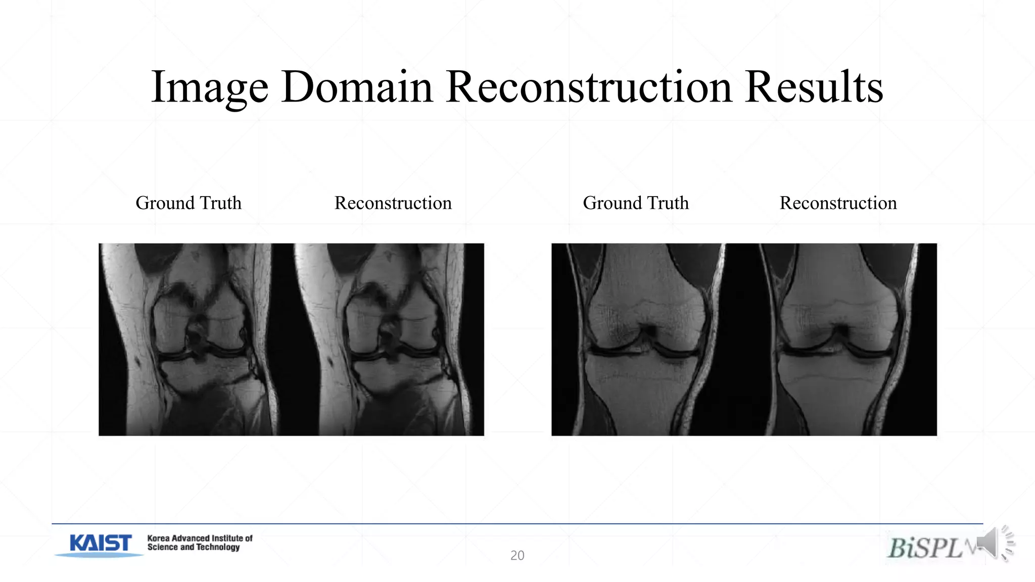
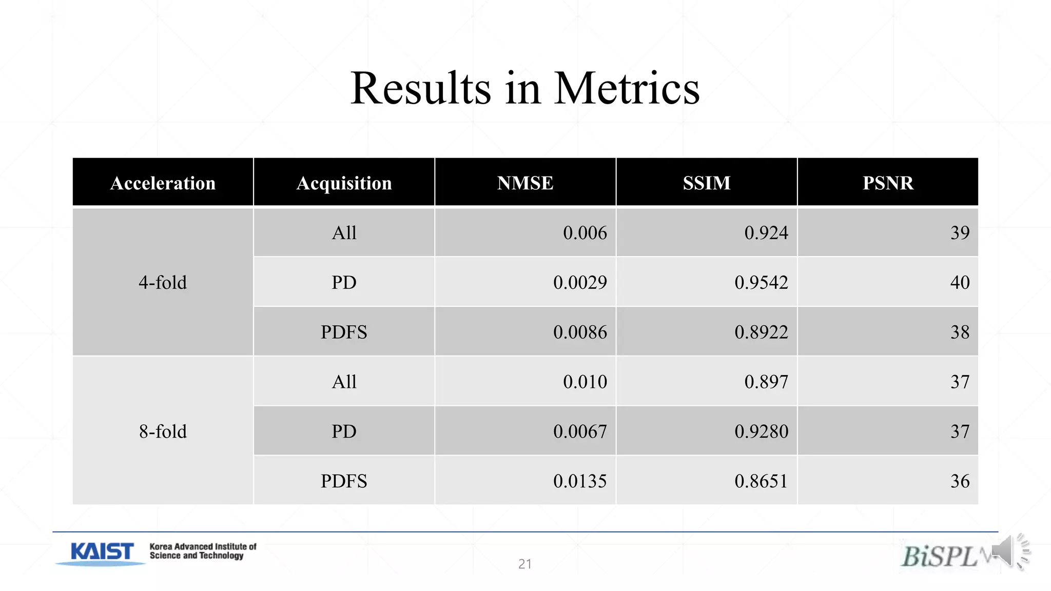
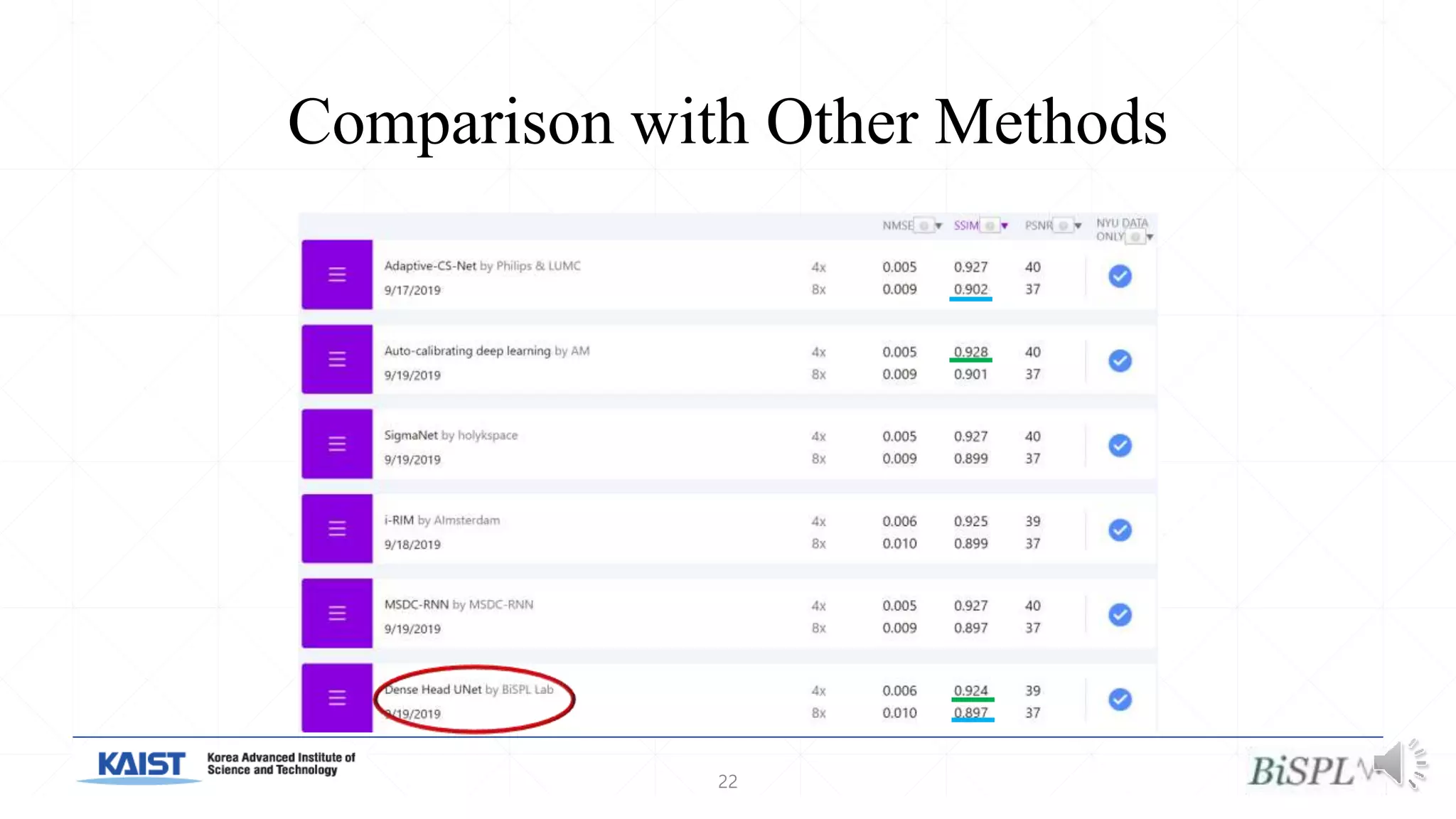
My presentation on how we participated in the fastMRI Challanege in 2019.
Aside from theoretical considerations, it also explains key implementation issues that arise in all deep learning for MRI such as disk I/O and CPU/GPU load balancing.
Used for presentation at ISBI 2020 Oral session.
Accidentally wrote the title as "Deep Learning Sum-of-Squares Images in Accelerated Parallel MRI". Sorry for the mistake!
6. Theoretical Challenges
• The raw k-space data lies in the signal domain, not the image domain.
• The k-space data consists of complex values, not real values.
• MRI machines have many coils to provide redundancy and reduce noise.
• It is not clear how to handle the multiple coils with different sensitivities.
6
8. Solutions to Theoretical Challenges
• Concatenate the coils in the channel axis.
• Use real-valued magnitude images as input, discarding image phase.
• Output a single channel with all coil information (no sum-of-squares).
8
14. Model Training Details
• 𝑺𝑺𝑰𝑴 𝟕 as loss function.
• Inputs center cropped to 320x320.
• Adam optimizer with 𝛽1 = 0.9, 𝛽2 = 0.999.
• Initial learning rate of 10−4, eventually reduced to 10−6 during training.
• Single GTX 1080Ti/2080Ti GPU used for training of ~100 epochs.
14
16. Practical Challenges
• Approximately 60% of teams could not manage implementation issues.
• Naïve data ETL pipeline has <10% GPU utilization.
• Disk I/O is a bottleneck due to the large size of multi-coil k-space data.
• CPU/GPU load balancing is a bottleneck for pre/post-processing of data.
16
18. Implementation Tips
• Compress the raw k-space data (HDF5 has native compression functionality).
• Store the data in fast SSD devices. SSDs also support parallel reads, unlike HDDs.
• Perform FFT (which is compute-heavy and parallelizable) on GPU, not CPU.
• Perform disk reading and host-to-device data transfer asynchronously and overlap
them with GPU computation.
18
23. Thank You for Listening!
• Code for this project is available at
https://github.com/veritas9872/fastMRI-kspace.
• The slides for this presentation are available at
https://www.slideshare.net/ssuserc416e2/presentations.
• Please contact the authors if you have any questions.
23
Editor's Notes
Hello, ISBI 2020. My name is Joonhyung Lee and today, I will introduce our work on MRI acceleration, which was done during our participation in the 2019 fastMRI Challenge.
I will begin with a brief introduction into the problems that we face.
Magnetic Resonance Imaging, or MRI, works by acquiring radio-frequency signals in the Fourier Domain. This information is set in a grid known as k-space. According to the Nyquist Sampling Theorem, a signal must be sampled at at least double the maximum frequency to produce a sound analog representation. However, MRI scans take a long time and a major research goal in MRI is to reduce scanning times.
Because most of the information in an image is concentrated in the low frequency region at the center of k-space, we can reduce the amount of sampling in higher frequency regions while retaining most of the information. We can thus reduce the acquisition time significantly with minimal loss of information. The image on the right shows an 8-fold acceleration with 4% sampled at the low frequency ACS region.
After acquiring the k-space signal, the inverse Fourier Transform is applied to create an image of the underlying object. This image will be a complex-valued image. We create a real-valued image from the magnitude values of this complex-valued image. Also, modern MRI machines have multiple radio-frequency coils, which create separate images with different sensitivities to different locations. A single image is formed by performing a root-sum-of-squares on the magnitude image of each coil.
As you can see from the knee images, even with 8-fold acceleration of the high frequency regions, the general outline of the underlying object is still visible.
However, we wish to reconstruct an image suitable for use in medical diagnosis. To this end, we use deep learning produce a high-quality image from the information latent within the under-sampled data.
However, due to the unique nature of MRI, several theoretical challenges arise that need to be solved.
First, k-space data lies in the signal domain, where each point contains information about the entire image.
Second, k-space consists of complex numbers, whereas almost all deep learning models use real numbers.
Third, modern MRI machines have multiple radio-frequency coils, each with different sensitivities to different locations.
Moreover, the number of coils and the location of each coil is different for each device.
In the following section, I will discuss our solutions to these problems.
After much experimentation, we arrived at the following solutions.
First, we concatenate the coils in the channel axis.
Second, we used the magnitude images for each coil as the input.
Finally, we found that outputting a single-channel image for the final reconstruction produced much superior results than producing results for each coil separately.
Image domain reconstruction is the form used by the vast majority of deep learning image reconstruction models.
Over the last few years, through extensive experimentation, it has been proven to work on a wide array of images.
While this discards the complex-image phase information, this solved the problem of handling complex numbers.
Image domain learning for MRI loses the phase information of the complex-valued image.
The images above show the magnitude and phase from a single coil in a slice in an MRI scan.
While this means that the images cannot be converted back into k-space, for k-space input consistency, we find that the magnitude images contain enough information to allow high quality reconstruction.
Concatenating the coils in the channel axis allows the model to utilize the information from each coil while dramatically reducing the amount of computation compared to other methods. For example, concatenation in the batch axis would have entailed a 15-fold increase in memory and computation time on the fastMRI dataset. Also, the different coil sensitivities are available to the entire model all the time.
One limitation is that this requires all data to have the same number of coils, each with the same sensitivity information.
Channel concatenation was possible on the fastMRI knee dataset because it consists entirely of MRI scans with 15 coils.
Finally, we take the magnitude images from each coil and, instead of performing a root-sum-of-squares operation, input the coil images into a neural network.
The output is a single image that is compared to the ground-truth root-sum-of-squares image.
This method produces better results than separate generation of coil images.
We suspect that this is because this allows the model to learn the best method to combine the coil information.
Our model is loosely based on the U-Net architecture but has a long chain of residual channel attention blocks, or RCABs, in the middle and multiple DenseBlocks for efficient feature extraction. The residual blocks were based on the EDSR residual block, which is optimized for image reconstruction.
No feature normalization layers were included in the model to reduce computation and improve metric performance by preserving the original distribution and allowing for greater representational capacity of the model.
The channel attention mechanism is identical to the Squeeze Excitation channel attention mechanism. Channel attention of this type has been shown to be very effective for both high-level tasks such as classification as well as low-level image denoising and super-resolution. We also found that it helped stabilize network training, which was very important because the lack of normalization layers caused training instability.
We termed our model “BarbellNet” due to its resemblance to a barbell.
During training, we used structural similarity (SSIM) with kernel size 7 as the sole loss function as this was the primary metric of the fastMRI challenge.
Inputs were center cropped to 320x320 to reduce computation and create a uniform input size.
Learning rate decay was used to reduce the learning rate from 10^-4 to 10^-6.
Finally, all models were trained on a single GTX 1080Ti or RTX 2080Ti GPU.
These hardware requirements are within the reach of most researchers.
Finally, I would like to mention some challenges in implementation.
The unique nature of k-space data poses not only theoretical challenges but also practical challenges in implementation that mean that standard deep learning pipelines are very inefficient. A naïve data pipeline will significantly under-utilize GPU, but the causes of this under-utilization will not be obvious. Because of this, approximately 60% of challenge contestants could not participate in the multi-coil challenge but only applied to the single-coil track, which consists of synthetic data derived from the multi-coil raw data.
The biggest problem is the very large size of each MRI slice or volume. Reading data from HDD is very slow. This means that the CPU and GPU are idle most of the time, waiting for data to arrive.
The second issue is data pre-processing. The Fourier Transform is very computationally intensive and performing it on CPU on such a large amount of data will form a bottleneck, no matter how efficiently implemented.
To solve these problems, we offer these solutions.
First, to solve the problem of disk I/O, the simplest solution is to use an SSD storage device to store the data. Additionally, you can compress the data file to reduce the amount of raw data that must be read from disk, although this comes at the cost of increased CPU computation.
Second, perform Fourier Transforms on GPU, not CPU. There are many highly optimized Fourier Transform libraries on GPU.
Finally, overlap disk reading on multiple processes and overlap it with GPU computation. This will prevent the GPU from being idle for too long.
Finally, our results.
We have here a qualitative comparison between the ground truth and reconstruction images.
Compared to the inputs, they are much clearer and show no obvious artifacts.
One limitation is that there is a loss of detail in the horizontal direction, the direction of down-sampling.
The chart shows our results in more quantitative form. One can see that different accelerations and different acquisition methods have very different average metrics. 4-fold acceleration with 8% ACS sampling has superior results compared to 8-fold acceleration with 4% ACS sampling because the former has more signal in the input data.
PD, or Proton Density images have better metrics than PDFS, or Proton Density Fat Suppression because the fat suppression acquisition sequence increases the amount of noise, although it also reduces the visibility of fat.
Our methods were very close to competitors in terms of metrics. Even compared to the first-place results, there was only a small difference in SSIM. Our results are therefore comparable to even state-of-the art methods, despite using fewer computational resources.
This is the end of the session. Thank you for listening. Please contact us if you have any questions and have a good day.