This document presents two theoretical models of determinants of informality and tests their implications using survey data from over 50,000 small firms in Brazil. The first model finds that informal firms face higher capital costs and size limitations, resulting in smaller size and lower capital-labor ratios compared to formal firms. The second model highlights how value-added taxes can transmit informality between firms in a supply chain. Empirical analysis supports the models' implications and finds measures of supplier and purchaser formality are correlated with a firm's own formality, especially in sectors subject to value-added tax credits.

1. The Informal Sector
´Aureo de Paula †
University of Pennsylvania
Jos´e A. Scheinkman ‡
Princeton University and NBER
First version: January 11, 2006
This Version: July 12, 2006
We thank Rita Almeida and Sandra Brand˜ao for their help with the enforcement data, Joana
Monteiro and Juliano Assun¸c˜ao for providing the ECINF dataset and for clarifying its content and
methodology, and Julio Cacho for research assistance. We also benefited from comments by seminar
participants at the 2006 NASMES. Scheinkman’s research was supported by the National Science
Foundation through grant 0350770.
†Department of Economics, University of Pennsylvania, Philadelphia, PA 19104. E-mail:
aureo@sas.upenn.edu
‡Department of Economics, Princeton University, Princeton, NJ 08544. E-mail:
joses@princeton.edu
1

2. Abstract
This paper investigates the determinants of informal economic activity. We present two equilibrium
models of the determinants of informality and test their implications using a survey of 50,000+
small firms in Brazil. We define informality as tax avoidance; firms in the informal sector avoid
tax payments but suffer other limitations. In the first model there is a single industry and informal
firms face a higher cost of capital and a limitation on size. As a result informal firms are smaller
and have a lower capital-labor ratio. These implications are supported by our empirical analysis.
A novel theoretical contribution in this paper is a model that highlights the role of value added
taxes in transmitting informality. It predicts that the informality of a firm is correlated to the
informality of firms from which it buys or sells. The model also implies that higher tolerance for
informal firms in one production stage increases tax avoidance in downstream and upstream sectors.
Empirical analysis shows that, in fact, various measures of formality of suppliers and purchasers
(and its enforcement) are correlated with the formality of a firm. Even more interestingly, when we
look at sectors where Brazilian firms are not subject to the credit system of value added tax, but
instead the value added tax is applied at some stage of production at a rate that is estimated by
the State, this chain effect vanishes.
JEL Codes:
2

3. 1 Introduction
In this paper we investigate the determinants of informality. It is difficult to unam-biguously
define informal activities but estimates indicate that in 1990-1993 around
10% of GDP in the United States was produced by individuals or firms that evaded
taxes or engaged in illegal pursuits. It is also estimated that these activities produce
25 to 35% of output in Latin America, between 13 to 70% in Asian countries, and
around 15% in O.E.C.D. countries. (see Table 2 in Schneider and Enste [17]).
Informality creates a fiscal problem, but there is also growing evidence that
informal firms are less efficient,1 perhaps because of their necessarily small scale,
perhaps because of their lack of access to credit or access to the infrastructure of legal
protection provided by the State. For less developed countries, creating incentives for
formalization is viewed as an important step to increase aggregate productivity.
We present two equilibrium models of the determinants of informality and
test their implications using a survey of 50,000+ small firms in Brazil. In both
models informality is defined as tax avoidance. Firms in the informal sector avoid
tax payments but suffer other limitations.
The first model can be seen as a variant of Rausch [14], who relied on the
modeling strategy of Lucas [11] in which managerial ability differs across agents in
the economy, and assumed a limitation on the size of informal firms. We make a key
modification that generates testable implications. The firms in our model use capital
in addition to labor and informal firms face a higher cost of funds. This higher cost
of capital for informal activities has been emphasized by DeSoto [4] who wrote that
“Even in the poorest countries, the poor save. The value of savings among the poor
is, in fact, immense − forty times all the foreign aid received throughout the world
since 1945. (. . . ) But they hold these resources in defective forms: houses built on
land whose ownership rights are not adequately recorded, unincorporated businesses
with undefined liability, industries located where financiers and investors cannot see
them. Because the rights of these possessions are not adequately documented, these
assets cannot readily be turned into capital, cannot be traded outside of narrow local
circles where people know and trust each other, cannot be used as collateral for a loan,
and cannot be used as a share against investment.”2 This difference in interest rates
1McKinsey [12] provides case study evidence on the impact of informality on firms’ productivity.
They estimate that the ratio of labor productivity between informal and formal firms is 39% in
Turkey and 46% in Brazil.
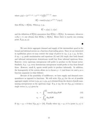
2DeSoto [4], p.5-6. DeSoto [3] estimates that in June/85, informal firms in Lima (Peru) faced a
nominal interest rate of 22% per-month, while formal firms paid only 4.9% per month. Straub [18]
3

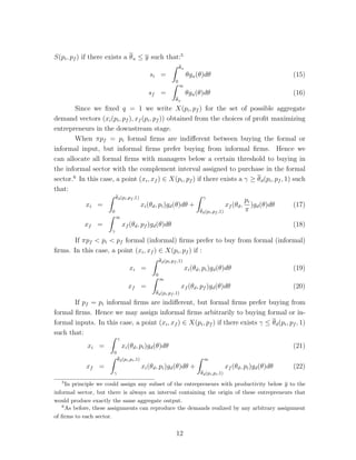
4. induces a higher capital-labor ratio in formal firms.3 As in Rausch [14], agents with
lowest managerial ability become workers and the ones with highest ability become
formal managers, with the intermediate group running informal firms. This is because
managers with more ability would naturally run larger firms and employ more capital;
for this reason they choose to join the formal sector, where they do not face limits on
capital deployment and face a lower cost of capital. The marginal firm trades off the
cost of paying taxes versus the higher cost of capital and scale limitations of informal
firms. As a result, the marginal firm would employ in the informal sector less capital
and labor than it would employ if it joined the formal sector. Thus, as in Rausch [14]
or Fortin et al. [6], a size gap develops. Managers that are slightly more efficient than
the manager of the marginal firm employ discretely larger amounts of capital and
labor.
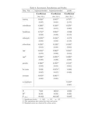
Several implications of this model are supported by our empirical analysis.
Formalization is positively correlated with the size of firms and measures of the qual-ity
of the entrepreneurial input. Even after controlling for our measures of the quality
of an entrepreneur, formalization is correlated with a firm’s capital-labor ratio or in-vestment
per worker. In addition, after controlling for the quality of the entrepreneur,
formalization is correlated with higher profits.
The main focus of our theoretical analysis is a model that highlights the role
of value added taxes in transmitting informality. The value added tax is a prevalent
form of indirect taxation: more than 120 nations had adopted it by 2000.4 It exploits
the idea that collecting value added taxes according to a credit scheme sets in motion
a mechanism for the transmission of informality. In the credit or invoice method the
value added tax applies to each sale and each establishment receives a credit for the
amount of tax paid in the previous stages of the production chain. This credit is then
used by the taxpayer against future liabilities with the tax authorities. The credit
method is often used in practice because it offers advantages over other collection
methods: (1) the tax liability is attached to the transaction and the invoice provides
an important documentary evidence; (2) an audit trail is established and there is an
important self-monitoring dimension across firms in different stages of the production
chain; (3) multiple rates can be used and certain activities may be exempt for social
or economic purposes (see [19]). Since purchases from informal suppliers are ineligible
for tax credits, an incentive exists for the propagation of informality downstream in
develops a model in which a dual credit system arises in equilibrium.
3It is also probable that informal firms face lower labor costs, because their workers avoid some
labor taxes. This would induce even larger differences in capital-labor ratio.
4See Appendix 4 in Schenk and Oldman [16].
4

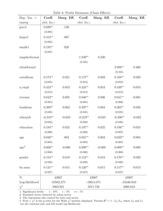
5. the production chain. A similar mechanism also influences firms upstream in the
chain: selling to informal firms increases the likelihood for a firm to be informal. Our
empirical analysis shows that, in fact, various measures of formality of suppliers and
(and its enforcement) purchasers are correlated with the formality of a firm. Even
more interestingly, when we look at sectors where Brazilian firms are not subject
to the credit system of value added tax, but instead the value added tax is applied
after some stage of production at a rate that is estimated by the State, this chain
effect vanishes. To our knowledge, the only study to investigate the informal sector
in conjunction with a VAT structure is Emran and Stiglitz [5]. Their focus is on the
consequences of informality for a revenue neutral tax reform involving value added
and trade taxes.
Our models ignore some possible alternative reasons for informality, such as the
fixed cost of complying with regulations or the existence of a minimum-wage. While
we could accommodate the existence of a minimum wage, some empirical evidence
actually points out that minimum wages may be as binding (if not more) in the
informal sector than in the formal segment of the economy in Latin America (see
Maloney and Mendez [13]).
Other papers that investigate causes and determinants of informality include
Loayza [10], Friedman et al. [7], and Junqueira and Monteiro [9] who used the same
dataset as we do. These authors have provided evidence of an association between
the size of the underground economy and higher taxes, more labor market restric-tions,
and poorer institutions (bureaucracy, corruption and legal environment). The
combination of the models we develop and the Brazilian microdata allows us to add
novel insights to this literature.
The remainder of this paper is organized as follows. In the next section we
develop a model of a single industry, while in Section 3 we treat the model with two
stages of production. Section 4 contains the empirical results obtained using data on
informal firms in Brazil and Section 5 concludes.
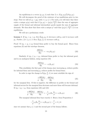
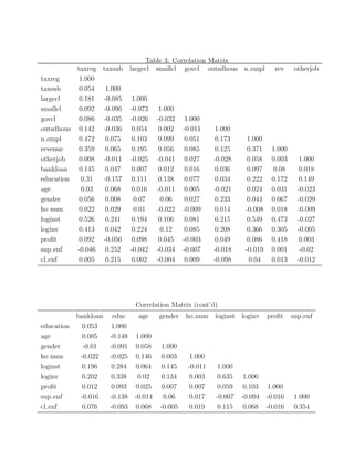
2 A Model with One Production Stage
We consider a continuum of agents; each characterized by a parameter 0 which
indicates his quality as an entrepreneur and is distributed according to a probability
density function g(·). An entrepreneur chooses between becoming a worker, operating
a firm in the formal sector or in the informal sector. If an entrepreneur employs l
workers and k units of capital, output equals y = kl

6. , with ,

7. 0 and +

8. 1.
5

9. A formal entrepreneur pays an ad valorem tax rate of and faces a capital
cost of rf 0 per unit. An informal entrepreneur pays no taxes, but faces a capital
cost of ri rf . All workers are paid the same wage w.
An informal entrepreneur, if detected by the authorities, loses all his profits.
The probability of being detected depends monotonically on the size of the firm.
Though there are several possibilities for measuring the size of the firm - output,
capital stock or labor force - we choose here the size of the capital stock (which we
identify in the empirical work as the value of installations), because we imagine the
probability of detection as a function of the “visibility” of the firm. We write p(k) for
the probability of detection. While in the appendix we discuss a more general form
for the function p we will assume here that:
p(k) = 0, if k k (1)
= 1, if k k, (2)
that is an informal firm cannot employ more than k units of capital, but will not
suffer any penalty when k k.
Hence the profit for an entrepreneur of quality that chooses to be informal
is given by
i(, ri) = max
l,kk
{l

10. k − wl − rik}, (3)
whereas if he chooses to enter the formal sector profits will be:
f (, rf ) = max
l,k
{(1 − )l

11. k − wl − rfk} (4)
The capital-labor ratios of formal firms or informal firms that are uncon-strained
are proportional to the relative prices between labor and capital and inde-pendent
of the entrepreneur’s ability. Since ri rf , the unconstrained informal firms
have a lower capital-labor ratio than the formal firms. In addition, the constrained
informal firms have a lower capital-labor ratio than the unconstrained informal firms.
Hence the capital-labor ratios of informal firms are lower than that of the formal
firms, the difference being bigger the larger the difference in capital costs between
informal and formal firms (ri − rf ) is. In Section 4 we provide evidence in favor of
the predicted difference in capital-labor ratios between formal and informal firms.
The usual properties of profit functions guarantee that both i and f are
convex functions of ,w and the respective cost of capital, ri and rf . Using the first
order conditions and the envelope theorem one obtains :
df
d
() =

13. /(1−−

14. )/(1−−

15. )(1 − )1/(1−−

16. )
r/(1−−

17. )
f × w

18. /(1−−

19. )
(+

20. )/(1−−

21. ), (5)
6

22. and that, for informal firms that are not constrained:
di
d
() =

24. /(1−−

25. )/(1−−

26. )
r/(1−−

27. )
i × w

28. /(1−−

29. )
(+

30. )/(1−−

31. ), (6)
A comparison of expressions (5) and (6) yields that, if 1 − ( rf
ri
), taxes are
too low with respect to the capital cost wedge and ever entrepreneur prefers to be
formal. Since we are interested in the informal sector we assume from now on that
1 − ( rf
ri
). In this case, every entrepreneur for which the optimal choice in the
informal sector is unconstrained will prefer to be informal. Furthermore, for large
enough the capital restriction is biding, and a simple calculation using the inequality,
1 − ( rf
ri
@ − @f ()
@ decreases with . As a result, there exists a
), shows that @i()
unique such that i() f () if and only if .
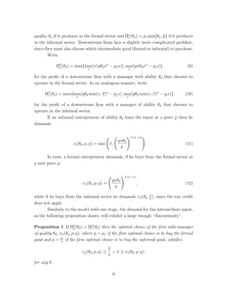
Each agent also has the choice of becoming a worker and receive the market
wage w. Hence the occupational choice cutoff points are implicitly defined by:
f () = i() (7)
max{i(ˆ),f (ˆ)} = w (8)
and optimal choices are:
ˆ =) Worker;
2 (ˆ, ] =) Informal entrepreneur;
max{, ˆ} =) Formal entrepreneur.
Since i(0) = 0 and f (0) = 0, ˆ 0, whenever w 0. However, if ˆ
then no entrepreneur would choose informality. In any case, equilibrium in the labor
market requires w to satisfy:
Z max{(w),ˆ(w)}
ˆ(w)
li(;w)g()d +
Z 1
max{(w),ˆ(w)}
lf (;w)g()d
| {z }
Demand for Labor
=
Z ˆ(w)
0
g()d
| {z }
Supply of Labor
where the arguments remind the reader of the dependence of the cutoffs and labor
demand on the level of wages.
The existence of an equilibrium level of wages is straightforward. Also if k
is large enough then ˆ. Furthermore if is sufficiently large, an entrepreneur of
quality would choose the formal sector.
Another implication of this model is the existence of a discontinuity in the level
of capital and labor employed at levels of productivity around . This discontinuity
7

32. follows since an entrepreneur with ability just below chooses the informal sector and
employs exactly k units of capital, although the marginal product of capital exceeds
his cost of capital. At a level just above , an entrepreneur chooses the formal sector
and since he is now unconstrained, he would choose a level k k. The jump in
the amount of capital employed also induces a jump in the marginal product of labor
and hence employment also exhibits a discontinuity at . Thus our model predicts a
“gap” in the quality distributions of firms.
3 A Model with Two Production Stages
In this section we introduce a model with two stages of production. Our goal is to
illustrate the transmission of informality across sectors which results from the use of
the value added tax. In Section 4 we document that this mechanism is relevant for
the generation of informality in Brazil.
There are two stages of production: “upstream” and “downstream”. All in-dividuals
in this model are entrepreneurs and, for simplicity, we assume that they
are specialized in one of the stages. Each entrepreneur in the upstream sector is
characterized by his ability u 0. The density of u is gu(·). An entrepreneur of
ability u can produce u units of the intermediate good in the formal sector, but
only min(y, u), where y 0, if in the informal sector.
The downstream entrepreneurs are characterized by an ability parameter d
with density gd(·). An agent with ability d, if in the formal sector, produces dx
units of the formal good using x units of the intermediate good. However if in the
informal sector he faces a limit on the quantity of input that can be used and the
production function becomes d min(x, x), where x 0.
We assume that gu and gd are continuous and positive on their support. In
addition we assume that there exists u y for which gu(u) 0, and that gd(d) 0
for d 0.
The final good is tradeable and has an exogenous price q. Firms in the formal
sector pay an ad-valorem tax rate of and we write = 1−. The value added tax is
levied by the credit method: the tax rate applies to each sale and each establishment
receives a credit for the amount of tax paid in the previous stages of production.
Because of the tax credit, the prices paid for informal and formal goods may be
distinct and we let pf be the price of the intermediate good in the formal sector and
pi in the informal sector.
We write uf
(u) = pf u for the profit of an upstream firm with manager of
8

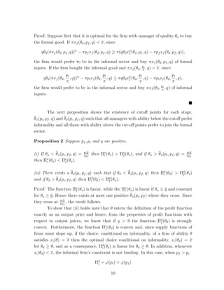
33. quality u if it produces in the formal sector and ui
(u) = pi min{u, y} if it produces
in the informal sector. Downstream firms face a slightly more complicated problem,
since they must also choose which intermediate good (formal or informal) to purchase.
Write
df
(d) = max{max
x
[(qdx − pfx)], max
x
[qdx − pix]}, (9)
for the profit of a downstream firm with a manager with ability d that chooses to
operate in the formal sector. In an analogous manner, write
di
(d) = max{max
x
[qd min(x, x) − pfx], max
x
[qd min(x, x) − pix]}, (10)
for the profit of a downstream firm with a manager of ability d that chooses to
operate in the informal sector.
If an informal entrepreneur of ability d buys the input at a price p then he
demands:
xi(d, p, q) = min
x,
qd
p
!1/(1−)!
. (11)
In turn, a formal entrepreneur demands, if he buys from the formal sector at
a unit price p:
xf (d, p, q) =
qd
p
!1/(1−)
, (12)
while if he buys from the informal sector he demands xf (d, p
), since the tax credit
does not apply.
Similarly to the model with one stage, the demand for the intermediate input,
as the following proposition shows, will exhibit a large enough “discontinuity”.
Proposition 1 If df
(d) di
(d) then the optimal choice of the firm with manager
of quality d, xf (d, p, q), where p = pf if the firm optimal choice is to buy the formal
good and p = pi
if the firm optimal choice is to buy the informal good, satisfies
xf (d, p, q)
x
x xi(d, p, q),
for any .
9

34. Proof: Suppose first that it is optimal for the firm with manager of quality d to buy
the formal good. If xf (d, pf , q) x, since
qd(xf (d, pf , q)) − pfxf (d, pf , q) (qdxf
(d, pf , q) − pfxf (d, pf , q)),
the firm would prefer to be in the informal sector and buy xf (d, pf , q) of formal
inputs. If the firm bought the informal good and xf (d, pi
, q) x, since
qd(xf (d,
pi
, q)) − pixf (d,
pi
, q) qdxf
(d,
pi
, q) − pixf (d,
pi
, q),
the firm would prefer to be in the informal sector and buy xf (d, pi
, q) of informal
inputs.
The next proposition shows the existence of cutoff points for each stage,
u(pi, pf , q) and d(pi, pf , q) such that all managers with ability below the cutoff prefer
informality and all those with ability above the cut-off points prefer to join the formal
sector.
Proposition 2 Suppose pf , pi and q are positive.
(i) If u u(pi, pf , q) = piy
pf
then ui
(u) uf
(u), and if u u(pi, pf , q) = piy
pf
then ui
(u) uf
(u).
(ii) There exists a d(pi, pf , q) such that if d d(pi, pf , q) then di
(d) df
(d)
and if d d(pi, pf , q) then di
(d) df(u).
Proof: The function uf
(u) is linear, while the ui
(u) is linear if u y and constant
for u y. Hence there exists at most one positive u(pi, pf ) where they cross. Since
they cross at piy
pf
, the result follows.
To show that (ii) holds note that enters the definition of the profit function
df
exactly as an output price and hence, from the properties of profit functions with
respect to output prices, we know that if q 0 the function (d) is strongly
convex. Furthermore, the function uf
(d) is convex and, since supply functions of
firms must slope up, if the choice, conditional on informality, of a firm of ability
satisfies xi() = x then the optimal choice conditional on informality, xi(d) = x
for d , and as a consequence, di
(d) is linear for d . In addition, whenever
xi(d) x, the informal firm’s constraint is not binding. In this case, when pf pi
di
= '(pi) '(pf )
10

35. where '(p) = [/(1−) − 1/(1−)]
qd
p
1/(1−)
. since
df
= max{'(pf ), 1/(1−)'(pi)}
then di
(d) df
(d). When pf pi,
di
= '(pf ) '(pi)
and the definition of df
(d) guarantees that di
(d) df
(d). In summary, whenever
xi(d) x, one obtains that di
(d) df
(d). Hence there is exactly one crossing
point, u(pi, pf , q).
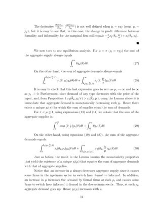
We now derive aggregate demand and supply of the intermediate good in the
formal and informal sectors as a function of prevailing prices. Since we are interested
in equilibrium prices we may restrict the range of prices to pf pi pf . In fact,
if pf pi profit maximization and equations (9) and (10) imply that both formal
and informal entrepreneurs downstream would buy from informal upstream firms.
However, every upstream entrepreneur will prefer to produce in the formal sector.
Similarly, if pi pf every downstream entrepreneur would prefer to buy from formal
firms. However, small u agents would prefer to produce informally. In addition,
the homogeneity of the system allows us to choose q = 1 (and hence we omit q as a
function argument in what follows).
Because of the possibility of indifference, we have supply and demand corre-spondences
as opposed to functions. We will write S(pi, pf ) for the set of possible
aggregate supply vectors (si(pi, pf ), sf (pi, pf )) obtained from the choices of profit max-imizing
entrepreneurs in the upstream stage. If pi6= pf the set S(pi, pf ) contains a
single vector (si, sf ) given by
si =
Z piy
pf
0
max{, y}gu()d (13)
sf =
Z 1
piy
pf
gu()d (14)
If pf = pi = 0 then S(pi, pf ) = {0}. Finally when pf = pi6= 0 a point (si, sf ) 2
11

36. S(pi, pf ) if there exists a u y such that:5
si =
Z u
0
gu()d (15)
sf =
Z 1
u
gu()d (16)
Since we fixed q = 1 we write X(pi, pf ) for the set of possible aggregate
demand vectors (xi(pi, pf ), xf (pi, pf )) obtained from the choices of profit maximizing
entrepreneurs in the downstream stage.
When pf = pi formal firms are indifferent between buying the formal or
informal input, but informal firms prefer buying from informal firms. Hence we
can allocate all formal firms with managers below a certain threshold to buying in
the informal sector with the complement interval assigned to purchase in the formal
sector.6 In this case, a point (xi, xf ) 2 X(pi, pf ) if there exists a
d(pi, pf , 1) such
that:
xi =
Z d(pi,pf ,1)
0
xi(d, pi)gd()d +
Z
d(pi,pf ,1)
xf (d,
pi
)gd()d (17)
xf =
Z 1
xf (d, pf )gd()d (18)
If pf pi pf formal (informal) firms prefer to buy from formal (informal)
firms. In this case, a point (xi, xf ) 2 X(pi, pf ) if :
xi =
Z d(pi,pf ,1)
0
xi(d, pi)gd()d (19)
xf =
Z 1
d(pi,pf ,1)
xf (d, pf )gd()d (20)
If pf = pi informal firms are indifferent, but formal firms prefer buying from
formal firms. Hence we may assign informal firms arbitrarily to buying formal or in-formal
inputs. In this case, a point (xi, xf ) 2 X(pi, pf ) if there exists
d(pi, pf , 1)
such that:
xi =
Z
0
xi(d, pi)gd()d (21)
xf =
Z d(pi,pi,1)
xi(d, pi)gd()d +
Z 1
d(pi,pi,1)
xf (d, pi)gd()d (22)
5In principle we could assign any subset of the entrepreneurs with productivity below y to the
informal sector, but there is always an interval containing the origin of these entrepreneurs that
would produce exactly the same aggregate output.
6As before, these assignments can reproduce the demands realized by any arbitrary assignment
of firms to each sector.
12

37. An equilibrium is a vector (pi, pf , 1) such that 9z 2 X(pi, pf )
T
S(pi, pf ).
We will decompose the proof of the existence of an equilibrium price in two
steps. First we will set pi = μpf with μ 1. For each μ we will show that there
exists a unique pi(μ) such that if (pi, pf ) = (pi(μ), pi(μ)
μ ) then the sum of aggregate
supply of the formal and informal intermediate goods equals the sum of aggregate
demands. We then show that there exits a unique μ such that (pi(μ), pi(μ)
μ , 1) is an
equilibrium.
We will use a preliminary result:
Lemma 1 If pf pi pf then d(pi, pf , 1) decreases with pi and it increases with
pf . Further, if μ 1 then, d(pi, pi
μ , 1) increases with pi.
Proof: If pf pi pf formal firms prefer to buy the formal good. Hence from
equations (9) and the envelope theorem,
@df
(d)
@pf
= −xf (d, pf ) (23)
Similarly, if pf pi pf , informal firms prefer to buy the informal good,
and in an analogous fashion, using equation (10)
@di
(d)
@pi
= −xi(d, pi) (24)
This establishes the first part of the lemma since increasing pi reduces profits
for informal firms and increasing pf reduces profits for formal firms.
In order to sign the change in d(pi, pi
μ , 1) we must establish the sign of:
1
μ
@df
(d)
@pf
−
@di
(d)
@pi
. (25)
for the marginal firm. If this is negative, the difference in profits in the formal and
informal sectors for the marginal firm decreases and more firms will become informal.
If pi pf pi, from equations (23) and (24)
1
μ
@df
(d)
@pf
−
@di
(d)
@pi
= −
μ
xf (d,
pi
μ
) + xi(d, pi). (26)
The marginal informal firm buys exactly x. Hence, from Proposition 1
−
μ
xf (d,
pi
μ
) + xi(d, pi) −
x
μ
+ x 0
since we assume that μ 1 and the second part of the lemma follows.
13

38. The derivative
@df
(d)
@pf
( @di
(d)
@pi
) is not well defined when pi = pf (resp. pi =
pf ), but it is easy to see that, in this case, the change in profit difference between
formality and informality for the marginal firm still equals −
μxf (d, pi
μ ) + xi(d, pi).
We now turn to our equilibrium analysis. For μ = (pi = pf ) the sum of
the aggregate supply always equals
Z 1
0
gu()d. (27)
On the other hand, the sum of aggregate demands always equals
Z d(pi, pi
,1)
0
xi(, pi)gd()d +
Z 1
d(pi, pi
,1)
xf (,
pi
)gd()d (28)
It is easy to check that this last expression goes to zero as pi ! 1 and to 1
as pi ! 0. Furthermore, since demand of any type decreases with the price of the
input, and, from Proposition 1 xf (d, pi/) xi(d, pi), using the Lemma above it is
immediate that aggregate demand is monotonically decreasing with pi. Hence there
exists a unique pi() for which the sum of supplies equal the sum of demands.
For μ 1, using expressions (13) and (14) we obtain that the sum of the
aggregate supplies is:
Z μy
0
max{, y}gu()d +
Z 1
μy
gu()d. (29)
On the other hand, using equations (19) and (20), the sum of the aggregate
demands equals:
Z d(pi, pi
μ ,1)
0
xi(d, pi)gd()d +
Z 1
d(pi,pi/μ,1)
xf (d,
pi
μ
)gd()d. (30)
Just as before, the result in the Lemma insures the monotonicity properties
that yield the existence of a unique pi(μ) that equates the sum of aggregate demands
with that of aggregate supplies.
Notice that an increase in μ always decreases aggregate supply since it causes
some firms in the upstream sector to switch from formal to informal. In addition,
an increase in μ increases the demand by formal firms at each pi and causes some
firms to switch from informal to formal in the downstream sector. Thus, at each pi,
aggregate demand goes up. Hence pi(μ) increases with μ.
14