Slide 1- 2
Readings
TEXTBOOK
[1] Ramez Elmasri and Shamkant B. Navathe,
Fundamentals of Database Systems, 5th Edition, 2007,
Addison-Wesley, ISBN 0-321-36957-2.
[2] Database System Concepts (Fourth Edition)
Abraham Silberschatz,Henry F. Korth,S. Sudarshan
3.
CONTENT
Introduction toData
Introduction to Database
Advantages of Data in Databse
Types of Databases and Database Applications
Database Implementation
Database Management System(DBMS)
Historical Development of Database Technology
Advantages of Database Management System
(DBMS)
Slide 1- 3
Slide 1- 5
Introductionto DATA
What is data?
Known facts that can be
recorded and have an
implicit meaning.
All the text, Graphics,
Images, Sound, Video
that have meaning in the
user environment.
A Data represent
information of the real
world.
Slide 1- 8
Introductionto Database
What is a database?
Collection of related data.
It is a collection of data that
are related in a meaningful
way, which can be accessed
in many different logical
order but are stored only
once.
It describing the activities of
one or more related
organizations.
e.g. Banking database,
University database.
Slide 1- 10
DatabaseDefinition
“A database has some source from which data are
derived, some degree of interaction with events in the real
world, and an audience that is actively interested in the
contents of the database”
Implicit Properties of a Database:
Represents some aspect of the real world (Mini-world).
A logically coherent collection of words with some inherent
meaning.
Designed, built & populated with data for a specific purpose.
Slide 1- 14
Typesof Databases and Database
Applications
Traditional Applications:
Numeric and Textual Databases
More Recent Applications:
Multimedia Databases
Geographic Information Systems (GIS)
Data Warehouses
Real-time and Active Databases
Many other applications
15.
Slide 1- 15
DatabaseImplementation
Defining a database
Data types
Structures
Constraints
Constructing a database
Storing the data itself on a storage medium
Manipulating a database
Querying
Updating
Generating reports
Slide 1- 17
DatabaseManagement System (DBMS)
General-purpose software system that facilitates the
processes of defining, constructing and manipulating
databases.
Can also write your own set of programs to create and
maintain the database, i.e. your own Special-purpose
DBMS software.
Database + Software == Database System
Slide 1- 23
HistoricalDevelopment of Database
Technology
Early Database Applications:
The Hierarchical and Network Models were introduced in
mid 1960s and dominated during the seventies.
A bulk of the worldwide database processing still occurs
using these models, particularly, the hierarchical model.
Relational Model based Systems:
Relational model was originally introduced in 1970, was
heavily researched and experimented within IBM Research
and several universities.
Relational DBMS Products emerged in the early 1980s.
24.
Slide 1- 24
HistoricalDevelopment of Database
Technology (continued)
Object-oriented and emerging applications:
Object-Oriented Database Management Systems
(OODBMSs) were introduced in late 1980s and early 1990s
to cater to the need of complex data processing in CAD and
other applications.
Their use has not taken off much.
Many relational DBMSs have incorporated object database
concepts, leading to a new category called object-relational
DBMSs (ORDBMSs)
Extended relational systems add further capabilities (e.g. for
multimedia data, XML, and other data types)
25.
Slide 1- 25
HistoricalDevelopment of Database
Technology (continued)
Data on the Web and E-commerce Applications:
Web contains data in HTML (Hypertext markup
language) with links among pages.
This has given rise to a new set of applications
and E-commerce is using new standards like XML
(eXtended Markup Language).
Script programming languages such as PHP and
JavaScript allow generation of dynamic Web
pages that are partially generated from a
database.
Also allow database updates through Web pages
Slide 1- 2
CONTENT
Summary of Basic Definitions of DBMS
Typical DBMS Functionality
Example of a Database (UNIVERSITY)
The Database Approach Vs File Processing
Approach
Advantages of Using the Database Approach
28.
Slide 1- 3
Summaryof Basic Definitions of
DBMS
Database:
A collection of related data.
Data:
Known facts that can be recorded and have an implicit meaning.
Mini-world:
Some part of the real world about which data is stored in a
database. For example, student grades and transcripts at a
university.
Database Management System (DBMS):
A software package/ system to facilitate the creation and
maintenance of a computerized database.
Database System:
The DBMS software together with the data itself. Sometimes, the
applications are also included.
Slide 1- 6
TypicalDBMS Functionality
Define a particular database in terms of its data types,
structures, and constraints
Construct or Load the initial database contents on a
secondary storage medium
Manipulating the database:
Retrieval: Querying, generating reports
Modification: Insertions, deletions and updates to its content
Accessing the database through Web applications
Processing and Sharing by a set of concurrent users and
application programs – yet, keeping all data valid and
consistent
32.
Slide 1- 7
TypicalDBMS Functionality
Other features:
Protection or Security measures to prevent
unauthorized access
“Active” processing to take internal actions on data
Presentation and Visualization of data
Maintaining the database and associated
programs over the lifetime of the database
application
Called database, software, and system
maintenance
33.
Slide 1- 8
Exampleof a Database
(with a Conceptual Data Model)
Mini-world for the example:
UNIVERSITY environment.
Some mini-world entities:
STUDENTs
COURSEs
SECTIONs (of COURSEs)
(academic) DEPARTMENTs
INSTRUCTORs
34.
Slide 1- 9
Exampleof a Database
(with a Conceptual Data Model)
Some mini-world relationships:
SECTIONs are of specific COURSEs
STUDENTs take SECTIONs
COURSEs have prerequisite COURSEs
INSTRUCTORs teach SECTIONs
COURSEs are offered by DEPARTMENTs
STUDENTs major in DEPARTMENTs
Note: The above entities and relationships are typically
expressed in a conceptual data model, such as the
ENTITY-RELATIONSHIP(E-R Model) data model.
35.
Slide 1- 10
Exampleof a simple database
Name Student_number Class Major
Smith 17 1 CS
Brown 8 2 CS
STUDENT
36.
Slide 1- 11
TheDatabase Approach Vs File
Processing Approach
In traditional file processing, each user defines and
implements the files needed for a specific application.
redundancy in defining and storing data.
wastes storage space and effort used to maintain the
common data up-to-date.
In the database approach, a single repository of data is
maintained that is defined once and then is accessed by
various users.
Slide 1- 16
Advantagesof Using the Database
Approach
Controlling redundancy in data storage and in
development and maintenance efforts.
Sharing of data among multiple users.
Restricting unauthorized access to data.
Providing persistent storage for program Objects
In Object-oriented DBMSs
Providing Storage Structures (e.g. indexes) for
efficient Query Processing
42.
Slide 1- 17
Advantagesof Using the Database
Approach (continued)
Providing backup and recovery services.
Providing multiple interfaces to different classes
of users.
Representing complex relationships among data.
Enforcing integrity constraints on the database.
Drawing inferences and actions from the stored
data using deductive and active rules
Slide 1- 2
CONTENT
Main Characteristics of the Database Approach
Additional Implications of Using the Database
Approach
When Not to Use Databases
Database Users
46.
Slide 1- 3
MainCharacteristics of the Database
Approach
Self-describing nature of a database system:
A DBMS catalog stores the description of a particular
database (e.g. data structures, types, and constraints)
The description is called meta-data.
This allows the DBMS software to work with different
database applications.
Insulation between programs and data:
Called program-data independence.
Allows changing data structures and storage organization
without having to change the DBMS access programs.
47.
Slide 1- 4
MainCharacteristics of the Database
Approach (continued)
Data Abstraction:
A data model is used to hide storage details and
present the users with a conceptual view of the
database.
Programs refer to the data model constructs rather
than data storage details
Support of multiple views of the data:
Each user may see a different view of the
database, which describes only the data of
interest to that user.
48.
Slide 1- 5
MainCharacteristics of the Database
Approach (continued)
Sharing of data and multi-user transaction
processing:
Allowing a set of concurrent users to retrieve from and to
update the database.
Concurrency control within the DBMS guarantees that each
transaction is correctly executed or aborted
Recovery subsystem ensures each completed transaction
has its effect permanently recorded in the database
OLTP (Online Transaction Processing) is a major part of
database applications. This allows hundreds of concurrent
transactions to execute per second.
49.
Slide 1- 6
AdditionalImplications of Using the
Database Approach
Potential for enforcing standards:
This is very crucial for the success of database
applications in large organizations. Standards
refer to data item names, display formats, screens,
report structures, meta-data (description of data),
Web page layouts, etc.
Reduced application development time:
Incremental time to add each new application is
reduced.
50.
Slide 1- 7
AdditionalImplications of Using the
Database Approach (continued)
Flexibility to change data structures:
Database structure may evolve as new
requirements are defined.
Availability of current information:
Extremely important for on-line transaction
systems such as airline, hotel, car reservations.
Economies of scale:
Wasteful overlap of resources and personnel can
be avoided by consolidating data and applications
across departments.
51.
Slide 1- 8
ExtendingDatabase Capabilities
New functionality is being added to DBMSs in the following areas:
Scientific Applications
XML (eXtensible Markup Language)
Image Storage and Management
Audio and Video Data Management
Data Warehousing and Data Mining
Spatial Data Management
Time Series and Historical Data Management
The above gives rise to new research and development in
incorporating new data types, complex data structures, new
operations and storage and indexing schemes in database systems.
52.
Slide 1- 9
Whennot to use a DBMS
Main inhibitors (costs) of using a DBMS:
High initial investment and possible need for additional
hardware.
Overhead for providing generality, security, concurrency
control, recovery, and integrity functions.
When a DBMS may be unnecessary:
If the database and applications are simple, well defined,
and not expected to change.
If there are stringent real-time requirements that may not be
met because of DBMS overhead.
If access to data by multiple users is not required.
53.
Slide 1- 10
Whennot to use a DBMS
When no DBMS may suffice:
If the database system is not able to handle the
complexity of data because of modeling limitations
If the database users need special operations not
supported by the DBMS.
54.
Slide 1- 11
DatabaseUsers
Users may be divided into
Actors on the Scene: Those who actually use
and control the database content, and those who
design, develop and maintain database
applications.
Workers Behind the Scene: Those who design
and develop the DBMS software and related tools,
and the computer systems operators.
55.
Slide 1- 12
DatabaseUsers
Actors on the scene
Database administrators:
Responsible for authorizing access to the database,
for coordinating and monitoring its use, acquiring
software and hardware resources, controlling its use
and monitoring efficiency of operations.
Database Designers:
Responsible to define the content, the structure, the
constraints, and functions or transactions against
the database. They must communicate with the
end-users and understand their needs.
Slide 1- 15
Slide 1- 17
Categoriesof End-users
Actors on the scene (continued)
End-users: They use the data for queries, reports
and some of them update the database content.
End-users can be categorized into:
Casual: access database occasionally when
needed.
Naïve or Parametric: they make up a large section
of the end-user population.
They use previously well-defined functions in the form of
“canned transactions” against the database.
Examples are bank-tellers or reservation clerks who do
this activity for an entire shift of operations.
61.
Slide 1- 18
Categoriesof End-users (continued)
Sophisticated:
These include business analysts, scientists, engineers,
others thoroughly familiar with the system capabilities.
Many use tools in the form of software packages that work
closely with the stored database.
Stand-alone:
Mostly maintain personal databases using ready-to-use
packaged applications.
An example is a tax program user that creates its own
internal database.
Another example is a user that maintains an address book
View of Data
A database system is a collection of interrelated files and a
set of programs that allow users to access and modify these
files.
A major purpose of a database system is to provide users
with an abstract view of the data.
Data Abstraction
For the system to be usable, it must retrieve data
efficiently. The need for efficiency has led designers to
use complex data structures to represent data in the
database.
Thus abstraction refers to hiding the complexity from
users through several levels of abstraction, to simplify
users’ interactions with the system.
65.
Data Abstraction
Data retrievalfrom database should be made easy
& efficient since database user are not computer
trained .
So the developer hide the complexity from user for
several level of abstraction.
Slide 1- 4
Physical level.(Physical schema describes the files and indexes used.)
The lowest level of abstraction describes how the data are actually
stored.
The physical level describes complex low-level data structures in detail.
The design of data structure is described at this level called physical
schema.
It specify that records are stored in either as pages.
Logical level. (Conceptual schema defines logical structure)
This is middle level of abstraction and it describes what data are
stored in the database, and what relationship exist among the
those data, there is only one schemas only for one database.
The logical level thus describes the entire database in terms of a small
number of relatively simple structures.
The logical level of abstraction is used by database administrator,
Who decide what information has to kept inside database.
View of Data
69.
View of Data
View level.(External schemata describe how users see the data. )
The highest level of abstraction describes only part of the entire
database. Even though the logical level uses simpler structures,
complexity remains because of the variety of information stored in
a large database.
Many users of the database system do not need all this
information; instead, they need to access only a part of the
database. The view level of abstraction exists to simplify their
interaction with the system. The system may provide many views
for the same database.
Slide 1- 8
Levels of Abstraction(Viewof Data)
Physical level: It describes how a record (e.g., customer)
is stored.
Logical level: describes data stored in database, and the
relationships among the data.
type customer = record
name : string;
street : string;
city : integer;
end;
View level: application programs hide details of data
types. Views can also hide information (e.g., salary) for
security purposes.
72.
Three-Schema Architecture
Thisidea was first described by the ANSI/SPARC
committee in late 1970's. The goal is to separate (i.e.,
insert layers of "insulation" between) user applications
and the physical database.
C.J. Date points out that it is an ideal that few, if any,
real-life DBMS's achieve fully.
Proposed to support DBMS characteristics of:
Program-data independence.
Support of multiple views of the data.
73.
Three-Schema Architecture
DefinesDBMS schemas at three levels:
Internal schema at the internal level to describe physical storage
structures and access paths (e.g indexes).
Typically uses a physical data model.
Conceptual schema at the conceptual level to describe the structure
and constraints for the whole database for a community of users.
Uses a conceptual or an implementation data model.
External schemas at the external level to describe the various user
views.
Usually uses the same data model as the conceptual schema.
Slide 1- 2
CONTENT
Three-Schema Architecture-Mapping
Data Independence
Logical Data Independence
Physical Data Independence
Difference between Logical and Physical Data
Independence
Data model Schema and Instance
Database Schema vs. Database State
81.
Three-Schema Architecture-Mapping
Mappingsamong schema levels are needed to
transform requests and data.
Programs refer to an external schema, and are
mapped by the DBMS to the internal schema for
execution.
Data extracted from the internal DBMS level is
reformatted to match the user’s external view.
(e.g. formatting the results of an SQL query for
display in a Web page)
82.
Data Independence
Applicationsinsulated from how data is structured and stored.
Data independence is the capacity to change the schema at
one level of the architecture without having to change the
schema at the next higher level.
We distinguish between logical and physical data independence
according to which two adjacent levels are involved.
Logical Data Independence:
The capacity to change the conceptual schema without having
to change the external schemas and their associated application
programs.
Physical Data Independence:
The capacity to change the internal schema without having to
change the conceptual schema.
For example, the internal schema may be changed when certain
file structures are reorganized or new indexes are created to
improve database performance.
83.
Logical Data Independence
Logical Data Independence- Ability to change the
conceptual schema without changing external schemas or application
programs.
Refers to immunity of external schemas to changes in conceptual
schema.
Conceptual schema changes (e.g. addition/removal of entities).
Should not require changes to external schema or rewrites of
application programs
Example: adding a field to a table should not affect other users view
of the data
84.
Physical Data Independence
Physical Data Independence- Ability to change the
internal (physical) schema without changing the conceptual schema.
Refers to immunity of conceptual schema to changes in the internal
schema.
Internal schema changes (e.g. using different file organizations, storage
structures/devices).
Should not require change to conceptual or external schemas.
Example: moving physical files from one disk to another. Easier to
implement than logical independence.
An example of physical data independence
suppose that the internal schema is modified (because we decide to
add a new index, or change the encoding scheme used in
representing some field's value, or stipulate that some previously
unordered file must be ordered by a particular field ). Then we can
change the mapping between the conceptual and internal schemas
in order to avoid changing the conceptual schema itself.
85.
Physical DataIndependence
Protection from changes in physical structure of data.
It is the ability to modify the physical schema without causing
application programs to be rewritten.
In other words, old programs do not have to be rewritten, when
changes are made to physical storage structure or the physical
devices on which data are stored.
Logical Data Independence:
Protection from changes in logical structure of data.
It is the ability to modify the conceptual schema without causing
application program to be rewritten.
Logical data independence is more difficult to achieve than physical
data independence, since program are having dependence the
logical structure of the database.
Difference between Logical and Physical Data
Independence
86.
Data model Schemaand Instance
The overall design of a database is called schema.
Similar to types and variables in programming languages
Schema – the logical structure of the database
e.g., the database consists of information about a set of customers
and accounts and the relationship between them
Analogous to type information of a variable in a program
Physical schema: database design at the physical level
Logical schema: database design at the logical level
A database may also have several schemas at the view level,
sometimes called subschemas, that describe different views of the
database.
87.
Database Schemas andTypes
Database Schema:
The description of a database.
Includes descriptions of the database structure,
data types, and the constraints on the database.
Schema Diagram:
An illustrative display of (most aspects of) a
database schema.
Schema Construct:
A component of the schema or an object within
the schema, e.g., STUDENT, COURSE.
88.
Database Schema
Adatabase schema is the skeleton structure of the
database. It represents the logical view of the entire
database.
A schema contains schema objects like table, foreign key,
primary key, views, columns, data types, stored procedure,
etc.
A database schema can be represented by using the visual
diagram. That diagram shows the database objects and
relationship with each other.
A database schema is designed by the database designers
to help programmers whose software will interact with the
database.
The process of database creation is called data modeling.
Slide 1- 10
89.
Database Schema
Aschema diagram can display only some aspects of a schema
like the name of record type, data type, and constraints. Other
aspects can't be specified through the schema diagram.
For example, the given figure neither show the data type of
each data item nor the relationship among various files.
In the database, actual data changes quite frequently.
For example, in the given figure, the database changes
whenever we add a new grade or add a student. The data at a
particular moment of time is called the instance of the
database.
Slide 1- 11
90.
Instances
Instance –the actual content of the database at a particular point
in time
Analogous to the value of a variable
Databases change over time as information is inserted and
deleted. The collection of information stored in the database at a
particular moment is called an instance of the database.
Example:
A program written in a programming language. A database
schema corresponds to the variable declarations (along with
associated type definitions) in a program. Each variable has a
particular value at a given instant. The values of the variables in
a program at a point in time correspond to an instance of a
database schema.
91.
Database State:
DatabaseState:
The actual data stored in a database at a
particular moment in time. This includes the
collection of all the data in the database.
Also called database instance (or occurrence or
snapshot).
The term instance is also applied to individual
database components, e.g. record instance, table
instance, entity instance
92.
Database Schema vs.Database State
Database State:
Refers to the content of a database at a moment in time.
Initial Database State:
Refers to the database state when it is initially loaded into the
system.
Valid State:
A state that satisfies the structure and constraints of the database.
Distinction
The database schema changes very infrequently.
The database state changes every time the database is updated.
Schema is also called intension.
State is also called extension.
Database Architecture
The architectureof a database systems is greatly
influenced by the underlying computer system on
which the database is running:
Centralized
Client-server
Parallel (multi-processor)
Distributed
Database System Structure
DBMS system are complicated or complex or may be some times
sophisticated. A DBMS has several software components Called
MODULES.
Each of which is assigned a specific function(components)–
QUERY PROCESSOR: A query processor is one of the major
components of a relational database or an electronic database in which
data is stored in tables of rows and columns. It complements the storage
engine, which writes and reads data to and from storage media.
It transforms queries into a series of low-level instruction directed to
database manager. It parses, analyses and converts a query by creating
database access code.
The Query Processor is a Structured Query Language (SQL) parser,
optimizer, and query execution engine. The Query Processor accepts and
executes SQL commands according to a chosen plan and interacts with
the Enterprise Database Server storage engine to return the expected
results. Slide 1- 6
101.
Component of DBMS
FILE MANAGER: A file manager is a software program that helps a user
manage all the files on their computer. For example, file managers allows
the user to view, edit, copy, and delete the files on their computer storage
devices. It manages the allocation of storage space on disk.
It maintains the list of structure or indexes if hashed files are used then
hashing function is used to generate record addresses. Then it passes
control to access method which either allow the data to be read or write
data to the buffer.
DML PRE-PROCESSOR: Data Manipulation Language pre-processor is
a component of DBMS that converts embedded DML commands to the
application program in the form of the functions that are called in the host
language.
It converts data manipulation language statements into standard function
call.
It must interact with the query processor to generate the appropriate code.
Slide 1- 7
102.
Component of DBMS
DDL-COMPILER: Data Description Language compiler processes
schema definitions specified in the DDL. It includes metadata information
such as the name of the files, data items and storage details of each file.
It converts data definition language statements into a set of tables
containing Meta data.
Data dictionary contains name and size of file, data type, storage details,
mapping information among schemas and constraints.
DATA DICTIONARY MANAGER: It is also known as System Catalogue.
It is accessed by most of the DBMS components. It is so important part of
the DBMS. It accesses, manages and maintains the data dictionary.
Data Dictionary, which stores metadata about the database. in particular
the schema of the database , names of the tables, names of attributes of
each table, length of attributes, and number of rows in each table.
Slide 1- 8
103.
Component of DBMS
Detailed information on physical database design such as storage
structure, access paths, files and record sizes.
Usage statistics such as frequency of query and transactions.
Data dictionary is used to actually control the data integrity, database
operation and accuracy.
DATABASE MANAGER: It controls data dictionary and access of the
database.
It is an interface between users and queries. Database manager accepts
queries and examines the external and conceptual schemas to
determine for conceptual records are required to satisfy the generated
request. Database manager then places a call to the file manager to
perform the request.
Some components of database manager are as follows-
AUTHORIZATION CONTROL: It checks for user have sufficient
authorization to access the system.
Slide 1- 9
104.
Component of DBMS
COMMAND PROCESSOR: After checking authority then it is to carry
out the operation then control is passed to command processor.
QUERY OPTIMIZER: It determines optimal strategy for query execution.
TRANSACTION MANAGER: It performs the required processing of
operations then it coordinates the transaction of the system.
SCHEDULER: It schedules concurrent operation or transaction of the
system.
RECOVERY MANAGER: Database in consistent state so that database
can be restored. Recovery Manager (RMAN) is an Oracle utility that can
back up, restore, and recover database files. The product is a feature of
the Oracle database server and does not require separate installation.
Recovery Manager is a client/server application that uses database
server sessions to perform backup and recovery.
Slide 1- 10
105.
BUFFER MANAGER:
Data between main and secondary memory for
transferring of the data.
It is also called Cache Manager.
The buffer manager is a software module of DBMS whose
responsibility is to serve to all the data requests and take
decision about choosing a buffer and to manage page
replacement. The buffer manager must ensure that the
number of buffers fits in the main memory.
Slide 1- 11
Component of DBMS
Centralized DBMS Architectures
Centralized DBMS:
Combines everything into single system including-
DBMS software, hardware, application programs,
and user interface processing software.
User can still connect through a remote terminal –
however, all processing is done at centralized site.
Client-server architecture
Thisis a network architecture in which each computer or host is on a
network can be either a client or a server.
It has two logical components:-
Servers are powerful computers or processes dedicated to managing
disk drives (file servers), printers (print servers), or network traffic
(network servers).
Clients are PCs or workstations on which users run applications. .
Clients rely on servers for resources, such as files, devices, and even
processing power.
Client and server computers are connected into a software.
Generally client responds for DBMS’s services.
DBMS processes these requests and return the result to client.
Client Server architecture generally uses GUI.
Slide 1- 4
113.
5
Client/Server systems
Operatein a networked environment Processing of an application
distributed between front-end clients and back-end servers.
Generally the client process requires some resource, which the
server provides to the client.
Clients and servers can reside in the same computer, or they can
be on different computers that are networked together, usually:
Client – Workstation (usually a PC) that requests and uses a service.
Server – Computer (PC/mini/mainframe) that provides a service.
For DBMS, server is a database server
114.
Components And Functions
It has three general components.
1. Client Application:-
“Client/server systems operate in a networked environment, splitting the
processing of an application between a front-end client and a back-end
processor.”
A client here stands an end user here it uses an application/ device it
may be computer - mobile etc. with software or application.
It issues a SQL statements for data access as central environment
which may be tools or user written applications.
Each time a client application executes it contacts a server to send a
request and awaits for a response when the response arrives the client
continues his processing.
Clients are easily build and require no special system privileges to
operate.
Slide 1- 6
115.
7
Client Application
Theclient is usually a browser such as Internet Explorer, Netscape
Navigator or Mozilla. Browsers interact with the server using a set of
instructions called protocols.
These protocols help in the accurate transfer of data through requests
from a browser and responses from the server.
client and server may reside on same computer both are intelligent and
Programmable.
There are many protocols available on the Internet. The World Wide
Web, which is a part of the Internet, brings all these protocols under one
roof.
You can, thus, use HTTP, FTP, Telnet, email etc. from one platform -
your web browser
116.
8
Applications that runon computers
Rely on servers for
Files
Devices
Processing power
Example: E-mail client
An application that enables you to send and receive e-mail
Client Application
Clients are Applications
117.
2. NetworkInterface:-
It enables client application to connect to the server and
can send SQL statements and receive results or error
message etc.
This layer transfer data between client to database server.
This layer uses web server / application to check request
from client.
It somewhere also converts the view of data according to
client requirement.
Slide 1- 9
Components And Functions
118.
3. DatabaseServer:-
A server is any program that provides services to requested process
from client / client applications.
This layer has all the data or we can say it is our main device or server
which has all information.
It take input / request from client application layer then process the
request and generate the response and forward it to the application
server.
Server Contains:-
1. Authentication:-Verifying identity of client.
2. Authorization:-Permission of Accessing Services.
3. Data Security:-Data is not compromised.
4. Privacy:-Information secured from unauthorized access.
5. Protection:- Network Application can not get unauthorized access of
system Resources.
Slide 1- 10
Components And Functions
119.
11
Database Server
Computers orprocesses that manage network resources
Disk drives (file servers)
Printers (print servers)
Network traffic (network servers)
Example: Database Server
A computer system that processes database queries
Servers Manage
Resources
120.
12
Types of Servers
Chat Servers
Fax Servers
FTP Servers
Groupware Servers
Mail Servers
121.
Application Architectures
Two-tier architecture:E.g. client programs using ODBC/JDBC to
communicate with a database
Three-tier architecture: E.g. web-based applications, and applications
built using “middleware”
16
Distributed Database Systemshave now come
to be known as client server based database
systems because they do not support a totally
distributed environment, but rather a set of
database servers supporting a set of clients.
Two-Tier Client-Server Architectures- Network
125.
17
Two-Tier Client-Server Architectures-Web View
User HTTP Request
Response to HTTP Request
Web Server
Client
Processing of HTML code takes place on the client side
and the web page request is processed on the server side
Two-Tier Client-Server Architectures
Specialized Servers with Specialized functions
Print server
File server
DBMS server
Web server
Email server
Clients can access the specialized servers as
needed.
128.
Clients
Provide appropriateinterfaces through a client
software module to access and utilize the various
server resources.
Clients may be diskless machines or PCs or
Workstations with disks with only the client
software installed.
Connected to the servers via some form of a
network.
LAN: local area network, wireless network, etc.
129.
DBMS Server
Providesdatabase query and transaction services to the
clients
Relational DBMS servers are often called SQL servers,
query servers, or transaction servers
Applications running on clients utilize an Application
Program Interface (API) to access server databases via
standard interface such as:
ODBC: Open Database Connectivity standard
JDBC: for Java programming access
Client and server must install appropriate client module and
server module software for ODBC or JDBC
24
1. User HTTPRequest
4. Response to HTTP Request
Web Server
Client
DBMS
2
3
In a 3-tier architecture, we can place our database
management system or application software on a
different processing zone or tier than the web server
Three-tier client-server architecture
Three-Tier Client-Server Architecture
Common for Web applications
Intermediate Layer called Application Server or Web
Server:
Stores the web connectivity software and the business
logic part of the application used to access the
corresponding data from the database server
Acts like a conduit for sending partially processed data
between the database server and the client.
Three-tier Architecture Can Enhance Security:
Database server only accessible via middle tier
Clients cannot directly access database server
135.
27
• Application serverin addition to client and database server
• Thin clients: do less processing
• Application server contains “standard” programs
Benefits:
scalability
technological flexibility
lower long-term costs
better match business needs
improved customer service
competitive advantage
reduced risk
Three-Tier Client-Server Architecture
Slide 1- 2
CONTENT
Main Characteristics of Database Approach
Data Model
Classification of Data Model
History of Data Model
Hierarchical Data Model
Network Data Model
Relational Data Model
138.
C Self‐describing natureof a database system: A DBMS catalog
stores the description of the database. The description is called
meta‐data). This allows the DBMS software to work with
different databases.
C Insulation between programs and data: Called program‐data
independence. Allows changing data storage structures and
operations without having to change the DBMS access
programs.
C Data Abstraction: A data model is used to hide storage details
and present the users with a conceptual view of the database.
139.
C Support ofmultiple views of the data: Each user may see
a different view of the database, which describes only
the data of interest to that user.
C Sharing of data and multiuser transaction processing :
allowing a set of concurrent users to retrieve and to
update the database. Concurrency control within the
DBMS guarantees that each transaction is correctly
executed or completely aborted. OLTP (Online
Transaction Processing) is a major part of database
applications.
140.
A databasemodel referred as data model that determines the logical
structure of a database and fundamentally determines in which
manner data can be stored, organized and manipulated.
The most popular example of a database model is the relational model,
which uses a table-based format.
THE IMPORTANCE OF DATA MODELS--
Data model
Relatively simple representation, usually graphical, of complex real-
world data structures
Communications tool to facilitate interaction among the designer, the
applications programmer, and the end user
Good database design uses an appropriate data model as its foundation
Data model organizes data for various users.
Slide 1- 5
Data Model
141.
6
Data Models
DataModel: A set of concepts to describe the structure of
a database, and certain constraints that the database
should obey.
Data Model Operations: Operations for specifying
database retrievals and updates by referring to the
concepts of the data model. Operations on the data model
may include basic operations and user-defined
operations.
A collection of tools for describing
Data
Data relationships
Data semantics
Data constraints
142.
7
Categories of datamodels
Conceptual (high-level, semantic) data models:
Provide concepts that are close to the way many users
perceive data. (Also called entity-based or object-based
data models.)
Physical (low-level, internal) data models:
Provide concepts that describe details of how data is
stored in the computer.
Implementation (representational) data models:
Provide concepts that fall between the above two,
balancing user views with some computer storage details.
143.
Classification of DataModels-
• Based on the data model used:
• Traditional:
-Relational,
-Network,
-Hierarchical.
• Emerging: Object-based data models
-Object-oriented,
-Object-relational.
Entity-Relationship data model (mainly for database design)
Semi-structured data model (XML)
Slide 1- 8
It isintegrated collection of concept for manipulating data
and relationship between data. It has some basic models:-
1) FILE BASED SYSTEM or PRIMITIVE MODEL-
The entities or object are represented by records that are stored
together in files. Relationship between objects are represented by
directory.
2) TRADITIONAL DATA MODEL-
They are based on records.
For example - Hierarchical data model, Network data model and
Relational data model.
3) SEMANTIC DATA MODEL-
It is come from semantic network developed by artificial intelligence.
Semantic network is used for organizing and representing general
knowledge.
Slide 1- 10
Classification of Data Models-
146.
History of DataModels
Hierarchical Data Model: implemented in a joint effort by IBM
and North American Rockwell around 1965.
Resulted in the IMS family of systems. The most popular model.
Other system based on this model: System 2k (SAS inc.)
Relational Model: proposed in 1970 by E.F. Codd (IBM), first
commercial system in 1981-82. Now in several commercial
products (DB2, ORACLE, SQL Server, SYBASE, INFORMIX).
Network Model: the first one to be implemented by Honeywell in
1964-65 (IDS System). Adopted heavily due to the support by
CODASYL (CODASYL - DBTG report of 1971).
Later implemented in a large variety of systems - IDMS (Cullinet -
now CA), DMS 1100 (Unisys), IMAGE (H.P.), VAX -DBMS (Digital
Equipment Corp.).
147.
12
History of DataModels
Object-oriented Data Model(s): O-O Programming
Languages such as C++ (e.g., in OBJECTSTORE or
VERSANT), and
Smalltalk (e.g., in GEMSTONE).
Additionally, systems like O2, ORION (at MCC - then
ITASCA), IRIS (at H.P.- used in Open OODB).
Object-Relational Models:
Most Recent Trend. Started with Informix Universal Server.
Exemplified in the latest versions of Oracle-10i, DB2, and
SQL Server etc. systems.
So, several models have been proposed for implementing in
a database system.
148.
It isthe oldest form of data base model.
It was developed by IBM for IMS (information Management System).
It is a set of organized data in tree structure. DB record is a tree
consisting of many groups called segments.
It uses one to many relationships.
The data access is also predictable.
APPLICTIONS:-
1)It is a semantic model because of real world phenomenon.
e.g.-social structure or biological structure etc.
2)Physical model-you can see it is in the form of disc storage.
ADVANTAGES:-
1)Simplicity- due to simple design of tree structure .
2)Data sharing- due to centralization.
Slide 1- 13
Hierarchical Data Model
149.
3) Data security-because of database management system.
4) Efficiency- because of support of large data which may have one
to many relationships.
DISADVANTAGES:-
1) Implementation complexity- because of physical storage.
2) Inflexibility- because of changes in one segment can affect
another segment.
3) Changes in DBMS causes of changes in application program.
4) It has no standard.
5) Implementation limitation due to many to many relationship that
supports of real life problem.
6) Navigational and procedural nature of processing.
7) Database is visualized as a linear arrangement of records.
8) Little scope for "query optimization" Slide 1- 14
Hierarchical Data Model
150.
-It isan alternative to hierarchical data model.
-Formalized by DBTG(Data Base Task Group).
-It provides multiple path among segments.
-This model allows having one to one, one to many and many to many
relationship.
-Data modeling in it has a set construct. A set consist a set name, an
owner record type and member record type. A member record type can
have role in more than one set. It introduces the concept of multi-parent
concept.
- A network database stores information in data sets which are similar to
files and tables.
-Multiple paths eliminates some of the drawbacks of hierarchical
database model but it causes a new disadvantage. i.e. maintaining all
the links or you can say that relationship between them.
-Relationship are hierarchical in manner i.e., pre computed.
Slide 1- 15
Network Data Model
151.
The networkmodel is a database model conceived as a flexible way of
representing objects and their relationships.
Its distinguishing feature is that the schema, viewed as a graph in which
object types are nodes and relationship types are arcs, is not restricted
to being a hierarchy or lattice.
Slide 1- 16
Network Data Model
ADVANTAGES:-
1)Simplicity dueto easy design.
2) More relationship i.e., one to one, one to many or many to many which
helps in modeling real life.
3)Data access is here because of owner record type can access all member
record type.
4) Data integrity- A member does not exist without of owner. A user must
define both.
5)Standard DBTG.
6) Network Model is able to model complex relationships and represents
semantics of add/delete on the relationships.
7) Can handle most situations for modeling using record types and
relationship types.
8) Language is navigational; uses constructs like FIND, FIND member, FIND
owner, FIND NEXT within set, GET etc. Programmers can do optimal
navigation through the database. Slide 1- 18
Network Data Model
154.
19
Network Data Model
DISADVANTAGES:-
System complexity- The records maintained using pointers
so whole database structure gets more complex.
Not user friendly- It is designed by highly skilled
professionals.
The structural changes to the database is very difficult.
Navigational and procedural nature of processing.
Database contains a complex array of pointers that thread
through a set of records.
Little scope for automated "query optimization”
NOTION OF RELATION
Atable is said to be a relation, if it satisfies
following properties: -
• It is column homogeneous.
All items in a column are of the same kind.
• Each column is atomic.
Each item is an integer or a character string.
161.
• All rowsare distinct.
No two rows may be identical in every column.
• The ordering of rows is immaterial(Not Important).
• The ordering of columns is immaterial and they are assigned
distinct names.
NOTE: the first and third properties holds normally for any table. The
rest are specific to the relational model.
NOTION OF RELATION
162.
S# P# Sc
101 Delhi
10 2 Delhi
11 1 Mumbai
11 2 Mumbai
S# P# City
11 1 Delhi
11 1 Delhi
Name Child
Johnny,12-04-1985
Robert
Invalid relation
Child field is not atomic.
Invalid relation
Two rows are not
distinct.
A valid relation
163.
Identify whether thegiven relation is valid or invalid. Justify
reasons in support.
Customer – name Security-number Address City
Williams 321-12-3123 Downhill Banglore
Rama 321-12-3122 Downhill Banglore,
Hyderabad
Jaya 321-14-4562 Model Town Delhi
Jones 321-12-3123R
MG Road
Madras
Smith 321-14-9012 Main town Calcutta
Jaya 321-14-4562 Model Town Delhi
164.
• Domain isthe set of values over which the relation is constructed
integer and character strings
•Given n-domains ( D1 , D2 , ….., Dn ) , relation R is constructed as
R(D1, D2,…., Dn) X (D1, D2,……, Dn)
• Degree of relation R is n or it is a n-ary since it is defined over n
domains ( D1 , D2 , ….., Dn )
A Relation
• A ternary relation :
Mumbai
2
11
Mumbai
1
11
Delhi
3
10
Delhi
2
10
Delhi
1
10
Sc
P#
S#
165.
Relation Definition andRelation
• Definition of relation gives a name to the relation and specifies the
attributes over which it is built.
Relation Definition
Customer(Customer-name, Date-of-birth, Address)
• Relation is a set of tuples which constitutes it at a given instant of time
Goa
22-02-78
Harry
Delhi
12-04-78
john
Address
Date-of-Birth
Customer-
name
Relation may change with time while its definition remains same.
166.
Relational Schema
A relationalschema is a collection of relation definitions
Schema
RD1 , RD2,……………………RDn
Relational Schema does not change over time.
167.
Relational Model Concepts
The relational Model of Data is based on the concept of a
Relation.
A Relation is a mathematical concept based on the ideas of
sets.
The strength of the relational approach to data management
comes from the formal foundation provided by the theory of
relations.
168.
Relational Model Concepts
The model was first proposed by Dr. E.F. Codd of
IBM in 1970 in the following paper:
"A Relational Model for Large Shared Data Banks,"
Communications of the ACM, June 1970.
The above paper caused a major revolution in the field of
Database management and earned Ted Codd the coveted
ACM Turing Award.
169.
INFORMAL DEFINITIONS
RELATION:A table of values
A relation may be thought of as a set of rows.
A relation may alternately be though of as a set of
columns.
Each row represents a fact that corresponds to a real-
world entity or relationship.
Each row has a value of an item or set of items that
uniquely identifies that row in the table.
Sometimes row-ids or sequential numbers are assigned to
identify the rows in the table.
Each column typically is called by its column name or
column header or attribute name.
170.
FORMAL DEFINITIONS
ARelation may be defined in multiple ways.
The Schema of a Relation: R (A1, A2, .....An)
Relation schema R is defined over attributes A1, A2, .....An
For Example -
CUSTOMER (Cust-id, Cust-name, Address, Phone#)
Here, CUSTOMER is a relation defined over the four
attributes Cust-id, Cust-name, Address, Phone#,
each of which has a domain or a set of valid values.
For example, the domain of Cust-id is 6 digit numbers.
171.
FORMAL DEFINITIONS
Tuple-
Atuple is an ordered set of values
Each value is derived from an appropriate domain.
Each row in the CUSTOMER table may be referred to as a
tuple in the table and would consist of four values.
<632895, "John Smith", "101 Main St. Atlanta, GA 30332", "(404) 894-2000">
is a tuple belonging to the CUSTOMER relation.
A relation may be regarded as a set of tuples (rows).
Columns in a table are also called attributes of the relation.
172.
FORMAL DEFINITIONS
Domain-
Adomain has a logical definition:
e.g., “USA_phone_numbers” are the set of 10 digit phone
numbers valid in the U.S.
A domain may have a data-type or a format defined for it.
The USA_phone_numbers may have a format: (ddd)-ddd-
dddd where each d is a decimal digit.
E.g., Dates have various formats such as monthname, date,
year or yyyy-mm-dd, or dd mm,yyyy etc.
An attribute designates the role played by the domain.
E.g., the domain Date may be used to define attributes
“Invoice-date” and “Payment-date”.
173.
Domains and Attributes
Domain- The set of values on which an attribute is defined
• Domain is concerned with data of type integer or character
strings
• Attribute is the meaning behind the domain
D1
D2
Customer-name Address Date-of-birth
Attribute
Character
string
Integer
FORMAL DEFINITIONS
Therelation is formed over the Cartesian product of the
sets; each set has values from a domain; that domain is
used in a specific role which is conveyed by the attribute
name.
For example, attribute Cust-name is defined over the
domain of strings of 25 characters. The role these strings
play in the CUSTOMER relation is that of the name of
customers.
Formally, Given R(A1, A2, .........., An)
r(R) dom (A1) X dom (A2) X ....X dom(An)
R: schema of the relation
r of R: a specific "value" or population of R.
R is also called the intension of a relation
r is also called the extension of a relation
176.
FORMAL DEFINITIONS
LetS1 = {0,1}
Let S2 = {a,b,c}
Let R S1 X S2
Then for example:
r(R) = {<0,a> , <0,b> , <1,c> }
is one possible “state”,
or “population”,
or “extension” r of the relation R,
defined over domains S1 and S2.
It has three tuples.
177.
DEFINITION SUMMARY
Informal TermsFormal Terms
Table Relation
Column Attribute/Domain
Row Tuple
Values in a column Domain
Table Definition Schema of a
Relation
Populated Table Extension
178.
Relational Model Constraints
The state of whole database will correspond to
state of all its relation at a particular point in time.
There are many constraints on actual values in a
database state.
They are:-
Inherent Model Constraint
Explicit Or Schema based constraint
Application based constraint
179.
Integrity Constraints
Ensures dataconsistency during modification of database
• Domain: a homogeneous set of values
• Key
• Entity Integrity
• Referential Integrity
On single relations only
Across relations
180.
Object-Relational Data Models
Relational model: flat, “atomic” values
Object Relational Data Models
Extend the relational data model by including object
orientation and constructs to deal with added data types.
Allow attributes of tuples to have complex types,
including non-atomic values such as nested relations.
Preserve relational foundations, in particular the
declarative access to data, while extending modeling
power.
Provide upward compatibility with existing relational
languages.
181.
Database Design
LogicalDesign – Deciding on the database schema.
Database design requires that we find a “good” collection of
relation schemas.
Business decision – What attributes should we record in
the database?
Computer Science decision – What relation schemas
should we have and how should the attributes be
distributed among the various relation schemas?
Physical Design – Deciding on the physical layout of the
database
The process of designing the general structure of the
database:
Design Approaches
Needto come up with a methodology to ensure that each of
the relations in the database is “good”
Two ways of doing so:
Entity Relationship Model
Models an enterprise as a collection of entities and
relationships
Represented diagrammatically by an entity-relationship
diagram:
Normalization Theory
Formalize what designs are bad, and test for them
DBMS Languages
1. DataDefinition Language (DDL): used (by the DBA
and/or database designers) to specify the conceptual
schema.
2. Data Manipulation Language (DML): used for performing
operations such as retrieval and update upon the
populated database.
3. Storage Definition Language (SDL): It is used to specify
the internal or physical schema.
In it, the storage structure and access methods used by the
DB system, is specified by a set of statements.
These statements define the implementation details of the
database schema.
188.
• High Levelor Non‐procedural Languages:
• e.g., SQL, are set‐oriented and specify what data to retrieve
than how to retrieve. Also called declarative languages.
• Low Level or Procedural Languages:
• they specify how to retrieve data and include constructs such
as looping.
DBMS Languages
189.
It isa set of SQL commands used to create, modify & delete
database structure but not data. These commands are used by
DBA.
DDL also updates data dictionary or data directory. A data
dictionary contains metadata i.e. data about data. The schema of a
table is an example of metadata.
A database system consults the data dictionary before reading or
modifying actual data.
The DBMS will have DDL compiler whose function is to process
DDL statement in order to identify description of the schema
constructs and to store the schema description in the DBMS
catalogue.
A language is needed to describe the database to the DBMS as
well as provide facilities for changing the database and for defining
and changing physical data structure. Slide 1- 6
1. Data Definition Language (DDL)
190.
DDL specifies howthe data is related.
E.g. schema
In terms of architecture the DDL involves following component:-
1. System catalogue:- Schema is stored here.
2. DDL compiler:- It translate the DDL into action.
3. Privileged commands:- An Action that only DBA can do.
Functionality of DDL:-
1. Creation of data structure supported by data model.
Eg. Create table for the relational model.
2. Modification of data structure. Eg. ALTER TABLE
3. Deletion of data structure. eg. DROP TABLE
4. Creating index. E.g. CREATE INDEX
Slide 1- 7
1. Data Definition Language (DDL)
191.
◗ In manyDBMSs, the DDL is also used to define internal and
external schemas (views).
◗ In some DBMSs, separate storage definition language (SDL) and
view definition language (VDL) are used to define internal and
external schemas.
1. Data Definition Language (DDL)
192.
Specification notationfor defining the database schema
Example: create table instructor (
ID char(5),
name varchar(20),
dept_name varchar(20),
salary numeric(8,2));
DDL compiler generates a set of table templates stored in a data dictionary
Data dictionary contains metadata (i.e., data about data)
Database schema
Integrity constraints
Primary key (ID uniquely identifies instructors)
Authorization
Who can access what
Data storage and definition language
language in which the storage structure and access methods used by
the database system are specified
Usually an extension of the data definition language
1. Data Definition Language (DDL)
193.
2. Data ManipulationLanguage
Data manipulation involves retrieval of data from the database,
Insertion of new data and Deletion on modification of existing data.
Data manipulation operation is called a query.
A query is a statement in the DML that requests the retrieval of data
from the database.
The subset of the DML used to pose a query is knows as query
language.
DML and query language approximately synonyms.
There are basically two types of DML
1. Procedural:- which requires a user to specify what data is needed
and how to get the algorithm is written in query language. eg. SQL,
Quel.
2. Non-Procedural:- specify what data is needed without specifying
how to get it. E.g. Datalog, QBE.
Slide 1- 10
194.
Functionality:-
1. Retrieval ofdata.
eg. Select operator for the relational model.
2. Modification of data.
eg. Update operator
3. Creation OR Insertion of data.
eg. INSERT operator
4. Deletion of data.
eg. Deletion operator
5. Most DML's have built in fn.
e.g. SUM, COUNT, AVG etc.
Slide 1- 11
2. Data Manipulation Language
195.
Language foraccessing and manipulating the data organized by the appropriate
data model
DML also known as query language
Two classes of languages
Procedural – user specifies what data is required and how to get those data
Nonprocedural – user specifies what data is required without specifying how
to get those data
Two classes of languages
Pure – used for proving properties about computational power and for
optimization
Relational Algebra
Tuple relational calculus
Domain relational calculus
Commercial – used in commercial systems
SQL is the most widely used commercial language
2. Data Manipulation Language
196.
• Used tospecify database retrievals and updates.
• DML commands (data sublanguage) can be embedded
in a general‐purpose programming language (host language),
such as COBOL, C or an Assembly Language.
• Alternatively, stand‐alone DML commands can be applied
directly (query language).
2. Data Manipulation Language
197.
DBMS Interfaces
1. Stand-alonequery language interfaces
Example: Entering SQL queries at the DBMS
interactive SQL interface.
(e.g. SQL*Plus in ORACLE)
198.
2. DBMS ProgrammingLanguage Interfaces
Programmer interfaces for embedding DML in programming
languages:
Embedded Approach: e.g embedded SQL (for C, C++,
etc.), SQLJ (for Java).
Procedure (Subroutine) Call Approach:
e.g. JDBC for Java, ODBC for other programming
languages.
Database Programming Language Approach: e.g.
ORACLE has PL/SQL, a programming language based
on SQL; language incorporates SQL and its data types
as integral components.
199.
3. User-Friendly DBMSInterfaces
Menu-based, popular for browsing on the web
Forms-based, designed for naïve users
Graphics-based
(Point and Click, Drag and Drop, etc.)
Natural language: requests in written English
Combinations of the above:
For example, both menus and forms used
extensively in Web database interfaces
200.
Other DBMS Interfaces
Speech as Input and Output
Web Browser as an interface
Parametric interfaces, e.g., bank tellers using
function keys.
Interfaces for the DBA:
Creating user accounts, granting authorizations
Setting system parameters
Changing schemas or access paths
Entity-Relationship Model
Content:
DataModeling Using Entity-Relationship Approach
Data Modeling In the Context of Database Design
Entity-Relationship Model(e-r model)
E-R Model Concepts
Attribute
Types of Attributes
Entity/entities
Entity Sets
Entity types
A relationship
203.
Data Modeling UsingEntity-Relationship
Approach
Introduction
A Data model is a conceptual representation of the data
structures that are required by a database.
The data structures include the data objects, the
associations between data objects, and the rules which
govern operations on the objects.
A Data model focuses on what data is required and how it
should be organized rather than what operations will be
performed on the data.
A Data model is equivalent to an architect's building plans.
A Data model is independent of hardware or software
constraints.
204.
The data modelfocuses on representing the data as the user
sees it in the "real world". It serves as a bridge between
the concepts that make up real-world events and
processes and the physical representation of those
concepts in a database.
Methodology
There are two major methodologies used to create a data
model:
1. Entity-Relationship (ER) approach and
2. Object Model.
Data Modeling Using Entity-Relationship
Approach
205.
Data Modeling Inthe Context of
Database Design
Database design is defined as:
“Design the logical and physical structure of one or more databases
to accommodate the information needs of the users in an
Organization for a defined set of applications".
The design process roughly follows five steps:
1. Planning and analysis
2. Conceptual design
3. Logical design
4. Physical design
5. Implementation
The data model is one part of the conceptual design process.
The other, typically is the functional model.
Entity Relationship Model
Basedon a perception that a real world consists of a set of basic
objects, called Entities, and Relationships among these objects.
•Collection of entities
•Relationships among entities
Entity-Relationship Diagram
208.
The Entity-Relationship(ER) model was originally proposed by
Peter in 1976 as a way to unify the network and relational
database views.
ER model is a conceptual data model that views the real world as
entities and relationships.
For the database designer, the utility of the ER model is:
It maps well to the relational model. The constructs used in the ER
model can easily be transformed into relational tables.
It is simple and easy to understand with a minimum of training.
Therefore, the model can be used by the database designer to
communicate the design to the end user.
In addition, the model can be used as a design plan by the
database developer to implement a data model in a specific
database management software.
Entity-Relationship Model
209.
E-R model/diagramis a visual representation of different data
using conventions that describes to each other.
It is based on perception of real life that consist a collection of
basic objects called Entity or Relationship among them.
It was developed to facilitate database design for representing
the overall logical structure of database. It is a high level data
model in terms of database design.
E-R model can be used as-
A tool for data modelling and logical database design. You can
see it as specification of an enterprise schema.
A formal specification of overall system data structure.
A tool for new comers to learn database concept and structure.
A communication tool between designers.
Entity-Relationship Model
Basic Elements ofE-R Model(Concepts)
DATA VALUE: It is actual data or information contained in attribute.
ATTRIBUTES: It is also known as Data Elements.
It gives the characteristic of an entity.
ENTITY/ENTITIES:
An entity is an object that exist and distinguishable from other
objects.
ENTITY SET: An entity set is a set of entities of the same type.
ENTITY TYPES : It describe the types of entity.
RELATIONSHIP: Relationship provide the structure needed to
draw information from multiple entities.
It is an association among several entities.
212.
Attributes
An entityis represented by a set of attributes.
Every entity has some basic attribute that characterize it.
i.e. customer have attribute as name, account, balance.
that is descriptive properties possessed by all members
of an entity set.
Example:
customer = (customer-id, customer-name,
customer-street, customer-city)
loan = (loan-number, amount)
Attributes
213.
Attributes describethe entity of which they are associated.
A particular instance of an attribute is a value.
For example, "Jane R. Hathaway" is one value of the attribute
Name.
The domain of an attribute is the collection of all possible values
an attribute can have.
For example, The domain of Name is a character string.
Attributes can be classified as identifiers or descriptors.
Identifiers, more commonly called keys, uniquely identify an
instance of an entity.
A descriptor describes a non-unique characteristic of an entity
instance.
Attributes
214.
TYPES OF ATTRIBUTES
SINGLE VALUED: Attribute which have only single value for a
particular entity. For example age of student. A student has only
single age not multiple values.
MULTIVALUED: Attribute having more than possible value of
entity. A multi-valued attribute can have more than one value at a
time for an attribute. For example phone number of a student
may be permanent and alternate.
DERIVED ATTRIBUTE: An attribute can be derived from other
attribute. A derived attribute is an attribute whose value is
calculated (derived) from other attributes. The derived
attribute need not be physically stored within the database;
instead, it can be derived by using an algorithm. For example
age of student derived from date of birth. You can calculate age
by subtraction date of birth from the system date.
215.
STORED ATTRIBUTE:Attributes which cannot be derived
from other attributes. They are already stored in the
database. For example date of birth.
COMPLEX ATTRIBUTE: If an attribute for an entity is
build using composite and multi-valued attribute. For
example a person has multiple residence while every
residence can have multiple phone numbers.
COMPOSITE ATTTRIBUTE: Attribute which can be
divided into sub-parts. An attribute is
considered composite if it comprises two or more
other attributes. For example a name field can be divided
into first name, middle name and last name.
TYPES OF ATTRIBUTES
Entity -Thing which has existence distinguishable from other
objects (things)
independent existence
described by its attributes (set of properties)
determined by particular value of its attributes
can be concrete or abstract
ENTITY/ENTITIES
220.
• A thingof independent existence on which you may
wish to hold data on.
- Example: an Employee, a Department
Entity Name Symbol: used to show the
Entity in ER Diagram
ENTITY/ENTITIES
221.
Entities arethe principal data object about which information
is to be collected or recorded. Entities are usually
recognizable concepts, either concrete or abstract, such as
person, places, things, or events which have relevance to
the database.
Some specific examples of entities are EMPLOYEES,
PROJECTS, INVOICES.
An entity is analogous to a table in the relational model.
Entities are classified as independent or dependent (in some
methodologies, the terms used are strong and weak entity,
respectively).
ENTITY/ENTITIES
222.
An independententity is one that does not rely on
another for identification.
A dependent entity is one that relies on another for
identification.
An entity occurrence (also called an instance) is an
individual occurrence of an entity. An occurrence is
analogous to a row in the relational table.
A database can be modeled as:
a collection of entities,
relationship among entities.
ENTITY/ENTITIES
223.
An entityset is a collection of similar objects.
entity is some ways resembles an object while entity set is a
class.
An entity set need not to be disjoint. You can say an entity is
an abstract object.
ENTITY SET
224.
An entityset is a class of entities of the same type;
entities that share the same properties.
Sets : Male Employee and Married Employee
Sets are not necessarily disjoint
Entity sets : Employee, Project, Department
Sets : Person and Feminine Person
Can be a subset
ENTITY SET
225.
Entity Sets customerand loan
customer-id customer- customer- customer- loan- amount
name street city number
226.
ENTITY SET
- Example:all persons having an account at a
bank.
E1: Ram
E2 : Mohan
E3 Sonali
ABS,Los Angles
XYZ,Korea
Employee Company
Entity Set:
Entity Type:
227.
Entity Type
Eachentity type in the database is described by its name and
attribute.
Example: Two entity type name employee and company. While entity set
is the collection of entity that has the same attribute at the point of
time.
ENTITY TYPE EMPLOYEE COMPANY
ATTRIBUTES: Name, Age, Salary Name, Headquarters
E1 C1
ENTITY SET: Ram, 55, 80,000 CDAC, Pune.
E2 C2
Shyam,26,25000 TCS, Chennai.
-- --
-- --
228.
Entity Type
Weak Entity
Existence depends on some other entity type.
It has no meaning in the ER diagram without the entity on which
it depends (such as DEPENDENT).
The entity type on which the weak entity type depends is called
the Identifying owner (or owner for short).
It does not have any key attribute.
It is also known as child entity type and subordinate entity type.
In a relational database, a weak entity is an entity that cannot be
uniquely identified by its attributes alone; therefore, it must use a
foreign key in conjunction with its attributes to create a primary
key.
229.
Strong Entity
Alwayshave a unique characteristic – an attribute or
combination of
attributes that uniquely distinguish each occurrence of that
identity.
It has key attribute.
It is also known as regular entity type.
In a relational database, a weak entity is an entity that cannot be
uniquely identified by its attributes alone; therefore, it must use
a foreign key in conjunction with its attributes to create a primary
key. The foreign key is typically a primary key of an entity it is
related to.
Entity Type
A Relationship
A relationshipis an association among several entities.
EXAMPLE:
Rama owns Ekta Bhawan
Raghu owns Ashiana
Dravid plays cricket
Pillai plays hockey
TV model 3344 is available in the Sony showroom at Solan
entities
relationship
E-R Diagrams
Rectanglesrepresent entity sets.
Diamonds represent relationship sets.
Lines link attributes to entity sets and entity sets to relationship sets.
Ellipses represent attributes
Double ellipses represent multi-valued attributes.
Dashed ellipses denote derived attributes.
Underline indicates primary key attributes (will study later)
239.
Relationship Sets
Arelationship is an association among several
entities
Example:
Hayes depositor A-102
customer entityrelationship setaccount entity
A relationship set is a mathematical relation among n
2 entities, each taken from entity sets.
{(e1, e2, … en) | e1 E1, e2 E2, …, en En}
where (e1, e2, …, en) is a relationship
Example:
(Hayes, A-102) depositor
Relationship Sets (Cont.)
An attribute can also be property of a relationship set.
For instance, the depositor relationship set between entity
sets customer and account may have the attribute
access-date.
242.
Degree of aRelationship Set
Refers to number of entity sets that participate in a
relationship set.
Relationship sets that involve two entity sets are binary (or
degree two). Generally, most relationship sets in a database
system are binary.
Relationship sets may involve more than two entity sets.
E.g. Suppose employees of a bank may have jobs
(responsibilities) at multiple branches, with different jobs
at different branches. Then there is a ternary relationship
set between entity sets employee, job and branch.
Relationships between more than two entity sets are rare.
Most relationships are binary. (More on this later.)
Binary Vs. Non-BinaryRelationships
Some relationships that appear to be non-binary may be
better represented using binary relationships
E.g. A ternary relationship parents, relating a child to
his/her father and mother, is best replaced by two
binary relationships, father and mother.
Using two binary relationships allows partial
information (e.g. only mother being know)
But there are some relationships that are naturally
non-binary.
245.
Converting Non-Binary Relationshipsto
Binary Form
In general, any non-binary relationship can be represented using
binary relationships by creating an artificial entity set.
Relationship R between entity sets A, B and C can be represented
using a new entity set E, and three relationships RA, RB and RC between
E and A, B and C respectively
For each relationship in R, we create a new entity in E, and relate it to
the corresponding entities in A, B and C
We need to create identifying attributes for instances of E
Translating constraints may not be possible
There may be instances in the translated schema that
cannot correspond to any instance of R
Mapping Cardinalities
Expressthe number of entities to which another
entity can be associated via a relationship set.
Most useful in describing binary relationship sets.
For a binary relationship set the mapping
cardinality must be one of the following types:
One to one
One to many
Many to one
Many to many
249.
Mapping Cardinalities
One toone One to many
Note: Some elements in A and B may not be mapped to any
elements in the other set
250.
Mapping Cardinalities
Many toone Many to many
Note: Some elements in A and B may not be mapped to any
elements in the other set
251.
Examples
•One-to-one: An entityin A is associated with at most one entity in B, and an entity
in B is associated with at most one entity in A.
A man may be married to at most one woman, and woman may be
married to at most one man (both men and women can be unmarried)
Is Married to
Men
name
Women
name
Is
Married
to
since
This diagram is not a part of the ER
model! It is just an intuitive picture to
explain a concept
252.
Examples
•One-to-many: An entityin A is associated with any number in B. An entity in B is
associated with at most one entity in A.
A women may be the mother of many (or no) children. A person
may have at most one mother.
Is mother of
Women's
Club
name
Low I.Q.
Club
name
Is
Mother
of
Born on
Note that this example is not saying that Moe does not
have a mother, since we know as a biological fact that
everyone has a mother.
It is simply the case that Moes mom is not a member of
the Women’s club.
253.
Examples
•Many-to-one: An entityin A is associated with at most one entity in B. An entity in B
is associated with any number in A.
Many people can be born in any county, but any individual is born in
at most one country.
Was born in
Bowling
Club
name
Country
Capital
Was
Born
in
year
Note that we are not saying that the Sea Captain was not born in some country,
he almost certainly was, we just don’t know which country, or it is not in our
Country entity set.
Also note that we are not saying that no one was born in Ireland, it is just that
254.
Examples
•Many-to-many: Entities inA and B are associated with any number from each
other.
Is Classmate of
Girls
name
Boys
name
Is
Classmate
of
Since
Cardinality Constraints
Weexpress cardinality constraints by drawing either a directed
line (), signifying “one,” or an undirected line (—), signifying
“many,” between the relationship set and the entity set.
E.g.: One-to-one relationship:
A customer is associated with at most one loan via the relationship
borrower
A loan is associated with at most one customer via borrower
257.
One-To-Many Relationship
Inthe one-to-many relationship a loan is associated with at most
one customer via borrower,
a customer is associated with several (including 0) loans via
borrower
260.
Many-To-One Relationships
Ina many-to-one relationship a loan is associated with several
(including 0) customers via borrower,
a customer is associated with at most one loan via borrower
261.
Many-To-Many Relationship
Acustomer is associated with several (possibly 0) loans
via borrower
A loan is associated with several (possibly 0) customers
via borrower
262.
Structural Constraints –
oneway to express semantics
of relationships
Structural constraints on relationships:
Cardinality ratio (of a binary relationship): 1:1, 1:N,
N:1, or M:N
SHOWN BY PLACING APPROPRIATE NUMBER ON
THE LINK.
Participation constraint (on each participating entity
type): total (called existence dependency) or partial.
SHOWN BY DOUBLE LINING THE LINK
NOTE: These are easy to specify for Binary
Relationship Types.
263.
Alternative (min, max)notation for relationship
structural constraints:
Specified on each participation of an entity type E in a relationship
type R
Specifies that each entity e in E participates in at least min and at
most max relationship instances in R
Default(no constraint): min=0, max=n
Must have minmax, min0, max 1
Derived from the knowledge of mini-world constraints
Examples:
A department has exactly one manager and an employee can manage
at most one department.
Specify (0,1) for participation of EMPLOYEE in MANAGES
Specify (1,1) for participation of DEPARTMENT in MANAGES
An employee can work for exactly one department but a department
can have any number of employees.
Specify (1,1) for participation of EMPLOYEE in WORKS_FOR
Specify (0,n) for participation of DEPARTMENT in WORKS_FOR
Participation of anEntity Set in a Relationship Set
Total participation (indicated by double line): every entity in the entity
set participates in at least one relationship in the relationship set.
E.g. participation of loan in borrower is total
every loan must have a customer associated to it via borrower
Partial participation: some entities may not participate in any
relationship in the relationship set.
E.g. participation of customer in borrower is partial
270.
Existence Dependencies
Ifthe existence of entity x depends on the existence of
entity y, then x is said to be existence dependent on y.
y is a dominant entity (in example below, loan)
x is a subordinate entity (in example below, payment)
loan-payment payment
loan
If a loan entity is deleted, then all its associated payment entities
must be deleted also.
271.
Examples
•One-to-one: An entityin A is associated with at most one entity in B, and an entity
in B is associated with at most one entity in A.
A man may be married to at most one women, and woman may be
married to at most one man (both men and women can be unmarried)
Is Married to
Men
name
Women
name
Is
Married
to
since
This diagram is not a part of the ER
model! It is just an intuitive picture to
explain a concept
272.
Participation Constraints
Earlier wesaw an example of a one-to-one key constraint, noting that a man
may be married to at most one women, and woman may be married to at
most one man (both men and women can be unmarried).
Suppose we want to build a database for the “Springfield Christian Married
Persons Association”. In this case everyone must be married! In database
terms their participation must be total. (the previous case that allows
unmarried people is said to have partial participation.
How do we represent this with ER diagrams? (answer on next slide)
Is Married to
Men
name
Women
name
Is
Married
to
since
273.
Participation Constraints
Is Marriedto
Men
name
Women
name
Is
Married
to
since
Participation Constraints are indicated by bold lines in ER
diagrams.
We can use bold lines (to indicate participation constraints), and
arrow lines (to indicate key constraints) independently of each
other to create an expressive language of possibilities.
Participation Constraints
Doesevery department have a manager?
If so, this is a participation constraint: the participation of
Departments in Manages is said to be total (vs. partial).
Every Department entity must appear in an instance of the relationship
Works_In (have an employee) and every Employee must be in a
Department.
Both Employees and Departments participate totally in Works_In
lot
name dname
budget
did
name dname
budget
did
since
Manages
since
Departments
Employees
ssn
Works_In
277.
Roles
Entity setsof a relationship need not be distinct
The labels “manager” and “worker” are called roles; they specify how
employee entities interact via the works-for relationship set.
Roles are indicated in E-R diagrams by labeling the lines that connect
diamonds to rectangles.
Role labels are optional, and are used to clarify semantics of the
relationship
278.
Roles
• Entities setscan be related to themselves.
Students
name
Study
Partner
Course #
Students
name
Study
Partner
Course #
We can annotate the roles played by
the entities in this case. Suppose
that we want to pair a mature student
with a novice student...
Mature
Novice
When entities are related to themselves,
it is almost always a good idea to indicate
their roles.
280.
Weak Entities
Aweak entity can be identified uniquely only by considering
the primary key of another (owner) entity.
Owner entity set and weak entity set must participate in a one-to-
many relationship set (one owner, many weak entities).
Weak entity set must have total participation in this identifying
relationship set.
lot
name
age
pname
Dependents
Employees
ssn
Policy
cost
281.
Weak Entity Sets
An entity set that does not have a primary key is referred to as
a weak entity set.
The existence of a weak entity set depends on the existence of
a identifying entity set
it must relate to the identifying entity set via a one-to-many
relationship set from the identifying to the weak entity set
Identifying relationship depicted using a double diamond
The discriminator (or partial key) of a weak entity set is the set
of attributes that distinguishes among all the entities of a weak
entity set.
The primary key of a weak entity set is formed by the primary
key of the strong entity set on which the weak entity set is
existence dependent, plus the weak entity set’s discriminator.
282.
Weak Entity Sets(Cont.)
We depict a weak entity set by double rectangles.
We underline the discriminator of a weak entity set with a
dashed line.
payment-number – discriminator of the payment entity set
Primary key for payment – (loan-number, payment-number)
283.
Entities and Attributes
Sometimes it is hard to
tell if something should
be an entity or an
attribute
They both represent
objects or facts about the
world
They are both often
represented by nouns in
descriptions
General guidelines
Entities can have
attributes but attributes
have no smaller parts
Entities can have
relationships between
them, but an attribute
belongs to a single entity
284.
Entity versus Attribute
Sometimeswe have to decide whether a property of the world we want to
model should be an attribute of an entity, or an entity set which is related to
the attribute by a relationship set.
A major advantage of the latter approach is that we can easily model the fact
that a person can have multiple phones, or that a phone might be shared by
several students. (entities can not be set-valued)
Student
SID Phone
Name
Student
SID
Name
Phone #
Number
Prefix
Can be
reached
at
Expires
285.
Entity versus AttributeCont.
A classic example of a feature that is best modeled as a an entity set which is
related to the attribute by a relationship set is an address.
Student
SID Address
Name
Student
SID
Name
Addres
s
Street
Num
Address
City
Student
SID
Name
Street
Num City
Very bad choice for most applications. It would make it
difficult to pretty print mailing labels, it would make it
difficult to test validity of the data, it would make it
difficult/impossible to do queries such as “how many
students live in riverside?”
A better choice, but it only allows a student to
have one address. Many students have a two
or more address (I.e. a different address
during the summer months) This method
cannot handle this.
The best choice for this problem
286.
Keys
A superkey of an entity set is a set of one or more
attributes whose values uniquely determine each
entity.
A candidate key of an entity set is a minimal super
key
Customer-id is candidate key of customer
account-number is candidate key of account
Although several candidate keys may exist, one of
the candidate keys is selected to be the primary
key.
287.
Keys
Differences between entitiesmust be expressed in terms of attributes.
• A superkey is a set of one or more attributes which, taken collectively,
allow us to identify uniquely an entity in the entity set.
• For example, in the entity set student; name and S.S.N. is a superkey.
• Note that name alone is not, as two students could have the same name.
• A superkey may contain extraneous attributes, and we are often interested
in the smallest superkey. A superkey for which no subset is a superkey is
called a candidate key ( MINIMAL SUPER KEY ).
Student
S.S.N
Name
Name S.S.N
Lisa 1272
Bart 5592
Lisa 7552
Sue 5592
We can see that {Name,S.S.N}
is a superkey.
In this example, S.S.N. is a
candidate key, as it is minimal,
and uniquely identifies a
students entity.
288.
Keys
•A primary keyis a candidate key (there may be more than one) chosen by
the DB designer to identify entities in an entity set.
Make Model Owner State License # VIN #
Ford Festiva Mike CA SD123 34724
BMW 200 Joe CA JOE 55725
Ford Escort Sue AZ TD4352 75822
Honda Civic Bert CA 456GHf 77924
Auto
Model
Make
License
State VIN
Owner
In the example below…
{Make,Model,Owner,State,License#,VIN#} is a superkey
{State,License#,VIN#} is a superkey
{Make,Model,Owner} is not a superkey
{State,License#} is a candidate key
{VIN#} is a candidate key
VIN# is the logical choice for primary key
289.
Keys
•The primary keyis denoted in an ER diagram by underlining.
•An entity has a primary key is called a strong entity.
Auto
Model
Make
License
State VIN
Owner
Note that a good choice of primary key is very
important!
For example, it is usually much faster to search
a database by the primary key, than by any other
key.
290.
An entity setthat does not possess sufficient attributes to form a primary
key is called a weak entity set.
In the example below there are two different sections of C++ being offered
(lets say, for example, one by Dr. Keogh, one by Dr. Lee).
{Name,Number} is not a superkey, and therefore course is a weak entity.
Keys
Name Number
C++ CS12
Java CS11
C++ CS12
LISP CS15
Course
Number
Name
This is clearly a problem, we need some
way to distinguish between different
courses….
291.
Keys for RelationshipSets
The combination of primary keys of the participating entity sets
forms a super key of a relationship set.
(customer-id, account-number) is the super key of depositor
NOTE: this means a pair of entity sets can have at most one
relationship in a particular relationship set.
E.g. if we wish to track all access-dates to each account by each
customer, we cannot assume a relationship for each access.
We can use a multivalued attribute though
Must consider the mapping cardinality of the relationship set
when deciding the what are the candidate keys
Need to consider semantics of relationship set in selecting the
primary key in case of more than one candidate key
Tips for EffectiveER Diagrams
1. Name every entity, relationship and attribute on ER
Diagram.
2. Make sure the each entity only appears once.
3. Never connect a relationship to another relationship.
4. Examine relationships between entities closely.
Eliminate any redundant relationships.
5. Make effective use of colors. You can use colors to
classify similar entities or to highlight key areas in
your diagrams.
296.
Starting an ERDiagram
1. Define the Entities.
2. Define the Relationships.
3. Add attributes to the relationships.
4. Add cardinality to the relationships.
5. Don’t forget to use proper naming
conventions and symbol representation.
297.
Guidelines for DrawingER Diagrams
Lay out the diagram with minimal line crossing.
Place subject entity types on the top of the diagram.
Place plural entity types below a single entity type in a
one-to-many relationship.
Place entity types participating in one-to-one and many-
to-many relationships alongside each other.
Group closely related entity types when possible. Try to
keep the length of relationship lines as short as possible.
Also try to minimize the number of changes of direction
in a single line.
Show the most relevant relationship name. One name
must always be shown.
298.
Procedure of ERDiagrams
Relatively simple representations of complex
real-world data structures
Data modeling is iterative process.
“complete” and “100% error free” model is
not possible!
Only “Optimized” model is possible….
7
299.
Database Design
Beforewe look at how
to create and use a
database we’ll look at
how to design one
Need to consider
What tables, keys, and
constraints are needed?
What is the database
going to be used for?
Conceptual design
Build a model
independent of the choice
of DBMS
Logical design
Create the database in a
given DBMS
Physical design
How the database is
stored in hardware
300.
Entity/Relationship Modelling
E/RModelling is used
for conceptual design
Entities - objects or
items of interest
Attributes - facts
about, or properties
of, an entity
Relationships - links
between entities
Example
In a University
database we might
have entities for
Students, Modules
and Lecturers.
Students might have
attributes such as
their ID, Name, and
Course, and could
have relationships
with Modules
(enrolment) and
Lecturers (tutor/tutee)
301.
Entity/Relationship Diagrams
E/RModels are often
represented as E/R
diagrams that
Give a conceptual view of
the database
Are independent of the
choice of DBMS
Can identify some
problems in a design
Student
Lecturer
Module
Tutors
Studies
ID
Course
Name
302.
Entities
Entities represent
objectsor things of
interest
Physical things like
students, lecturers,
employees, products
More abstract things like
modules, orders, courses,
projects
Entities have
A general type or class,
such as Lecturer or
Module
Instances of that
particular type, such as
Steve Mills, Natasha
Alechina are instances of
Lecturer
Attributes (such as name,
email address)
303.
Diagramming Entities
Inan E/R Diagram, an
entity is usually drawn
as a box with rounded
corners
The box is labelled with
the name of the class of
objects represented by
that entity
Student
Lecturer
Module
Tutors
Studies
ID
Course
Name
304.
Attributes
Attributes arefacts,
aspects, properties, or
details about an entity
Students have IDs,
names, courses,
addresses, …
Modules have codes,
titles, credit weights,
levels, …
Attributes have
A name
An associated entity
Domains of possible
values
Values from the domain
for each instance of the
entity they are belong to
305.
Diagramming Attributes
Inan E/R Diagram
attributes may be drawn
as ovals
Each attribute is linked
to its entity by a line
The name of the
attribute is written in the
oval
Student
Lecturer
Module
Tutors
Studies
ID
Course
Name
306.
15
“attributes that uniquelyidentify entity instances”.
Becomes a PK
Composite identifiers are identifiers that consist
of two or more attributes
Identifiers are represented by underlying the
name of the attribute(s)
Employee (Employee_ID), student (Student_ID)
Identifier
307.
Crow’s Foot Notation
Known as IE notation (most popular)
Entity:
Represented by a rectangle, with its name on the
top. The name is singular (entity) rather than plural
(entities).
16
Relationships
Relationships arean
association between
two or more entities
Each Student takes
several Modules
Each Module is taught by
a Lecturer
Each Employee works for
a single Department
Relationships have
A name
A set of entities that
participate in them
A degree - the number of
entities that participate
(most have degree 2)
A cardinality ratio
314.
Cardinality Ratios
Eachentity in a
relationship can
participate in zero, one,
or more than one
instances of that
relationship
This leads to 3 types of
relationship…
One to one (1:1)
Each lecturer has a unique
office
One to many (1:M)
A lecturer may tutor many
students, but each student
has just one tutor
Many to many (M:M)
Each student takes several
modules, and each module
is taken by several students
315.
Diagramming Relationships
Relationshipsare links
between two entities
The name is given in a
diamond box
The ends of the link
show cardinality Student
Lecturer
Module
Tutors
Studies
ID
Course
Name
Many
One
316.
Removing M:M Relationships
Many to many
relationships are difficult
to represent
We can split a many to
many relationship into
two one to many
relationships
An entity represents the
M:M relationship
Student
Module
Studies Enrolment
Student
Module
In
Has
317.
Making E/R Models
To make an E/R model
you need to identify
(From a description of
the requirements
identify the)
Enitities
Attributes
Relationships
Cardinality ratios of the
relationships
General guidelines
Since entities are things
or objects they are often
nouns in the description
Attributes are facts or
properties, and so are
often nouns also
Verbs often describe
relationships between
entities
318.
Making E/R Diagrams
Draw the E/R diagram and then
Look at one to one relationships as they might be redundant
Look at many to many relationships as they might need to be
split into two one to many links
319.
Data Model byPeter Chen’
Notation (first - original)
Example-1 of ERDiagram
A university consists of a number of
departments. Each department offers
several courses. A number of modules
make up each course. Students enrol in
a particular course and take modules
towards the completion of that course.
Each module is taught by a lecturer from
the appropriate department, and each
lecturer tutors a group of students
322.
Example - Entities
Auniversity consists of a number of
departments. Each department offers
several courses. A number of modules
make up each course. Students enrol in
a particular course and take modules
towards the completion of that course.
Each module is taught by a lecturer
from the appropriate department, and
each lecturer tutors a group of students
323.
Example - Relationships
Auniversity consists of a number of
departments. Each department offers
several courses. A number of modules
make up each course. Students enrol
in a particular course and take modules
towards the completion of that course.
Each module is taught by a lecturer
from the appropriate department, and
each lecturer tutors a group of students
324.
Example - E/RDiagram
Module
Course
Department
Student
Lecturer
Entities: Department, Course, Module, Lecturer, Student
325.
Example - E/RDiagram
Module
Course
Department
Student
Lecturer
Offers
Each department offers several courses
326.
Example - E/RDiagram
Module
Course
Department
Student
Lecturer
Includes
Offers
A number of modules make up each courses
327.
Example - E/RDiagram
Module
Course
Department
Student
Lecturer
Includes
Offers
Enrols In
Students enrol in a particular course
328.
Example - E/RDiagram
Module
Course
Department
Student
Lecturer
Includes
Offers
Enrols In
Takes
Students … take modules
329.
Example - E/RDiagram
Module
Course
Department
Student
Lecturer
Includes
Offers
Enrols In
Takes
Teaches
Each module is taught by a lecturer
330.
Example - E/RDiagram
Module
Course
Department
Student
Lecturer
Includes
Offers
Enrols In
Takes
Employs
Teaches
a lecturer from the appropriate department
331.
Example - E/RDiagram
Module
Course
Department
Student
Lecturer
Includes
Offers
Tutors
Enrols In
Takes
Employs
Teaches
each lecturer tutors a group of students
332.
Example - E/RDiagram
Module
Course
Department
Student
Lecturer
Includes
Offers
Tutors
Enrols In
Takes
Employs
Teaches
Example-2
We want torepresent information about
products in a database. Each product
has a description, a price and a supplier.
Suppliers have addresses, phone
numbers, and names. Each address is
made up of a street address, a city, and
a postcode.
335.
Example - Entities/Attributes
Entities or attributes:
product
description
price
supplier
address
phone number
name
street address
city
postcode
Products, suppliers, and
addresses all have
smaller parts so we can
make them entities
The others have no
smaller parts and
belong to a single entity
336.
Example - E/RDiagram
Product
Supplier Address
Street address
City
Postcode
Name
Phone number
Price
Description
337.
Example - Relationships
Each product has a
supplier
Each product has a single
supplier but there is
nothing to stop a supplier
supplying many products
A many to one
relationship
Each supplier has an
address
A supplier has a single
address
It does not seem sensible
for two different suppliers
to have the same address
A one to one relationship
338.
Example - E/RDiagram
Product
Supplier Address
Street address
City
Postcode
Name
Phone number
Price
Description
Has A
Has A
339.
One to OneRelationships
Some relationships
between entities, A and
B, might be redundant if
It is a 1:1 relationship
between A and B
Every A is related to a B
and every B is related to
an A
Example - the supplier-
address relationship
Is one to one
Every supplier has an
address
We don’t need addresses
that are not related to a
supplier
340.
Redundant Relationships
Wecan merge the two
entities that take part in
a redundant relationship
together
They become a single
entity
The new entity has all the
attributes of the old one
A B
a
c z
y
b
x
AB
z
y
x
a
c
b
341.
Example - E/RDiagram
Product
Supplier
Street address
City
Postcode
Name
Phone number
Price
Description
Has A
342.
Example 3
A companydatabase needs to store information about
employees (identified by ssn, with salary and phone as
attributes);
departments (identied by dno, with dname and budget as
attributes);
children of employees (with name and age as attributes).
Employees work in departments; each department is
managed by an employee; a child must be identified
uniquely by name when the parent (who is an employee;
assume that only one parent works for the company) is
known. We are not interested in information about a child
once the parent leaves the company.
Draw an ER diagram
344.
Exercise 1
QUESTION:
Construct anE-R diagram for a car-insurance
company whose customers own one or more
cars each. Each car has associated with it
zero to any number of recorded accidents.
345.
Exercise-1
SOLUTION:
Construct an E-Rdiagram----
for a car-insurance company
whose customers own one or more
cars each.
Each car has associated with it zero to
any number of recorded accidents.
347.
Exercise-2
QUESTION:
Design an E-Rdiagram for keeping track of the
exploits of your favorite sports team. You should
store the matches played, the scores in each
match, the players in each match and individual
player statistics for each match. Summary
statistics should be modeled as derived attributes.
348.
Exercise-2
SOLUTION:
Design an E-Rdiagram-----
for keeping track of the exploits of your favorite
sports team.
You should store the matches played, the
scores in each match,
the players in each match and individual
player statistics for each match. Summary
statistics should be modeled as derived
attributes.
350.
Debugging Designs
Witha bit of practice
E/R diagrams can be
used to plan queries
You can look at the
diagram and figure out
how to find useful
information
If you can’t find the
information you need, you
may need to change the
design
Enrolment
Student
Module
In
Has
How can you
find a list of
students who
are enrolled
in Database
systems?
351.
Debugging Designs
Enrolment
Student
Module
In
Has
(1) Findthe instance of the Module entity with
title ‘Database Systems’
(2) Find instances of the Enrolment entity
with the same Code as the result of (1)
(3) For each instance of Enrolment in the
result of (2) find the corresponding Student
ID
Code
Title
Name
ID
Code
352.
Data Modeling Tools
Anumber of popular tools that cover conceptual
modeling and mapping into relational schema
design.
Examples:
ERWin,
S-Designer (Enterprise Application Suite),
ER- Studio, etc.
POSITIVES: serves as documentation of application requirements, easy
user interface - mostly graphics editor support
353.
Problems with CurrentModeling Tools
DIAGRAMMING
Poor conceptual meaningful notation.
To avoid the problem of layout algorithms and aesthetics
of diagrams, they prefer boxes and lines and do nothing
more than represent (primary-foreign key) relationships
among resulting tables.(a few exceptions)
METHODOLGY
lack of built-in methodology support.
poor tradeoff analysis or user-driven design preferences.
poor design verification and suggestions for improvement.
354.
Some of theCurrently Available Automated Database
Design Tools
COMPANY TOOL FUNCTIONALITY
Embarcadero
Technologies
ER Studio Database Modeling in ER and IDEF1X
DB Artisan Database administration and space and security
management
Oracle Developer 2000 and
Designer 2000
Database modeling, application development
Popkin Software System Architect 2001 Data modeling, object modeling, process
modeling, structured analysis/design
Platinum
Technology
Platinum Enterprice
Modeling Suite: Erwin,
BPWin, Paradigm Plus
Data, process, and business component
modeling
Persistence Inc. Pwertier Mapping from O-O to relational model
Rational Rational Rose Modeling in UML and application generation in
C++ and JAVA
Rogue Ware RW Metro Mapping from O-O to relational model
Resolution Ltd. Xcase Conceptual modeling up to code maintenance
Sybase Enterprise Application
Suite
Data modeling, business logic modeling
Visio Visio Enterprise Data modeling, design and reengineering Visual
Basic and Visual C++
355.
LINK FOR MAKINGE-R DIAGRAM
https://online.visual-
paradigm.com/drive/#diagramlist:proj=0&new=ERDiagram
Specialization
Top-down designprocess; we designate subgroupings
within an entity set that are distinctive from other
entities in the set.
These subgroupings become lower-level entity sets
that have attributes or participate in relationships that
do not apply to the higher-level entity set.
Depicted by a triangle component labeled ISA (E.g.
customer “is a” person).
Attribute inheritance – a lower-level entity set inherits
all the attributes and relationship participation of the
higher-level entity set to which it is linked.
359.
ISA (`is a’)Hierarchies
Contract_Emps
name
ssn
Employees
lot
hourly_wages
ISA
Hourly_Emps
contractid
hours_worked
As in C++, attributes can be inherited.
If we declare A ISA B, every A entity is also considered to
be a B entity.
Upwards is generalization. Down is specialization
360.
Constraints in ISArelation
Overlap constraints: Can Joe be an Hourly_Emps as
well as a Contract_Emps entity? (Allowed/disallowed)
Covering constraints: Does every Employees entity
also have to be an Hourly_Emps or a Contract_Emps
entity? (Yes/no)
Reasons for using ISA:
To add descriptive attributes specific to a subclass.
To identify entities that participate in a relationship.
Generalization
A bottom-updesign process – combine a number of
entity sets that share the same features into a higher-
level entity set.
Specialization and generalization are simple
inversions of each other; they are represented in an
E-R diagram in the same way.
The terms specialization and generalization are used
interchangeably.
365.
Design Constraints ona
Specialization/Generalization
Constraint on which entities can be members of a given lower-level
entity set.
condition-defined
user-defined
Constraint on whether or not entities may belong to more than one
lower-level entity set within a single generalization.
disjoint
overlapping
Completeness constraint – specifies whether or not an entity in the
higher-level entity set must belong to at least one of the lower-level
entity sets within a specialization.
total
partial
377.
Aggregation
Consider this ERmodel, which we have seen before…
We need to add to it, to reflect that managers manage
the various tasks performed by an employee at a
branch
Aggregation
Note thatI have not shown the attributes for graphical
simplicity.
• Relationship sets works-on and manages represent
overlapping information
• Every manages relationship corresponds to a works-
on relationship
• However, some works-on relationships may not
correspond to any manages relationships
• So we can’t discard the works-on relationship
380.
Aggregation
Relationship setsworks-on and manages represent
overlapping information
Eliminate this redundancy via aggregation
Treat relationship as an abstract entity
Allows relationships between relationships
Abstraction of relationship into new entity
Without introducing redundancy, the following diagram
represents that:
An employee works on a particular job at a particular
branch (and may work on different jobs at different
branches)
An employee, branch, job combination may have an
associated manager
381.
Aggregation
We caneliminate this redundancy via aggregation
• Allows relationships between relationships
• Abstraction of relationship into new entity
• Without introducing redundancy, the new diagram
represents:
• An employee works on a particular job at a
particular branch
• An employee, branch, job combination may have
an associated manager.
E-R Design Decisions
The use of an attribute or entity set to represent an
object.
Whether a real-world concept is best expressed by an
entity set or a relationship set.
The use of a ternary relationship versus a pair of
binary relationships.
The use of a strong or weak entity set.
The use of specialization/generalization – contributes
to modularity in the design.
The use of aggregation – can treat the aggregate
entity set as a single unit without concern for the
details of its internal structure.
Design Issues
Useof entity sets vs. attributes
Choice mainly depends on the structure of the enterprise being
modeled, and on the semantics associated with the attribute in
question.
Use of entity sets vs. relationship sets
Possible guideline is to designate a relationship set to describe
an action that occurs between entities
Binary versus n-ary relationship sets
Although it is possible to replace any nonbinary (n-ary, for n >
2) relationship set by a number of distinct binary relationship
sets, a n-ary relationship set shows more clearly that several
entities participate in a single relationship.
Placement of relationship attributes.
389.
Reduction of anER diagrams to
Tables
(OR)
How to translate ER Model to
Relational Model
390.
Review - Concepts
RelationalModel is made up of tables
• A row of table = a relational instance/tuple
• A column of table = an attribute
• A table = a schema/relation
• Cardinality = number of rows
• Degree = number of columns
391.
Review - Example
SIDName Major GPA
1234 John CS 2.8
5678 Mary EE 3.6
tuple/relational
instance
Attribute
4 Degree
Cardinality
=
2
A Schema / Relation
392.
Reduction to RelationSchemas
• Entity sets and relationship sets can be expressed
uniformly as relation schemas that represent the
contents of the database.
• A database which conforms to an E-R diagram can be
represented by a collection of schemas.
• For each entity set and relationship set there is a
unique schema that is assigned the name of the
corresponding entity set or relationship set.
• Each schema has a number of columns (generally
corresponding to attributes), which have unique names.
393.
From ER Modelto Relational
Model
So… how do we convert an ER diagram into a
table??
Basic Ideas:
Build a table for each entity set.
Build a table for each relationship set if necessary.
Make a column in the table for each attribute in the entity
set
Indivisibility Rule and Ordering Rule
Primary Key
395.
Example – StrongEntity Set
SID Name Major GPA
1234 John CS 2.8
5678 Mary EE 3.6
Student
SID Name
Major GPA
Advisor Professor
SSN Name
Dept
SSN Name Dept
9999 Smith Math
8888 Lee CS
396.
Representation of WeakEntity Set
• Weak Entity Set Cannot exists alone
• To build a table/schema for weak entity set
– Construct a table with one column for each attribute in
the weak entity set
– Remember to include discriminator
– Augment one extra column on the right side of the table,
put in there the primary key of the Strong Entity Set (the
entity set that the weak entity set is depending on)
– Primary Key of the weak entity set = Discriminator +
foreign key
397.
Example – WeakEntity Set
Age Name Parent_SID
10 Bart 1234
8 Lisa 5678
Student
SID Name
Major GPA
Name
Age
Children
owns
* Primary key of Children is Parent_SID + Name
398.
Representing Entity Sets
•A strong entity set reduces to a schema with the same attributes
course(course_id, title, credits)
• A weak entity set becomes a table that includes a column for the
primary key of the identifying strong entity set
section ( course_id, sec_id, sem, year )
400.
Representation of EntitySets with Multivalued Attributes
• A multivalued attribute M of an entity E is represented by a separate
schema EM
• Schema EM has attributes corresponding to the primary key of E and an
attribute corresponding to multivalued attribute M
• Example: Multivalued attribute phone_number of instructor is
represented by a schema:
inst_phone= ( ID, phone_number)
• Each value of the multivalued attribute maps to a separate tuple of the
relation on schema EM
– For example, an instructor entity with primary key 22222 and phone
numbers 456-7890 and 123-4567 maps to two tuples:
(22222, 456-7890) and (22222, 123-4567)
401.
Representing Multivalue Attribute
•For each multivalue attribute in an entity
set/relationship set
– Build a new relation schema with two columns
– One column for the primary keys of the entity
set/relationship set that has the multivalue attribute
– Another column for the multivalue attributes. Each cell
of this column holds only one value. So each value is
represented as an unique tuple
– Primary key for this schema is the union of all attributes
402.
Example – Multivalueattribute
SID Name Major GPA
1234 John CS 2.8
5678 Homer EE 3.6
Student
SID Name
Major GPA
Stud_SID Children
1234 Johnson
1234 Mary
5678 Bart
5678 Lisa
5678 Maggie
Children
The primary key for this
table is Student_SID +
Children, the union of all
attributes
403.
Representing Composite Attribute
•One column for each component attribute
• NO column for the composite attribute itself (i.e.
address).
Professor
SSN Name
Address
SSN Name Street City
9999 Dr. Smith 50 1st St. Fake City
8888 Dr. Lee 1 B St. San Jose
Street City
404.
Representation of EntitySets with Composite Attributes
• Composite attributes are flattened out by creating a
separate attribute for each component attribute
– Example: given entity set instructor with
composite attribute name with component
attributes first_name and last_name the
schema corresponding to the entity set has two
attributes name_first_name and
name_last_name
• Prefix omitted if there is no ambiguity
(name_first_name could be first_name)
• Ignoring multivalued attributes, extended instructor
schema is
– instructor(ID,
first_name, middle_initial, last_name,
street_number, street_name,
apt_number, city, state, zip_code,
date_of_birth)
405.
Representing Relationship Sets
•A many-to-many relationship set is represented as a schema with
attributes for the primary keys of the two participating entity sets,
and any descriptive attributes of the relationship set.
• Example: schema for relationship set advisor
advisor = (s_id, i_id)
406.
Representation of RelationshipSet
--This is a little more complicated—
Unary/Binary Relationship set
Depends on the cardinality and participation of the relationship
Two possible approaches
N-ary (multiple) Relationship set
Primary Key Issue
Identifying Relationship
No relational model representation necessary
408.
Representing Relationship Set
Unary/BinaryRelationship
• For one-to-one relationship without total participation
– Build a table with two columns, one column for each
participating entity set’s primary key. Add successive
columns, one for each descriptive attributes of the
relationship set (if any).
• For one-to-one relationship with one entity set having
total participation
– Augment one extra column on the right side of the table
of the entity set with total participation, put in there the
primary key of the entity set without complete
participation as per to the relationship.
409.
Example – One-to-OneRelationship Set
SID Maj_ID Co S_Degree
9999 07 1234
8888 05 5678
Student
SID Name
Major GPA
ID Code
Major
study
* Primary key can be either SID or Maj_ID_Co
Degree
410.
Example – One-to-OneRelationship Set
SID Name Major GPA LP_S/N Hav_Cond
9999 Bart Economy -4.0 123-456 Own
8888 Lisa Physics 4.0 567-890 Loan
Student
SID Name
Major GPA
S/N #
Laptop
Have
* Primary key can be either SID or LP_S/N
Condition
Brand
1:1
Relationship
412.
Representing Relationship Set
Unary/BinaryRelationship
• For one-to-many relationship without total
participation
– Same thing as one-to-one
• For one-to-many/many-to-one relationship
with one entity set having total participation
on “many” side
– Augment one extra column on the right side of
the table of the entity set on the “many” side,
put in there the primary key of the entity set on
the “one” side as per to the relationship.
413.
Example – Many-to-OneRelationship Set
SID Name Major GPA Pro_SSN Ad_Sem
9999 Bart Economy -4.0 123-456 Fall 2006
8888 Lisa Physics 4.0 567-890 Fall 2005
Student
SID Name
Major GPA
SSN
Professor
* Primary key of this table is SID
Semester
Name
N:1
Relationship
Dept
Advisor
415.
Representing Relationship Set
Unary/BinaryRelationship
• For many-to-many relationship
– Same thing as one-to-one relationship without
total participation.
– Primary key of this new schema is the union
of the foreign keys of both entity sets.
– No augmentation approach possible…
416.
Representing Relationship Set
N-aryRelationship
• Intuitively Simple
– Build a new table with as many columns as there are
attributes for the union of the primary keys of all
participating entity sets.
– Augment additional columns for descriptive attributes
of the relationship set (if necessary)
– The primary key of this table is the union of all
primary keys of entity sets that are on “many” side.
417.
Example – N-aryRelationship Set
P-Key1 P-Key2 P-Key3 A-Key D-Attribute
9999 8888 7777 6666 Yes
1234 5678 9012 3456 No
E-Set 1
P-Key1
Another Set
* Primary key of this table is P-Key1 + P-Key2 + P-Key3
D-Attribute
A relationship
A-Key
E-Set 2
P-Key2
E-Set 3
P-Key3
418.
Representing Relationship Set
IdentifyingRelationship
• This is what you have to know
– You DON’T have to build a table/schema for the
identifying relationship set once you have built a
table/schema for the corresponding weak entity set
– Reason:
• A special case of one-to-many with total participation
• Reduce Redundancy
419.
Representing Class Hierarchy
•Two general approaches depending on
disjointness and completeness
– For non-disjoint and/or non-complete class hierarchy:
• create a table for each super class entity set
according to normal entity set translation method.
• Create a table for each subclass entity set with a
column for each of the attributes of that entity set
plus one for each attributes of the primary key of
the super class entity set
• This primary key from super class entity set is also
used as the primary key for this new table
420.
Example
SSN SID StatusMajor GPA
1234 9999 Full CS 2.8
5678 8888 Part EE 3.6
Student
SID Status
Major GPA
SSN Name Gender
1234 Homer Male
5678 Marge Female
Person
Gender
SSN Name
ISA
421.
Representing Class Hierarchy
•Two general approaches depending on
disjointness and completeness
– For disjoint AND complete mapping class hierarchy:
– DO NOT create a table for the super class entity set
– Create a table for each subclass entity set include all
attributes of that subclass entity set and attributes of
the superclass entity set
– Simple and Intuitive enough, need example?
422.
Example
SSN Name SIDMajor GPA
1234 John 9999 CS 2.8
5678 Mary 8888 EE 3.6
Student
SID
Major GPA
SSN Name Dept
1234 Homer C.S.
5678 Marge Math
SJSU people
SSN Name
ISA
Faculty
Dept
Disjoint and
Complete mapping
No table created for
superclass entity set
RULES TO CONVERTERD TO
TABLES
18. DBMS LECTURE-18 RULES TO
CONVERT ER Diagrams to Tables.pdf
425.
EXAPLES TO CONVERTERD
TO TABLES
• 18. DBMS LECTURE-18 EXAMPLES-
REDUCTION OF ERD TO TABLES.pdf
426.
Database Management System
Tag:er diagram to table conversion ppt
ER Diagrams to Tables | Practice Problems
ER Diagrams to Tables-
Before you go through this article, make sure that you have gone through the previous article on ER Diagrams to
Tables.
After designing an ER Diagram,
ER diagram is converted into the tables in relational model.
This is because relational models can be easily implemented by RDBMS like MySQL , Oracle etc.
The rules used for converting an ER diagram into the tables are already discussed.
In this article, we will discuss practice problems based on converting ER Diagrams to Tables.
PRACTICE PROBLEMS BASED ON CONVERTING ER DIAGRAM TO TABLES-
Problem-01:
Find the minimum number of tables required for the following ER diagram in relational model-
Solution-
Applying the rules, minimum 3 tables will be required-
427.
MR1 (M1 ,M2 , M3 , P1)
P (P1 , P2)
NR2 (P1 , N1 , N2)
Problem-02:
Find the minimum number of tables required to represent the given ER diagram in relational model-
Solution-
Applying the rules, minimum 4 tables will be required-
AR1R2 (a1 , a2 , b1 , c1)
B (b1 , b2)
C (c1 , c2)
R3 (b1 , c1)
Problem-03:
428.
Find the minimumnumber of tables required to represent the given ER diagram in relational model-
Solution-
Applying the rules, minimum 5 tables will be required-
BR1R4R5 (b1 , b2 , a1 , c1 , d1)
A (a1 , a2)
R2 (a1 , c1)
CR3 (c1 , c2 , d1)
D (d1 , d2)
Problem-04:
Find the minimum number of tables required to represent the given ER diagram in relational model-
429.
Solution-
Applying the rules,minimum 3 tables will be required-
E1 (a1 , a2)
E2R1R2 (b1 , b2 , a1 , c1 , b3)
E3 (c1 , c2)
Problem-05:
Find the minimum number of tables required to represent the given ER diagram in relational model-
430.
Solution-
Applying the rulesthat we have learnt, minimum 6 tables will be required-
Account (Ac_no , Balance , b_name)
Branch (b_name , b_city , Assets)
Loan (L_no , Amt , b_name)
Borrower (C_name , L_no)
Customer (C_name , C_street , C_city)
Depositor (C_name , Ac_no)
Next Article- Constraints in DBMS
Get more notes and other study material of Database Management System (DBMS).
Watch video lectures by visiting our YouTube channel LearnVidFun.
431.
Database Management System
ERDiagrams to Tables
Converting ER Diagrams to Tables-
After designing an ER Diagram,
ER diagram is converted into the tables in relational model.
This is because relational models can be easily implemented by RDBMS like MySQL , Oracle etc.
Following rules are used for converting an ER diagram into the tables-
Rule-01: For Strong Entity Set With Only Simple Attributes-
A strong entity set with only simple attributes will require only one table in relational model.
Attributes of the table will be the attributes of the entity set.
The primary key of the table will be the key attribute of the entity set.
Example-
SPONSORED SEARCHES
er diagrams to tables convert er model into table
data mapping dbms tables
432.
Roll_no Name Sex
Schema: Student ( Roll_no , Name , Sex )
Also Read- Entity Sets in DBMS
Rule-02: For Strong Entity Set With Composite Attributes-
A strong entity set with any number of composite attributes will require only one table in relational
model.
While conversion, simple attributes of the composite attributes are taken into account and not the
composite attribute itself.
Example-
Roll_no First_name Last_name House_no Street City
433.
Schema : Student( Roll_no , First_name , Last_name , House_no , Street , City )
Also Read- Types of Attributes in DBMS
Rule-03: For Strong Entity Set With Multi Valued Attributes-
A strong entity set with any number of multi valued attributes will require two tables in relational model.
One table will contain all the simple attributes with the primary key.
Other table will contain the primary key and all the multi valued attributes.
Example-
Roll_no City
434.
Roll_no Mobile_no
Rule-04: TranslatingRelationship Set into a Table-
A relationship set will require one table in the relational model.
Attributes of the table are-
Primary key attributes of the participating entity sets
Its own descriptive attributes if any.
Set of non-descriptive attributes will be the primary key.
Example-
Emp_no Dept_id since
435.
Schema : Worksin ( Emp_no , Dept_id , since )
NOTE-
If we consider the overall ER diagram, three tables will be required in relational model-
One table for the entity set “Employee”
One table for the entity set “Department”
One table for the relationship set “Works in”
Rule-05: For Binary Relationships With Cardinality Ratios-
The following four cases are possible-
Case-01: Binary relationship with cardinality ratio m:n
Case-02: Binary relationship with cardinality ratio 1:n
Case-03: Binary relationship with cardinality ratio m:1
Case-04: Binary relationship with cardinality ratio 1:1
Also read- Cardinality Ratios in DBMS
Case-01: For Binary Relationship With Cardinality Ratio m:n
436.
Here, three tableswill be required-
1. A ( a1 , a2 )
2. R ( a1 , b1 )
3. B ( b1 , b2 )
Case-02: For Binary Relationship With Cardinality Ratio 1:n
Here, two tables will be required-
1. A ( a1 , a2 )
2. BR ( a1 , b1 , b2 )
NOTE- Here, combined table will be drawn for the entity set B and relationship set R.
Case-03: For Binary Relationship With Cardinality Ratio m:1
Here, two tables will be required-
1. AR ( a1 , a2 , b1 )
2. B ( b1 , b2 )
437.
NOTE- Here, combinedtable will be drawn for the entity set A and relationship set R.
Case-04: For Binary Relationship With Cardinality Ratio 1:1
Here, two tables will be required. Either combine ‘R’ with ‘A’ or ‘B’
Way-01:
1. AR ( a1 , a2 , b1 )
2. B ( b1 , b2 )
Way-02:
1. A ( a1 , a2 )
2. BR ( a1 , b1 , b2 )
Thumb Rules to Remember
While determining the minimum number of tables required for binary relationships with given cardinality ratios,
following thumb rules must be kept in mind-
For binary relationship with cardinality ration m : n , separate and individual tables will be drawn for each
entity set and relationship.
For binary relationship with cardinality ratio either m : 1 or 1 : n , always remember “many side will
consume the relationship” i.e. a combined table will be drawn for many side entity set and relationship
set.
438.
For binary relationshipwith cardinality ratio 1 : 1 , two tables will be required. You can combine the
relationship set with any one of the entity sets.
Rule-06: For Binary Relationship With Both Cardinality Constraints and
Participation Constraints-
Cardinality constraints will be implemented as discussed in Rule-05.
Because of the total participation constraint, foreign key acquires NOT NULL constraint i.e. now foreign
key can not be null.
Case-01: For Binary Relationship With Cardinality Constraint and Total Participation
Constraint From One Side-
Because cardinality ratio = 1 : n , so we will combine the entity set B and relationship set R.
Then, two tables will be required-
1. A ( a1 , a2 )
2. BR ( a1 , b1 , b2 )
Because of total participation, foreign key a1 has acquired NOT NULL constraint, so it can’t be null now.
Case-02: For Binary Relationship With Cardinality Constraint and Total Participation
Constraint From Both Sides-
439.
If there isa key constraint from both the sides of an entity set with total participation, then that binary
relationship is represented using only single table.
Here, Only one table is required.
ARB ( a1 , a2 , b1 , b2 )
Rule-07: For Binary Relationship With Weak Entity Set-
Weak entity set always appears in association with identifying relationship with total participation constraint.
Here, two tables will be required-
1. A ( a1 , a2 )
2. BR ( a1 , b1 , b2 )
Next Article- Practice Problems On Converting ER Diagrams to Tables
440.
Relational Data ModelConcepts
Content
Relation, Relation Schema
Relational Model Constraints
CHARACTERISTICS OF RELATIONS
Relational Integrity Constraints or Integrity Constraints(IC)
Key Constraints
Entity Constraints
Referential Constraints
Other Types of Constraints
• Domain isthe set of values over which the relation is constructed
integer and character strings
•Given n-domains ( D1 , D2 , ….., Dn ) , relation R is constructed as
R(D1, D2,…., Dn)
• Degree of relation R is n or it is a n-ary since it is defined over n
domains ( D1 , D2 , ….., Dn )
A Relation
• A ternary relation :
Mumbai
2
11
Mumbai
1
11
Delhi
3
10
Delhi
2
10
Delhi
1
10
Sc
P#
S#
443.
Basic Structure
Formally,given sets D1, D2, …. Dn a relation r is a subset of
D1 x D2 x … x Dn
Thus a relation is a set of n-tuples (a1, a2, …, an) where
ai Di
Example: if
customer-name = {Jones, Smith, Curry, Lindsay}
customer-street = {Main, North, Park}
customer-city = {Harrison, Rye, Pittsfield}
Then r = { (Jones, Main, Harrison),
(Smith, North, Rye),
(Curry, North, Rye),
(Lindsay, Park, Pittsfield)}
is a relation over customer-name x customer-street x customer-city
444.
Attribute Types
Eachattribute of a relation has a name
The set of allowed values for each attribute is called the domain
of the attribute
Attribute values are (normally) required to be atomic, that is,
indivisible
E.g. multivalued attribute values are not atomic
E.g. composite attribute values are not atomic
The special value null is a member of every domain
The null value causes complications in the definition of many
operations
445.
Relation Schema
A1,A2, …, An are attributes
R = (A1, A2, …, An ) is a relation schema
E.g. Customer-schema =
(customer-name, customer-street, customer-city)
r(R) is a relation on the relation schema R
E.g. customer (Customer-schema)
446.
Relation Instance
Thecurrent values (relation instance) of a relation are
specified by a table
An element t of r is a tuple, represented by a row in a table
Jones
Smith
Curry
Lindsay
customer-name
Main
North
North
Park
customer-street
Harrison
Rye
Rye
Pittsfield
customer-city
customer
attributes
tuples
447.
Relations are Unordered
Order of tuples is irrelevant (tuples may be stored in an arbitrary order)
E.g. account relation with unordered tuples
448.
Database
A databaseconsists of multiple relations
Information about an enterprise is broken up into parts, with each
relation storing one part of the information
E.g.: account : stores information about accounts
depositor : stores information about which customer
owns which account
customer : stores information about customers
Storing all information as a single relation such as
bank(account-number, balance, customer-name, ..)
results in
repetition of information (e.g. two customers own an account)
the need for null values (e.g. represent a customer without an
account)
Normalization theory (Chapter ) deals with how to design
relational schemas
449.
Relational Model Constraints
The state of whole database
will correspond to state of all its relation
at a particular point in time.
There are many constraints on actual values in a
database state.
They are:-
Inherent Model Constraint
Explicit Or Schema based constraint
Application based constraint
450.
CHARACTERISTICS OF RELATIONS
Ordering of tuples in a relation r(R): The tuples are
not considered to be ordered, even though they appear
to be in the tabular form.
Ordering of attributes in a relation schema R (and of
values within each tuple):
We will consider the attributes in R(A1, A2, ..., An) and
the values in t=<v1, v2, ..., vn> to be ordered .
(However, a more general alternative definition of
relation does not require this ordering).
Values in a tuple: All values are considered atomic
(indivisible). A special null value is used to represent
values that are unknown or inapplicable to certain
tuples.
451.
CHARACTERISTICS OF RELATIONS
Notation:
- We refer to component values of a tuple t by
t[Ai] = vi (the value of attribute Ai for tuple t).
Similarly, t[Au, Av, ..., Aw] refers to the subtuple of t
containing the values of attributes Au, Av, ..., Aw,
respectively.
Relational Integrity Constraints
Also known as Integrity Constraints (IC):
Constraints are conditions that must hold on all valid relation
instances.
condition that must be true for any instance
of the database;
e.g., domain constraints.
◦ ICs are specified when schema is defined.
◦ ICs are checked when relations are modified.
A legal instance of a relation is one that satisfies all specified
ICs.
◦ DBMS should not allow illegal instances.
If the DBMS checks ICs, stored data is more faithful to real-
world meaning.
◦ Avoids data entry errors, too!
454.
Where do Inferentialconstraints come from
ICs are based upon the semantics of the real-
world enterprise that is being described in the
database relations.
We can check a database instance to see if an IC is
violated, but we can NEVER infer that an IC is true
by looking at an instance.
◦ An IC is a statement about all possible instances!
◦ From example, we know name is not a key, but the
assertion that sid is a key is given to us.
Key and foreign key ICs are the most common;
more general ICs supported too.
455.
Relational Integrity Constraints
There are three main types of constraints:
1. Key constraints
2. Entity integrity constraints
3. Referential integrity constraints
456.
Integrity Constraints
Ensures dataconsistency during modification of database
• Domain: a homogeneous set of values
• Key
• Entity Integrity
• Referential Integrity
On single relations only
Across relations
457.
Concept of Key
•Relation is a set of distinct tuples.
• Find a minimal set of attributes denoted by K such that for every pair of
tuples t1,t2
t1[K] t2 [K]
• K is known as key of relation R.
A minimal set
If (a, b, c, d…) is a key then no proper subset of it is a key as well
458.
Keys
Let K R
K is a superkey of R if values for K are sufficient to identify a
unique tuple of each possible relation r(R) by “possible r” we
mean a relation r that could exist in the enterprise we are
modeling.
Example: {customer-name, customer-street} and
{customer-name}
are both superkeys of Customer, if no two customers can
possibly have the same name.
K is a candidate key if K is minimal
Example: {customer-name} is a candidate key for Customer,
since it is a superkey {assuming no two customers can
possibly have the same name), and no subset of it is a
superkey.
459.
Key Constraints
Superkeyof R: A set of attributes SK of R such that no
two tuples in any valid relation instance r(R) will have
the same value for SK. That is, for any distinct tuples t1
and t2 in r(R), t1[SK] t2[SK].
Key of R: A "minimal" superkey; that is, a superkey K
such that removal of any attribute from K results in a set
of attributes that is not a superkey.
Example: The CAR relation schema:
CAR(State, Reg#, SerialNo, Make, Model, Year)
has two keys Key1 = {State, Reg#}, Key2 = {SerialNo}, which are also
superkeys. {SerialNo, Make} is a superkey but not a key.
If a relation has several candidate keys, one is chosen
arbitrarily to be the primary key. The primary key
attributes are underlined.
462.
Entity Integrity
RelationalDatabase Schema: A set S of relation
schemas that belong to the same database. S is the name
of the database.
S = {R1, R2, ..., Rn}
Entity Integrity: The primary key attributes PK of each
relation schema R in S cannot have null values in any tuple
of r(R). This is because primary key values are used to
identify the individual tuples.
t[PK] null for any tuple t in r(R)
Note: Other attributes of R may be similarly constrained
to disallow null values, even though they are not members
of the primary key.
463.
Entity Integrity
• Noprimary key value can be null
Dname Did Budget
Physics 10
Maths 12
Violates key constraint: same values in primary key
Primary key
464.
Referential Integrity
Aconstraint involving two relations (the previous
constraints involve a single relation).
Used to specify a relationship among tuples in two
relations: the referencing relation and the referenced
relation.
Tuples in the referencing relation R1 have attributes FK
(called foreign key attributes) that reference the
primary key attributes PK of the referenced relation R2.
A tuple t1 in R1 is said to reference a tuple t2 in R2 if
t1[FK] = t2[PK].
A referential integrity constraint can be displayed in a
relational database schema as a directed arc from
R1.FK to R2.
465.
Referential Integrity
Constraint
Statement ofthe constraint
The value in the foreign key column (or columns)
FK of the the referencing relation R1 can be
either:
(1) a value of an existing primary key value of
the corresponding primary key PK in the
referenced relation R2,, or..
(2) a null.
In case (2), the FK in R1 should not be a part of its
own primary key.
466.
Referential Integrity
Let
Relation R1be defined over attribute A1,
A1 be the primary key of R1.
Relation R2 be defined over attribute A2 that references A1 .
A2 subset of A1 (Note A1 cannot be null)
Referential integrity property states that values in A2 are:
• Null, or
• a value V belonging to A1 in some tuple of R1.
Notice: Null value is allowed in the referencing relation
467.
Properties of referentialintegrity
• Specified between two relations
• Maintains consistency among two relations.
• An attribute (group of attributes) value in one relation that
refers to another relation must refer to an existing tuple in that
relation
•The group of attributes is known as a foreign key
•Introduced deliberately to establish a relationship
468.
Consider relation Employee{Id_no,Name,Dept_no,Designation}
RelationDepartment{Dept_no,Name,no_of_employee,}
E.Deptno subset of D.Deptno
Example of Referential Integrity
Id_no Name Dept_no
1101 john 01
1102 jim 04
Dept_no Name no_of_employee
01 R & M 20
04 Electrical 47
Foreign key
471.
Other Types ofConstraints
Semantic Integrity Constraints:
- based on application semantics and cannot be
expressed by the model per se
- E.g., “the max. no. of hours per employee for all
projects he or she works on is 56 hrs per week”
- A constraint specification language may have to be
used to express these
- SQL-99 allows triggers and ASSERTIONS to allow
for some of these
475.
Update Operations onRelations
INSERT a tuple.
DELETE a tuple.
MODIFY a tuple.
Integrity constraints should not be violated by the
update operations.
Several update operations may have to be grouped
together.
Updates may propagate to cause other updates
automatically. This may be necessary to maintain
integrity constraints.
476.
Update Operations onRelations
In case of integrity violation, several actions
can be taken:
Cancel the operation that causes the violation
(REJECT option)
Perform the operation but inform the user of the
violation
Trigger additional updates so the violation is
corrected (CASCADE option, SET NULL option)
Execute a user-specified error-correction routine
477.
In-Class Exercise
Consider thefollowing relations for a database that keeps
track of student enrollment in courses and the books adopted
for each course:
STUDENT(SSN, Name, Major, Bdate)
COURSE(Course#, Cname, Dept)
ENROLL(SSN, Course#, Quarter, Grade)
BOOK_ADOPTION(Course#, Quarter, Book_ISBN)
TEXT(Book_ISBN, Book_Title, Publisher, Author)
Draw a relational schema diagram specifying the foreign
keys for this schema.
Determining Keys fromE-R Sets
Strong entity set. The primary key of the entity set becomes
the primary key of the relation.
Weak entity set. The primary key of the relation consists of the
union of the primary key of the strong entity set and the
discriminator of the weak entity set.
Relationship set. The union of the primary keys of the related
entity sets becomes a super key of the relation.
For binary many-to-one relationship sets, the primary key of the
“many” entity set becomes the relation’s primary key.
For one-to-one relationship sets, the relation’s primary key can be
that of either entity set.
For many-to-many relationship sets, the union of the primary keys
becomes the relation’s primary key
Query Languages
Languagein which user requests information from the database.
Categories of languages
procedural
non-procedural
“Pure” languages:
Relational Algebra
Tuple Relational Calculus
Domain Relational Calculus
Pure languages form underlying basis of query languages that
people use.
The Algebra
• Assumption
Relationsmust be in accordance with the relational model: 1NF
• Consists of set of operations that produce a new relation as output.
•In conformity with definition: primary relations
•new relation with new definition
•Operations may be of two types depending upon the number of input relations
•Unary - Operate on one relation
•Binary - Operate on pair of relations
487.
Relational Algebra
Thebasic set of operations for the relational model is
known as the relational algebra. These operations enable a
user to specify basic retrieval requests.
The result of a retrieval is a new relation, which may have
been formed from one or more relations. The algebra
operations thus produce new relations, which can be
further manipulated using operations of the same algebra.
A sequence of relational algebra operations forms a
relational algebra expression, whose result will also be a
relation that represents the result of a database query (or
retrieval request).
488.
Relational Algebra
Procedurallanguage
Six basic operators
select
project
union
set difference
Cartesian product
Rename
All other operations are extensions of these primitive operations
The operators take two or more relations as inputs and give a
new relation as a result.
489.
Select Operation –Example
• Relation r A B C D
1
5
12
23
7
7
3
10
• A=B ^ D > 5 (r)
A B C D
1
23
7
10
490.
Unary Relational Operations
SELECT Operation
SELECT operation is used to select a subset of the tuples from a relation
that satisfy a selection condition. It is a filter that keeps only those tuples
that satisfy a qualifying condition – those satisfying the condition are
selected while others are discarded.
Example: To select the EMPLOYEE tuples whose department number is
four or those whose salary is greater than $30,000 the following notation is
used:
DNO = 4 (EMPLOYEE)
SALARY > 30,000 (EMPLOYEE)
In general, the select operation is denoted by <selection condition>(R) where the
symbol (sigma) is used to denote the select operator, and the selection
condition is a Boolean expression specified on the attributes of relation R
491.
Unary Relational Operations
SELECTOperation Properties
The SELECT operation <selection condition>(R) produces a relation S that
has the same schema as R
The SELECT operation is commutative; i.e.,
<condition1>(< condition2> ( R)) = <condition2> ( < condition1> ( R))
A cascaded SELECT operation may be applied in any order; i.e.,
<condition1>(< condition2> ( <condition3> ( R))
= <condition2> ( < condition3> ( < condition1> ( R)))
A cascaded SELECT operation may be replaced by a single selection
with a conjunction of all the conditions; i.e.,
<condition1>(< condition2> ( <condition3> ( R))
= <condition1> AND < condition2> AND < condition3> ( R)))
492.
Select Operation
Notation: p(r)
p is called the selection predicate
Defined as:
p(r) = {t | t r and p(t)}
Where p is a formula in propositional calculus consisting of
terms connected by : (and), (or), (not)
Each term is one of:
<attribute> op <attribute> or <constant>
where op is one of: =, , >, . <.
Example of selection:
branch-name=“Perryridge”(account)
493.
Project Operation –Example
Relation r: A B C
10
20
30
40
1
1
1
2
A C
1
1
1
2
=
A C
1
1
2
A,C (r)
494.
Unary Relational Operations(cont.)
PROJECT Operation
This operation selects certain columns from the table and discards the other
columns. The PROJECT creates a vertical partitioning – one with the
needed columns (attributes) containing results of the operation and other
containing the discarded Columns.
Example: To list each employee’s first and last name and salary, the
following is used:
LNAME, FNAME,SALARY(EMPLOYEE)
The general form of the project operation is <attribute list>(R) where
(pi) is the symbol used to represent the project operation and <attribute list>
is the desired list of attributes from the attributes of relation R.
The project operation removes any duplicate tuples, so the result of the
project operation is a set of tuples and hence a valid relation.
495.
Unary Relational Operations(cont.)
PROJECT Operation Properties
The number of tuples in the result of projection <list>
(R)is always less or equal to the number of tuples in R.
If the list of attributes includes a key of R, then the number
of tuples is equal to the number of tuples in R.
<list1> ( <list2> (R) ) = <list1> (R) as long as <list2>
contains the attributes in <list2>
496.
Project Operation
Notation:
A1,A2, …, Ak (r)
where is called as PIE,
A1, A2 are attribute names and
r is a relation name.
The result is defined as the relation of k columns obtained by
erasing the columns that are not listed
Duplicate rows removed from result, since relations are sets.
497.
Union Operation –Example
Relations r, s:
r s:
A B
1
2
1
A B
2
3
r
s
A B
1
2
1
3
498.
Union Operation
Notation:r s
Defined as:
r s = {t | t r or t s}
For r s to be valid.
1. r, s must have the same arity (same number of attributes)
2. The attribute domains must be compatible (e.g., 2nd column
of r deals with the same type of values as does the 2nd
column of s)
E.g. to find all customers with either an account or a loan
customer-name (depositor) customer-name (borrower)
499.
Set Difference Operation– Example
Relations r, s:
r – s:
A B
1
2
1
A B
2
3
r
s
A B
1
1
500.
Set Difference Operation
Notation r – s
Defined as:
r – s = {t | t r and t s}
Set differences must be taken between compatible relations.
r and s must have the same arity
attribute domains of r and s must be compatible
Cartesian-Product Operation-Example
Relations r,s:
r x s:
A B
1
2
A B
1
1
1
1
2
2
2
2
C D
10
19
20
10
10
10
20
10
E
a
a
b
b
a
a
b
b
C D
10
10
20
10
E
a
a
b
b
r
s
503.
Relational Algebra OperationsFrom Set
Theory
CARTESIAN (or cross product) Operation
This operation is used to combine tuples from two relations in a
combinatorial fashion. In general, the result of R(A1, A2, . . ., An) x
S(B1, B2, . . ., Bm) is a relation Q with degree n + m attributes Q(A1,
A2, . . ., An, B1, B2, . . ., Bm), in that order. The resulting relation Q
has one tuple for each combination of tuples—one from R and one
from S.
Hence, if R has nR tuples (denoted as |R| = nR ), and S has nS
tuples, then
| R x S | will have nR * nS tuples.
The two operands do NOT have to be "type compatible”
Example:
FEMALE_EMPS SEX=’F’(EMPLOYEE)
EMPNAMES FNAME, LNAME, SSN (FEMALE_EMPS)
EMP_DEPENDENTS EMPNAMES x DEPENDENT
504.
Cartesian-Product Operation
Notationr x s
Defined as:
r x s = {t q | t r and q s}
Assume that attributes of r(R) and s(S) are disjoint. (That is,
R S = ).
If attributes of r(R) and s(S) are not disjoint, then renaming must
be used.
505.
Composition of Operations
Can build expressions using multiple operations
Example: A=C(r x s)
r x s
A=C(r x s)
A B
1
1
1
1
2
2
2
2
C D
10
19
20
10
10
10
20
10
E
a
a
b
b
a
a
b
b
A B C D E
1
2
2
10
20
20
a
a
b
506.
Rename Operation
Allowsus to name, and therefore to refer to, the results of
relational-algebra expressions.
Allows us to refer to a relation by more than one name.
Example:
x (E)
returns the expression E under the name X
If a relational-algebra expression E has arity n, then
x (A1, A2, …, An) (E)
returns the result of expression E under the name X, and with the
attributes renamed to A1, A2, …., An.
507.
Unary Relational Operations(cont.)
Rename Operation
We may want to apply several relational algebra operations one after the other.
Either we can write the operations as a single relational algebra expression by
nesting the operations, or we can apply one operation at a time and create
intermediate result relations. In the latter case, we must give names to the
relations that hold the intermediate results.
Example: To retrieve the first name, last name, and salary of all employees
who work in department number 5, we must apply a select and a project
operation. We can write a single relational algebra expression as follows:
FNAME, LNAME, SALARY( DNO=5(EMPLOYEE))
OR We can explicitly show the sequence of operations, giving a name to each
intermediate relation:
DEP5_EMPS DNO=5(EMPLOYEE)
RESULT FNAME, LNAME, SALARY (DEP5_EMPS)
508.
Unary Relational Operations(cont.)
Rename Operation (cont.)
The rename operator is
The general Rename operation can be expressed by any of the following
forms:
S (B1, B2, …, Bn ) ( R) is a renamed relation S based on R with column names
B1, …..Bn.
S ( R) is a renamed relation S based on R (which does not specify column
names).
(B1, B2, …, Bn ) ( R) is a renamed relation with column names B1, B1, …..Bn
which does not specify a new relation name.
Example Queries
Findall loans of over $1200
amount > 1200 (loan)
Find the loan number for each loan of an amount greater than
$1200
loan-number (amount > 1200 (loan))
512.
Example Queries
Findthe names of all customers who have a loan, an account, or
both, from the bank
customer-name (borrower) customer-name (depositor)
Find the names of all customers who have a loan and an account
at bank.
customer-name (borrower) customer-name (depositor)
513.
Example Queries
Findthe names of all customers who have a loan at the Perryridge
branch.
customer-name (branch-name=“Perryridge”
(borrower.loan-number = loan.loan-number(borrower x loan)))
Find the names of all customers who have a loan at the Perryridge
branch but do not have an account at any branch of the bank.
customer-name (branch-name = “Perryridge”
(borrower.loan-number = loan.loan-number(borrower x loan)))
– customer-name(depositor)
514.
Example Queries
Findthe names of all customers who have a loan at the Perryridge
branch.
Query 1
customer-name(branch-name = “Perryridge”
(borrower.loan-number = loan.loan-number(borrower x loan)))
(OR)
Query 2
customer-name(loan.loan-number = borrower.loan-number
(
(branch-name = “Perryridge”(loan)) x borrower
)
)
515.
Example Queries
Find thelargest account balance
Rename account relation as d
The query is:
balance(account) - account.balance
(account.balance < d.balance (account x d (account)))
516.
Formal Definition
Abasic expression in the relational algebra consists of either one
of the following:
A relation in the database
A constant relation
Let E1 and E2 be relational-algebra expressions; the following are
all relational-algebra expressions:
E1 E2
E1 - E2
E1 x E2
p (E1), P is a predicate on attributes in E1
s(E1), S is a list consisting of some of the attributes in E1
x (E1), x is the new name for the result of E1
517.
Notion of Concatenation
Considertwo tuples
d(d1, d2,…….., dm)
e(e1, e2,………., en)
The operation of concatenation denoted by ^ is defined as :
d ^ e = (d1, d2,……., dm, e1, e2,……., en)
Degree of resultant tuple becomes (m+n).
518.
CROSS PRODUCT
Let therebe relations R(A1, A2, …., An) and S(B1, B2,….Bm)
then
R X S = {(r ^ s) : r ε R and s ε S}
Therefore Z = R X S = Z(A1, A2, …., An, B1, ….Bm)
Z contains all tuples t for which
there is a tuple t1 in R and t2 in S
for which t[A1,… An]=t1[A1,…An] and
t[B1,… Bm]= t2[B1,…Bm]
519.
Cross Product
Input Relationsmay contain attributes having same name. Use
dot notation to distinguish
relation name. Attribute name
borrower.customer-name, loan.customer-name
If R of degree n has cardinality n1 and S of degree m has cardinality
n2 then Z has
cardinality n1 * n2
degree m+n
QUS. Find thenames of all those customers who have loan at ‘Delhi’
branch.
Solution: we need information from loan and borrower for branch =‘Delhi’
σ branch-name=“Delhi”(borrower X loan)
To find those customers who have loan in ‘Delhi’ branch
σ borrower.loan-number=loan.loan-number(σ branch-name=“Delhi”(borrower X loan))
Finally to list customer-names that have loan at ‘Delhi branch
customer-name(σ borrower.loan-number=loan.loan-number
(σ branch-name=“Delhi”(borrower X loan))
)
Additional Operations
We defineadditional operations that do not add any power to the
relational algebra, but that simplify common queries.
Set intersection
Division
Assignment
Natural join
525.
Set-Intersection Operation
Notation:r s
Defined as:
r s ={ t | t r and t s }
Assume:
r, s have the same arity
attributes of r and s are compatible
Note: r s = r - (r - s)
Division Operation
Suitedto queries that include the phrase “for all”.
Let r and s be relations on schemas R and S respectively
where
R = (A1, …, Am, B1, …, Bn)
S = (B1, …, Bn)
The result of r s is a relation on schema
R – S = (A1, …, Am)
r s
528.
Division Operation –Example
Relations r, s:
r s: A
B
1
2
A B
1
2
3
1
1
1
3
4
6
1
2
r
s
529.
Another Division Example
AB
a
a
a
a
a
a
a
a
C D
a
a
b
a
b
a
b
b
E
1
1
1
1
3
1
1
1
Relations r, s:
r s:
D
a
b
E
1
1
A B
a
a
C
r
s
Assignment Operation
Theassignment operation () provides a convenient way to express
complex queries, write query as a sequential program consisting of a
series of assignments followed by an expression whose value is
displayed as a result of the query.
Assignment must always be made to a temporary relation variable.
Example: Write r s as
temp1 R-S (r)
temp2 R-S ((temp1 x s) – R-S,S (r))
result = temp1 – temp2
The result to the right of the is assigned to the relation variable on the left of
the .
May use variable in subsequent expressions.
532.
Binary Relational Operations
JOINOperation
The simplest form of join is cross product.
It is used to combine related tuples from two relations.
To make meaningful join we should remove unnecessary result.
533.
JOIN Operation
Define join,also called θ-join, of R and S on attributes A and B as :
RA θ B S = { r ^ s : r ε R, s ε S and (r[A] θ s[B] )}
where domains of A and B are union compatible.
When θ is =, join is said to be equi-join
•The generalised join If R(A1,A2,…….,An) and S(B1, B2, ….., Bm), then
the generalised join is Z (A1, A2,……., An, B1, B2, ….., Bm)
•The natural join : A generalised join but with the common attribute
occurring only once. Most usually used
• The composed join : It is a natural join with the domains on which join
occurred removed.
534.
Example
Consider two relations
1.supplier (name, P#, city) and
2. part (P#, cost, quantity, selling -price)
Take join on
supplier.P# = Part.P#
• Output of generalised join
Z(name, P#, city, P#, cost, quantity, selling- price)
• output of natural join
Z(name, P#, city, cost, quantity, selling-price)
• output of composed join
Z(name, city, cost, quantity, selling-price)
Binary Relational Operations
JOIN Operation
The sequence of cartesian product followed by select is
used quite commonly to identify and select related
tuples from two relations, a special operation, called
JOIN.
This operation is very important for any relational
database with more than a single relation, because it
allows us to process relationships among relations.
The general form of a join operation on two relations
R(A1, A2, . . ., An) and S(B1, B2, . . ., Bm) is:
R<join condition>S
where R and S can be any relations that result from general
relational algebra expressions.
537.
Binary Relational Operations(cont.)
Example: Suppose that we want to retrieve the name of the manager of
each department. To get the manager’s name, we need to combine each
DEPARTMENT tuple with the EMPLOYEE tuple whose SSN value
matches the MGRSSN value in the department tuple. We do this by
using the join operation.
DEPT_MGR DEPARTMENTMGRSSN=SSN
EMPLOYEE
538.
NATURAL JOIN Operation
NATURAL JOIN Operation
Because one of each pair of attributes with identical
values is superfluous, a new operation called natural
join—denoted by *—was created.
The standard definition of natural join requires that
the two join attributes, or each pair of corresponding
join attributes, have the same name in both relations.
If this is not the case, a renaming operation is applied
first.
540.
Natural-Join Operation
Notation:r s
Let r and s be relations on schemas R and S respectively.The result is a
relation on schema R S which is obtained by considering each pair of
tuples tr from r and ts from s.
If tr and ts have the same value on each of the attributes in R S, a tuple t
is added to the result, where
t has the same value as tr on r
t has the same value as ts on s
Example:
R = (A, B, C, D)
S = (E, B, D)
Result schema = (A, B, C, D, E)
r s is defined as:
r.A, r.B, r.C, r.D, s.E (r.B = s.B r.D = s.D (r x s))
541.
Natural Join Operation– Example
Relations r, s:
A B
1
2
4
1
2
C D
a
a
b
a
b
B
1
3
1
2
3
D
a
a
a
b
b
E
r
A B
1
1
1
1
2
C D
a
a
a
a
b
E
s
r s
542.
Find allcustomers who have an account at all branches located
in Brooklyn city.
customer-name, branch-name (depositor account)
branch-name (branch-city = “Brooklyn” (branch))
Example Queries
Binary Relational Operations(cont.)
EQUIJOIN Operation
The most common use of join involves join conditions with equality
comparisons only. Such a join, where the only comparison operator used is
=, is called an EQUIJOIN. In the result of an EQUIJOIN we always have
one or more pairs of attributes (whose names need not be identical) that
have identical values in every tuple.
546.
Binary Relational Operations(cont.)
NATURAL JOIN Operation
Because one of each pair of attributes with identical values is
superfluous, a new operation called natural join—denoted by *—was
created to get rid of the second (superfluous) attribute in an EQUIJOIN
condition.
The standard definition of natural join requires that the two join
attributes, or each pair of corresponding join attributes, have the same
name in both relations. If this is not the case, a renaming operation
is applied first.
Example: To apply a natural join on the DNUMBER attributes of
DEPARTMENT and DEPT_LOCATIONS, it is sufficient to write:
DEPT_LOCS DEPARTMENT *DEPT_LOCATIONS
548.
Outer Join:
OUTERUNION Operations
The outer union operation was developed to take the union of
tuples from two relations if the relations are not union compatible.
This operation will take the union of tuples in two relations R(X,
Y) and S(X, Z) that are partially compatible,
meaning that only some of their attributes, say X, are union
compatible.
The attributes that are union compatible are represented only
once in the result, and those attributes that are not union
compatible from either relation are also kept in the result relation
T(X, Y, Z).
549.
Outer Join
Anextension of the join operation that avoids loss of information.
Computes the join and then adds tuples form one relation that
does not match tuples in the other relation to the result of the
join.
Uses null values:
null signifies that the value is unknown or does not exist
All comparisons involving null are (roughly speaking) false by
definition.
550.
Outer Join –Example
Relation loan
loan-number amount
L-170
L-230
L-260
3000
4000
1700
Relation borrower
customer-name loan-number
Jones
Smith
Hayes
L-170
L-230
L-155
branch-name
Downtown
Redwood
Perryridge
551.
Outer Join –Example
Inner Join
loan Borrower
loan borrower
Left Outer Join
loan-number amount
L-170
L-230
3000
4000
customer-name
Jones
Smith
branch-name
Downtown
Redwood
loan-number amount
L-170
L-230
L-260
3000
4000
1700
customer-name
Jones
Smith
null
branch-name
Downtown
Redwood
Perryridge
552.
Outer Join –Example
Right Outer Join
loan borrower
loan-number amount
L-170
L-230
L-155
3000
4000
null
customer-name
Jones
Smith
Hayes
loan-number amount
L-170
L-230
L-260
L-155
3000
4000
1700
null
customer-name
Jones
Smith
null
Hayes
loan borrower
Full Outer Join
branch-name
Downtown
Redwood
null
branch-name
Downtown
Redwood
Perryridge
null
554.
Employee Works
Name DepartmentSalary Street City
Williams
Smith
Mechanical
NULL
15000
NULL
MGRoad
Raytown
Bangalore
Chennai
555.
Employee Works
Name DepartmentSalary Street City
Williams
Johnson
Mechanical
Electrical
15000
18000
MGRoad
NULL
Bangalore
NULL
556.
Name Department SalaryStreet City
Williams
Johnson
Smith
Mechanical
Electrical
NULL
15000
18000
NULL
MGRoad
NULL
Raytown
Bangalore
NULL
Chennai
Employee Works
557.
Left Outer Join:
NameEmp_id Dept_name
A E1 Sales
B E2 Purchase
C E3 Sales
D E4 Finance
Dept_name Manager
Sales XYZ
Finance ABC
Testing LMN
Generalized Projection
Extendsthe projection operation by allowing arithmetic functions
to be used in the projection list.
F1, F2, …, Fn(E)
E is any relational-algebra expression
Each of F1, F2, …, Fn are arithmetic expressions involving
constants and attributes in the schema of E.
Given relation credit-info(customer-name, limit, credit-balance),
find how much more each person can spend:
customer-name, limit – credit-balance (credit-info)
561.
Aggregate Functions andOperations
Aggregation function takes a collection of values and returns a
single value as a result.
avg: average value
min: minimum value
max: maximum value
sum: sum of values
count: number of values
Aggregate operation in relational algebra
G1, G2, …, Gn g F1( A1), F2( A2),…, Fn( An) (E)
E is any relational-algebra expression
G1, G2 …, Gn is a list of attributes on which to group (can be empty)
Each Fi is an aggregate function
Each Ai is an attribute name
562.
Aggregate Operation –Example
Relation r:
A B
C
7
7
3
10
g sum(c) (r)
sum-C
27
Aggregate Functions (Cont.)
Result of aggregation does not have a name
Can use rename operation to give it a name
For convenience, we permit renaming as part of aggregate
operation
branch-name g sum(balance) as sum-balance (account)
565.
Null Values
Itis possible for tuples to have a null value, denoted by null, for
some of their attributes
null signifies an unknown value or that a value does not exist.
The result of any arithmetic expression involving null is null.
Aggregate functions simply ignore null values
Is an arbitrary decision. Could have returned null as result instead.
We follow the semantics of SQL in its handling of null values
For duplicate elimination and grouping, null is treated like any
other value, and two nulls are assumed to be the same
Alternative: assume each null is different from each other
Both are arbitrary decisions, so we simply follow SQL
566.
Null Values
Comparisonswith null values return the special truth value
unknown
If false was used instead of unknown, then not (A < 5)
would not be equivalent to A >= 5
Three-valued logic using the truth value unknown:
OR: (unknown or true) = true,
(unknown or false) = unknown
(unknown or unknown) = unknown
AND: (true and unknown) = unknown,
(false and unknown) = false,
(unknown and unknown) = unknown
NOT: (not unknown) = unknown
In SQL “P is unknown” evaluates to true if predicate P evaluates
to unknown
Result of select predicate is treated as false if it evaluates to
unknown
570.
Tuple Relational Calculus
Introduced by E.F. CODD
Declarative database query language.
Nonprocedural query language.
A nonprocedural query language, where each query is of the form
{t | P (t) }
It is the set of all tuples t such that predicate P is true for t
t is a tuple variable, t[A] denotes the value of tuple t on attribute A
t r denotes that tuple t is in relation r
P is a formula similar to that of the predicate calculus
572.
Predicate Calculus Formula
1.Set of attributes and constants
2. Set of comparison operators: (e.g., , , , , , )
3. Set of connectives: and (), or (v)‚ not ()
4. Implication (): x y, if x if true, then y is true
x y x v y
5. Set of quantifiers:
t r (Q(t)) ”there exists” a tuple in t in relation r
such that predicate Q(t) is true
t r (Q(t)) Q is true “for all” tuples t in relation r
Example Queries
Findthe loan-number, branch-name, and amount for loans of
over $1200.
{t | t loan t [amount] 1200}
Find the loan number for each loan of an amount greater than
$1200
{t | s loan (t[loan-number] = s[loan-number]
s [amount] 1200}
Notice that a relation on schema [customer-name] is implicitly
defined by the query
577.
Example Queries
Findthe names of all customers having a loan, an account, or both
at the bank
{t | s borrower(t[customer-name] = s[customer-name])
u depositor(t[customer-name] = u[customer-name])
Find the names of all customers who have a loan and an account
at the bank
{t | s borrower(t[customer-name] = s[customer-name])
u depositor(t[customer-name] = u[customer-name])
578.
Example Queries
Findthe names of all customers having a loan at the Perryridge
branch
{t | s borrower(t[customer-name] = s[customer-name]
u loan(u[branch-name] = “Perryridge”
u[loan-number] = s[loan-number]))}
Find the names of all customers who have a loan at the
Perryridge branch, but no account at any branch of the bank
{t | s borrower(t[customer-name] = s[customer-name]
u loan(u[branch-name] = “Perryridge”
u[loan-number] = s[loan-number]))
not v depositor (v[customer-name] =
t[customer-name]) }
579.
Example Queries
Findthe names of all customers having a loan from the
Perryridge branch, and the cities they live in
{t | s loan(s[branch-name] = “Perryridge”
u borrower (u[loan-number] = s[loan-number]
t [customer-name] = u[customer-name])
v customer (u[customer-name] = v[customer-name]
t[customer-city] = v[customer-city])))}
580.
Example Queries
Findthe names of all customers who have an account at all
branches located in Brooklyn:
{t | c customer (t[customer.name] = c[customer-name])
s branch(s[branch-city] = “Brooklyn”
u account ( s[branch-name] = u[branch-name]
s depositor ( t[customer-name] = s[customer-name]
s[account-number] = u[account-number] )) )}
581.
Safety of Expressions
It is possible to write tuple calculus expressions that generate
infinite relations.
For example, {t | t r} results in an infinite relation if the
domain of any attribute of relation r is infinite
To guard against the problem, we restrict the set of allowable
expressions to safe expressions.
An expression {t | P(t)} in the tuple relational calculus is safe if
every component of t appears in one of the relations, tuples, or
constants that appear in P
582.
Domain Relational Calculus
A nonprocedural query language equivalent in power to the tuple
relational calculus
Each query is an expression of the form:
{ x1, x2, …, xn | P(x1, x2, …, xn)}
x1, x2, …, xn represent domain variables
P represents a formula similar to that of the predicate calculus
585.
Example Queries
Findthe branch-name, loan-number, and amount for loans of
over $1200.
{ l, b, a | l, b, a loan a > 1200}
Find the names of all customers who have a loan of over $1200
{ c | l, b, a ( c, l borrower l, b, a loan a > 1200)}
Find the names of all customers who have a loan from the
Perryridge branch and the loan amount:
{ c, a | l ( c, l borrower b( l, b, a loan
b = “Perryridge”))}
or { c, a | l ( c, l borrower l, “Perryridge”, a loan)}
586.
Example Queries
Findthe names of all customers having a loan, an account, or
both at the Perryridge branch:
{ c | l ({ c, l borrower
b,a( l, b, a loan b = “Perryridge”))
a( c, a depositor
b,n( a, b, n account b = “Perryridge”))}
Find the names of all customers who have an account at all
branches located in Brooklyn:
{ c | n ( c, s, n customer)
x,y,z( x, y, z branch y = “Brooklyn”)
a,b( x, y, z account c,a depositor)}
587.
Safety of Expressions
{ x1, x2, …, xn | P(x1, x2, …, xn)}
is safe if all of the following hold:
1.All values that appear in tuples of the expression are values
from dom(P) (that is, the values appear either in P or in a tuple
of a relation mentioned in P).
2.For every “there exists” subformula of the form x (P1(x)), the
subformula is true if an only if P1(x) is true for all values x from
dom(P1).
3. For every “for all” subformula of the form x (P1 (x)), the
subformula is true if and only if P1(x) is true for all values x
from dom (P1).
Relational Database Design
First Normal Form
Pitfalls in Relational Database Design
Functional Dependencies
Decomposition
Boyce-Codd Normal Form
Third Normal Form
Multivalued Dependencies and Fourth Normal Form
Overall Database Design Process
Notion of Normalization
•Normalization refers to the procedure of successive
decomposition of a given relation into smaller relations.
1 NF
2 NF
3 NF
BCNF
4 NF
5 NF
Levels of Normalization
595.
First Normal Form
(1NF)
• A relation R(A1, A2, ……., An) is said to be in 1 NF if :
Values in the domain of each attribute of the relation are
atomic .
Relational model expects relations to be in 1 NF.
596.
Example
Example :
• STUDENT(name,fname, roll-no, course,grade)
Every attribute takes on a simple value. Thus it is in 1 NF.
• EMPLOYEE(name, address, child)
child has attributes like child- name, age, sex. It is not atomic and thus is
not in 1 NF.
• PRODUCT(product-no, price, qty)
It is in 1 NF as every attribute has as atomic value
597.
ENFORCING THE 1NF
• Replacement method
Systematically replaces all complex attributes by their constituents
Example: For EMPLOYEE (name, address, child) define as
EMPLOYEE( name, address, child-name, child-age, child-sex)
•Decomposition method
Split the relation into two components, each of which are in 1NF.
Example: For EMPLOYEE define
EMPLOYEE(ename, address) and CHILD(cname, ename, cage, csex)
598.
Notion of Anomaly
•Anomaly exists if knowledge of the relation is required to perform an
operation without creating any data inconsistencies
number of tuples, values of attributes
• A meaningful operation is only performed on a functional dependency
Given Supplier(S#, Status, City)
Change city of supplier is possible iff S# City
• Three anomalies are:
• Update.
• Insertion.
• Deletion.
599.
Example of Anomalies
S#STATUS CITY P# QTY
S1 20 LONDON P1 300
S1 20 LONDON P2 200
S1 20 LONDON P3 400
S1 20 LONDON P4 200
S1 20 LONDON P5 100
S1 20 LONDON P6 100
S2 10 PARIS P1 300
S2 10 PARIS P2 400
S3 10 PARIS P2 200
S4 20 LONDON P2 200
S4 20 LONDON P4 300
S4 20 LONDON P5 400
Relation Supplier S# City
has FD
600.
Operation on S# CITY causes anomalies :
• INSERT : One can not insert the fact that a
particular supplier is located in a particular city
until that supplier supplies at least one part
• DELETE : Delete information about location
of supplier causes loss of Part information
•UPDATE : Change of city of supplier causes
time dependent number of updates.
Example of Anomalies
601.
Partial Functional Dependencies
Anattribute is partially functionally dependent(PFD) upon another when it
is functionally dependent upon it and also upon a proper subset of it.
Example:
A , B C
A C
C is partially functionally dependent on (A,B)
It leads to redundancy.
602.
Anomalies Due toPFD
S # P# CITY
X 1 DELHI
X 2 DELHI
X 3 DELHI
Y 1 MUMBAI
Y 2 MUMBAI
Consider a relation Supplier(S#, P#, CITY)
Let the dependencies be
S#, P# CITY
S# CITY
603.
• Redundancy dueto PFD causes inconsistent modifications :
• Update Anomaly : In supplier if X shifts business
from Delhi to Bangalore then time dependent
behavior on the number of parts being supplied at
that time. Number of updates performed may be less
than required
• Deletion Anomaly : In supplier if X stops supplying
parts 1, 2 and 3 then all three rows are deleted. And
thus information about city of X is lost.
• Insertion Anomaly : A new supplier C starts
operating from Calcutta then, one can not insert since
it will cause an undefined value in the primary key
Anomalies Due to PFD
607.
The Second NormalForm, 2NF
Eliminate partial functional dependency by having only full
functional dependencies.
A relation is in 2 NF if it is in 1 NF and if each non-prime
field is fully dependent upon each candidate key
Represent the offending partial functional dependency as a
separate relation by decomposition.
608.
Supplier relation canbe split into two components as
S1(S, P#) key S,P# and S2(S, CITY) key S
S P#
X 1
X 2
X 3
Y 1
Y 2
S City
X DELHI
Y MUMBAI
Why not R1(S,P#) and R2(P#,City)?
Example
Show that this is a bad decomposition
609.
• The factthat S operates from a CITY is represented only once.
• When operating on S2 there is no interference from S1.
• When operating on S1 there is no interference from S2.
Conclusions
610.
Exercise
Decompose into 2NF
Emp(Eno,Ename, Designation, salary)
Eno Designation
Eno Salary
Eno, Ename Designation
Eno, Ename Salary
PDF of Salary and designation respectively on Eno, Ename
Problem: as many tuples as (alias) Enames of an Eno.
Option 1
E’(Eno, Designation, Salary)
E’’(Eno, Ename)
Option 2
E’(Eno, Salary)
E’’(Eno, Designation)
E’’’(Eno, Ename)
Operationally,
Option 1 is better.
611.
Transitive Dependency
• LetA, B, C be three distinct collections of attributes of an entity and
following functional dependencies hold :
A B, B ! A, B C
Then we say that A C transitively or that C is transitively functionally
dependent upon A
• Transitive functional dependencies give rise to redundancies and thus
inconsistencies.
612.
Example
Consider a relationEMPLOYEE (eno, deptno, mgr#) key eno
Let following hold -
eno deptno
deptno eno
deptno mgr#
Thus
eno mgr#
There is a transitive functional dependency in EMPLOYEE
613.
Problems of transitivedependencies
• Redundancy leading to possible inconsistency.
eno deptno mgr#
1 1 5
2 1 5
3 1 5
4 2 6
5 2 6
• Update anomaly : If manager of deptno=1 changes to 10 then time
dependent behavior
• Deletion anomaly : As employees are progressively deleted information
about manager of a department can be lost.
• Insertion anomaly : If new dept is created having mgr# = 3, it can not be
inserted because eno the primary key is undefined.
The Second NormalForm, 2NF
Eliminate partial functional dependency by having only full
functional dependencies.
A relation is in 2 NF if it is in 1 NF and if each non-prime
field is fully dependent upon each candidate key
Represent the offending partial functional dependency as a
separate relation by decomposition.
620.
Exercise
Decompose into 2NF
Emp(Eno,Ename, Designation, salary)
Eno Designation
Eno Salary
Eno, Ename Designation
Eno, Ename Salary
PDF of Salary and designation respectively on Eno, Ename.
Problem: as many tuples as (alias) Enames of an Eno.
Option 1
E’(Eno, Designation, Salary)
E’’(Eno, Ename)
Option 2
E’(Eno, Salary)
E’’(Eno, Designation)
E’’’(Eno, Ename)
Operationally,
Option 1 is better.
621.
Transitive Dependency
• LetA, B, C be three distinct collections of attributes of an entity and
following functional dependencies hold :
A B, B ! A, B C
Then we say that A C transitively or that C is transitively functionally
dependent upon A
• Transitive functional dependencies give rise to redundancies and thus
inconsistencies.
622.
Example
Consider a relationEMPLOYEE (eno, deptno, mgr#) key eno
Let following hold -
eno deptno
deptno eno
deptno mgr#
Thus
eno mgr#
There is a transitive functional dependency in EMPLOYEE
623.
Problems of transitivedependencies
• Redundancy leading to possible inconsistency.
eno deptno mgr#
1 1 5
2 1 5
3 1 5
4 2 6
5 2 6
• Update anomaly : If manager of deptno=1 changes to 10 then time
dependent behavior
• Deletion anomaly : As employees are progressively deleted information
about manager of a department can be lost.
• Insertion anomaly : If new dept is created having mgr# = 3, it can not be
inserted because eno the primary key is undefined.
Basic Definition
• Considera relation R defined over a set of attributes (A1,A2,…..An)
and let X and Y be (A1,A2,……...An), then
X Y
Y is functionally dependent on X if and only, whenever two tuples in
R agree on their X value, they also agree on their Y value .
Each X value in (A1,A2,…..An) has associated with it one Y value
in (A1,A2,……..An)
628.
Basic Definition
X(Determinant) Y(Dependent)
If repetition of a data.
If t1.x=t2.x
Then t1.y=t2.y
This property must be hold to provide
uniqueness.
629.
Example
J K L
X1 2
X 1 3
Y 1 4
Y 1 3
Z 2 5
P 4 7
J K L K
J L K J
630.
Exercise
S# P# CITYQTY
S1 P1 LONDON 100
S1 P2 LONDON 100
S2 P1 PARIS 200
S2 P2 PARIS 200
S3 P2 PARIS 300
S4 P2 LONDON 400
S4 P4 LONDON 400
S4 P5 LONDON 400
• Supplier relation satisfies following functional dependencies :
• S# CITY as every tuple with a given value of
S# has the same value for CITY.
• S#, P# CITY
631.
Trivial Dependencies
• Afunctional dependency of the form
X Y
where Y X is said to be trivial .
Example:
In Supplier S#, P# S#
632.
Exercise
For the followingrelation list all the functional dependencies that
it satisfies
A B C D
a1 b1 c1 d1
a1 b2 c1 d2
a2 b2 c2 d2
a2 b3 c2 d3
a3 b3 c2 d4
• A C
•AB D
•AB A (trivial dependency)
633.
Armstrong’s axioms
• Reflexivityrule
If A is a set of attributes and B A
A B
• Augmentation rule
If A B holds and C is a set of attributes
CA CB
Deriving FDs
634.
• Transitivity rule
IfA B holds and B C holds
A C
These axioms are sound and complete
they generate all other functional dependencies for a given set F
of functional dependencies.
635.
Additional rules
• Unionrule
If A B holds and A C holds
A BC
• Decomposition rule
If A BC holds
A B and A C
• pseudo transitivity rule
If A B holds and CB D holds
AC D
636.
Example
Consider a relation
R(A, B, C, G, H, I) and
set of functional dependencies F as
F{A B, A C, CG H, CG I, B H}
What dependencies are logically implied by F?
• A H, transitivity rule.
• CG HI , union rule.
• AG I, pseudo-transitivity rule
Functional Dependency andAttribute Closure
Functional Dependency
A functional dependency A->B in a relation holds if two tuples having same value of attribute A
also have same value for attribute B. For Example, in relation STUDENT shown in table 1,
Functional Dependencies
STUD_NO->STUD_NAME, STUD_NO->STUD_PHONE hold
but
STUD_NAME->STUD_ADDR do not hold
Last Updated: 21-11-2019
649.
How to findfunctional dependencies for a relation?
Functional Dependencies in a relation are dependent on the domain of the relation. Consider the
STUDENT relation given in Table 1.
We know that STUD_NO is unique for each student. So STUD_NO->STUD_NAME,
STUD_NO->STUD_PHONE, STUD_NO->STUD_STATE, STUD_NO->STUD_COUNTRY and
STUD_NO -> STUD_AGE all will be true.
Similarly, STUD_STATE->STUD_COUNTRY will be true as if two records have same
STUD_STATE, they will have same STUD_COUNTRY as well.
For relation STUDENT_COURSE, COURSE_NO->COURSE_NAME will be true as two records
with same COURSE_NO will have same COURSE_NAME.
Functional Dependency Set: Functional Dependency set or FD set of a relation is the set of all FDs
present in the relation. For Example, FD set for relation STUDENT shown in table 1 is:
Attribute Closure: Attribute closure of an attribute set can be defined as set of attributes which
can be functionally determined from it.
How to find attribute closure of an attribute set?
To find attribute closure of an attribute set:
Add elements of attribute set to the result set.
Recursively add elements to the result set which can be functionally determined from the
elements of the result set.
Using FD set of table 1, attribute closure can be determined as:
How to find Candidate Keys and Super Keys using Attribute Closure?
If attribute closure of an attribute set contains all attributes of relation, the attribute set will
be super key of the relation.
If no subset of this attribute set can functionally determine all attributes of the relation, the
set will be candidate key as well. For Example, using FD set of table 1,
{ STUD_NO->STUD_NAME, STUD_NO->STUD_PHONE, STUD_NO->STUD_STATE, STUD_NO->STUD_CO
STUD_NO -> STUD_AGE, STUD_STATE->STUD_COUNTRY }
(STUD_NO)+ = {STUD_NO, STUD_NAME, STUD_PHONE, STUD_STATE, STUD_COUNTRY, STUD_AGE}
(STUD_STATE)+ = {STUD_STATE, STUD_COUNTRY}
650.
(STUD_NO, STUD_NAME)+ ={STUD_NO, STUD_NAME, STUD_PHONE, STUD_STATE,
STUD_COUNTRY, STUD_AGE}
(STUD_NO)+ = {STUD_NO, STUD_NAME, STUD_PHONE, STUD_STATE, STUD_COUNTRY,
STUD_AGE}
(STUD_NO, STUD_NAME) will be super key but not candidate key because its subset (STUD_NO)+
is equal to all attributes of the relation. So, STUD_NO will be a candidate key.
GATE Question: Consider the relation scheme R = {E, F, G, H, I, J, K, L, M, M} and the set of
functional dependencies {{E, F} -> {G}, {F} -> {I, J}, {E, H} -> {K, L}, K -> {M}, L -> {N} on R. What
is the key for R? (GATE-CS-2014)
A. {E, F}
B. {E, F
, H}
C. {E, F
, H, K, L}
D. {E}
Answer: Finding attribute closure of all given options, we get:
{E,F}+ = {EFGIJ}
{E,F
,H}+ = {EFHGIJKLMN}
{E,F
,H,K,L}+ = {{EFHGIJKLMN}
{E}+ = {E}
{EFH}+ and {EFHKL}+ results in set of all attributes, but EFH is minimal. So it will be candidate key.
So correct option is (B).
How to check whether an FD can be derived from a given FD set?
651.
To check whetheran FD A->B can be derived from an FD set F
,
1. Find (A)+ using FD set F
.
2. If B is subset of (A)+, then A->B is true else not true.
GATE Question: In a schema with attributes A, B, C, D and E following set of functional
dependencies are given
{A -> B, A -> C, CD -> E, B -> D, E -> A}
Which of the following functional dependencies is NOT implied by the above set? (GATE IT
2005)
A. CD -> AC
B. BD -> CD
C. BC -> CD
D. AC -> BC
Answer: Using FD set given in question,
(CD)+ = {CDEAB} which means CD -> AC also holds true.
(BD)+ = {BD} which means BD -> CD can’t hold true. So this FD is no implied in FD set. So (B) is the
required option.
Others can be checked in the same way.
Prime and non-prime attributes
Attributes which are parts of any candidate key of relation are called as prime attribute, others are
non-prime attributes. For Example, STUD_NO in STUDENT relation is prime attribute, others are
non-prime attribute.
GATE Question: Consider a relation scheme R = (A, B, C, D, E, H) on which the following
functional dependencies hold: {A–>B, BC–> D, E–>C, D–>A}. What are the candidate keys of R?
[GATE 2005]
(a) AE, BE
(b) AE, BE, DE
(c) AEH, BEH, BCH
(d) AEH, BEH, DEH
Answer: (AE)+ = {ABECD} which is not set of all attributes. So AE is not a candidate key. Hence
option A and B are wrong.
(AEH)+ = {ABCDEH}
(BEH)+ = {BEHCDA}
(BCH)+ = {BCHDA} which is not set of all attributes. So BCH is not a candidate key. Hence option C
652.
is wrong.
So correctanswer is D.
This article is contributed by Sonal Tuteja. If you like GeeksforGeeks and would like to contribute,
you can also write an article using contribute.geeksforgeeks.org or mail your article to
contribute@geeksforgeeks.org. See your article appearing on the GeeksforGeeks main page and
help other Geeks.
Please write comments if you find anything incorrect, or you want to share more information about
the topic discussed above.
Attention reader! Don’t stop learning now. Get hold of all the important DSA concepts with the DSA
Self Paced Course at a student-friendly price and become industry ready.
Recommended Posts:
Finding Attribute Closure and Candidate Keys using Functional Dependencies
Armstrong's Axioms in Functional Dependency in DBMS
Attribute Closure Algorithm and its Utilization
Easiest way to nd the closure set of attribute
Lossless Join and Dependency Preserving Decomposition
Database Management System | Dependency Preserving Decomposition
Multivalued Dependency (MVD) in DBMS
Equivalence of Functional Dependencies
Canonical Cover of Functional Dependencies in DBMS
Finding Additional functional dependencies in a relation
Finding the candidate keys for Sub relations using Functional Dependencies
Allowed Functional Dependencies (FD) in Various Normal Forms (NF)
Di erence between Stored and Derived Attribute
Attribute Subset Selection in Data Mining
SQL | AND and OR operators
Generate an array of given size with equal count and sum of odd and even numbers
Di erence between Yaacomo and and X AP
SQL | Functions (Aggregate and Scalar Functions)
Basic SQL Injection and Mitigation with Example
SQL | ALL and ANY
653.
Improved By :nerdynikhil, vishwasganatra19
Article Tags : Articles DBMS
Practice Tags : DBMS
38
Improve Article
Please write to us at contribute@geeksforgeeks.org to report any issue with the above content.
Writing code in comment? Please use ide.geeksforgeeks.org, generate link and share the link here.
Load Comments
5th Floor, A-118,
Sector-136, Noida, Uttar Pradesh - 201305
feedback@geeksforgeeks.org
Company
About Us
Careers
Learn
Algorithms
Data Structures
To-do Done
2.8
Based on 44 vote(s)
654.
Privacy Policy
Contact Us
Languages
CSSubjects
Video Tutorials
Practice
Courses
Company-wise
Topic-wise
How to begin?
Contribute
Write an Article
Write Interview Experience
Internships
Videos
@geeksforgeeks , Some rights reserved
•Decomposition approach
•Treat allthe attributes as defining the properties of one
Relation, the Universal Relation
•Determine the functional/multi-valued dependencies.
•Decompose the Universal Relation into its components.
Repeatedly decompose each relation thus obtained till no
further decomposition is possible.
•Synthesis approach
• Identify all the functional / multi-valued dependencies.
• Group together into relations all those attributes which
exhibit these dependencies.
658.
A Good Decomposition
Lossless-JoinDecomposition
Exactly the original information can be recovered by joining
Non-Lossless-Join or Lossy Decomposition
Partial or inexact information can be recovered
A good decomposition must be lossless and dependency preserving
Dependency Preserving
The original dependencies are all found in the decomposition
Dependency Non-preserving
Original dependencies are not reflected in the decomposition
659.
Decomposition
Decompose therelation schema Lending-schema into:
Branch-schema = (branch-name, branch-city,assets)
Loan-info-schema = (customer-name, loan-number,
branch-name, amount)
All attributes of an original schema (R) must appear in the
decomposition (R1, R2):
R = R1 R2
Lossless-join decomposition.
For all possible relations r on schema R
r = R1 (r) R2 (r)
A decomposition of R into R1 and R2 is lossless join if and only if at
least one of the following dependencies is in F
+:
– R1 R2 R1
– R1 R2 R2
661.
Example of Lossy-JoinDecomposition
Lossy-join decompositions result in
information loss.
Example: Decomposition of R = (A, B)
R1 = (A) R2 = (B)
A B
1
2
1
A
B
1
2
r
A(r) B(r)
A (r) B (r) A B
1
2
1
2
662.
Normalization Using FunctionalDependencies
When we decompose a relation schema R with a set of
functional dependencies F into R1, R2,.., Rn we want
– Lossless-join decomposition: Otherwise decomposition
would result in information loss.
– No redundancy: The relations Ri preferably should be in
either Boyce-Codd Normal Form or Third Normal Form.
– Dependency preservation: Let Fi be the set of dependencies
F+ that include only attributes in Ri.
» Preferably the decomposition should be dependency
preserving, that is, (F1 F2 … Fn)+ = F+
» Otherwise, checking updates for violation of functional
dependencies may require computing joins, which is
expensive.
666.
b) Lossless decomposition
S#Status
S3 30
S5 30
S# CITY
S3 Mumbai
S5 Delhi
S# CITY Status
S3 Mumbai 30
S5 Delhi 30
Supplier relation :
a) Lossy decomposition
S# Status
S3 30
S5 30
CITY Status
Mumbai 30
Delhi 30
667.
Definition of Decomposition
Letr be a relation on relation scheme R and let ri=Ri(r) for
i=1,2,…. then
r r1 join r2 ………..join rn
The Decomposition of the relational definition/scheme
R={A1, A2, A3, …, An}
is its replacement by a set of relation definitions{R1, R2, R3, ….,
Rn} such that
R1 join R2 join R3…..Rn = R.
668.
Lossless-Join Decomposition
Given Ra relation and F a set of FDs
Decompose R into R1 and R2
Decomposition is lossless if F+ contains
either Intersection(R1, R2) R1 or Intersection(R1, R2) R2
EmpDept ( empno, empname, job, deptno, dname, dloc)
F = { deptno dname deptno dloc empno empname
empno deptno empno job }
Decompose EmpDept into two relations
Emp ( empno, empname, job, deptno )
Dept( deptno, dname, dloc)
Intersection(Emp, Dept) = { deptno } Dept
Lossless
669.
Decompose EmpDept intotwo relations
Emp ( empno, empname, job)
Ejob( deptno, dname, dloc, job)
Decomposition is lossy
Intersection(Emp, Dept) = { job } Emp or Ejob
Does not hold
670.
Dependency Preserving Decomposition
Givena relation R and a set of functional dependencies F. Let R
be decomposed into relations R1, R2, ……., Rn .
Define Fi as the restriction of F to Ri
Fi ={ FDs in F+ which include attributes only of Ri }
Let F| = F1 U F2 U … U Fn
Decomposition is dependency preserving if F| = F or F|+ = F+
Exercise
Given R(A, B,C, D) and
A B
A C
B D
Determine which are ‘good’ decompositions
R1(A, B, C) and R2(B, D)
R1(A, B, D) and R2(B, C)
R1(A, B, D) and R2(A, C)
Good: lossless, FD preserving
Good: lossless, FD preserving
Bad: Lossy, FD non-preserving
673.
Third Normal Form(3NF)
Equivalently,
Arelation is in 3 NF if for every functional dependency X A,
one of the following statements is true:
i) it is a trivial FD
ii) X is a superkey
iii) A is a prime attribute
Codd’s Definition
A relation is in 3NF if it satisfies 2NF and no nonprime
attribute of R is transitively dependent on the primary key
3NF Decomposition Algorithm
If A B and B C in R then create R1(A,B), R2 (B,C)
674.
Consider a relationStdinf (Name, Phoneno, Course, Major,
Prof., Grade , Major-Elective) with following FD’s
Name Course Phoneno Major Prof.. Grade Major-Elective
Example
The partial dependencies are caused by Name Phoneno
Name Major and Course Prof.
The only transitive dependency is
Name Major, Major Major-Elective.
The key of the relation is {Name Course}
Decomposition: Proposal 2
2NFDecomposition:
R1(Name, Phoneno), R2(Name, Major) implies
R1(Name, Phoneno, Major)
R2(Course, Prof.)
R3(Name,Course, Grade, Major, Major-Elective)
R3(Name,Course, Grade, Major-Elective)
Missing FD
Major Major-Elective
3NF Decomposition:
R1 and R2 as before
R3(Name,Course,Grade, Major)
R4(Major, Major-Elective)
R1-1(Name, Phoneno, Major)
R1-2(Major, Major-Elective)
R2(Course, Prof.)
R3(Name, Course, Grade)
PFD as before
Name Major
677.
Modification of Proposal2
R1(Name, Phoneno, Major, Major-Elective)
R2(Course, Prof.)
R3(Name,Course, Grade)
This is as before.
Heuristic
When collecting attributes in a relation, include transitively dependent
attributes in R as well
678.
Decomposition
name course gradephoneno major
major-
elective prof
N1 C1 A 32456 M1 M1E1 SANJAY
N2 C2 B 56665 M1 M1E1 RAKESH
N3 C2 D 67677 M2 M2E1 RAKESH
name course grade
N1 C1 A
N2 C2 B
N3 C2 D
Name Phone Major
N1 32456 M1
N2 56665 M1
N3 67677 M2
Course Prof.
C1 Sanjay
C2 Rakesh
Major Major-Elective
M1 M1E1
M2 M2E1
679.
Lossless and Dependency
Preserving?
NameCourse Phoneno Major Prof.. Grade Major-Elective
Preserves all the Functional Dependencies existing in the original
relation
680.
Boyce Codd NormalForm
Need For BCNF arises when X A and A B where B is a subset of
X
Student (Name, Course, Teacher) and
Name Course Teacher
Name Course Teacher
A C1 T1
B C1 T1
C C2 T2
Note: Name, Course
is the primary key of
Student
681.
Anomalies
Update anomaly:
Instructor andcourse is repeated for all students.
Change in one causes time dependent number of changes
Insert anomaly:
Student name unknown if course and teacher information is
inserted.
Delete anomaly:
If student drops all courses, teacher and the course taught
information is lost
682.
A relation isin BCNF if whenever a functional dependency
X A holds then, either
i) X is a super key of R, or
ii) X A is trivial (A is subset of X)
BCNF
Lossless BCNF Decomposition
For R(A,B,C) if A,B C and CB, decompose R into R1(C,B) and
R2 (R - B)
Note: Dependency Non-preserving
Difference with 3NF: A cannot be a prime attribute
A relation R is in BCNF if it is in 1NF and for every collection C of
fields, if any field not in C is functionally dependent on C, then C
R
683.
Student (Name, Course,Teacher) with
F = {Name,Course Teacher, Teacher Course}
Teacher is not a super key .
(Name,Course,Teacher)
(Teacher, Course) (Name, Teacher)
The above decomposition is Lossless but Not Dependency
Preserving
Name,Course Teacher cannot be expressed
684.
• Every BCNFrelation is in 3 NF, but not vice versa.
• 3NF is Lossless and Dependency preserving.
• BCNF is Lossless and is not necessarily Dependency preserving
Comparison of 3 NF and BCNF
Multi Valued Dependency
TheMVD X -- >> Y holds in R if Yxz = Yxz’
Relates an attribute to a set of values of another
EMPLOYEE(eno, year, child, salary)
eno year child salary
1 1975 X 3000
1 1975 Y 3000
1 1976 X 4000
1 1976 Y 4000
2 1975 Z 5000
2 1976 Z 6000
{ eno } -->> child holds because
Child (1, 1975, 3000) = Child (1, 1976, 4000) = {X, Y}
Child (2, 1975, 5000) = Child (2, 1976, 6000) = {Z}
Does (eno, year) -->>
(child, salary)?
687.
Anomalies due tomulti valued dependency
• Insertion : If eno 1 has a new baby say H then this information
has to be added as many times as the number of years of salary
history.
• Deletion : If a child X of eno 1 does not exist anymore then no of
deletions in the relation is as many as the number of years of salary
history
• Update : If name of child X changes to X1 then number of
updates to be performed depends on the number of years of salary
history being maintained.
688.
Solution
• In relationEMPLOYEE anomalies arise due to multi valued
dependency between eno and child.
• Decomposing EMPLOYEE(eno, year, salary, child) into
EMP1(eno, year, salary) and EMP2(eno, child) will resolve the
problem
EMPLOYEE
EMP1 EMP2
Trivial Multi ValuedDependency
• It is the one that holds for any relation i.e
A -->>B
holds for a relation R(A, B)
691.
Fourth Normal Form(4NF)
Arelation is in 4NF if when a non-trivial multi valued dependency
X -->> Y holds then XY is the super key
A relation in 4 NF is in 3 NF.
A relation is in 4NF if whenever a non-trivial dependency X -- >>
Y holds then so does the functional dependency Y A for every
attribute A of the relation.
692.
The Fifth NormalForm
Concerned with eliminating Join Dependency
If a relation R is a join of certain of its projections then R exhibits
Join dependency
R satisfies JD *(X, Y, Z, …) iff R is join of R[X], R[Y], R[Z], …
Supply(Sno, Pno, Jobno) satisfies JD *([Sno, Pno], [Pno, Jobno],
[Sno, Jobno])
Sno Pno Jobno
S1 P1 J1
S1 P1 J2
S1 P2 J2
S2 P1 J2
JD *([Sno, Pno], [Pno, Jobno], [Sno, Jobno])
implies that supplier s supplies part p to a job j
only if
•s supplies p
•p is used in j
•s supplies to j
Problems of JoinDependency
Insertion
addition of (s2, p2, j1) causes the addition of
(s1, p2, j1)
(s2, p1, j1)
(s2, p2, j2)
Deletion
deletion of (s1, p1, j2) results in the join giving the same
relation!!
Must also delete (s1, p2, j2) from Supply
695.
Eliminating Problematic JDs
AJD is implied by candidate keys if every projection contains a
candidate key
JDs implied by candidate keys do not cause problems
Employee(Eno, Ename, Address) satisfies
JD *([Eno, Ename], [Eno, Address])
The candidate key Eno implies the JD
If Ename is also the candadate key then Ename implies
JD *([Eno, Ename], [Ename, Address])
696.
The Fifth NormalForm
A relation is in 5NF iff every join dependency is implied by the
candidate keys of R
Supply (Sno, Pno, Jobno) satisfies
JD *([Sno, Pno], [Pno, Jobno], [Sno, Jobno])
This JD is not implied by the candidate key
Decompose Supply into
SJ(Sno, Jobno), PJ(Pno, Jobno), SP(Sno, Pno)
697.
Chapter 15: Transactions
Transaction Concept
Transaction State
Implementation of Atomicity and Durability
Concurrent Executions
Conflict Serializability
698.
Transaction Concept
Atransaction is a unit of program execution that
accesses and possibly updates various data items.
A transaction must see a consistent database.
During transaction execution the database may be
inconsistent.
When the transaction is committed, the database must
be consistent.
Two main issues to deal with:
Failures of various kinds, such as hardware failures and
system crashes
Concurrent execution of multiple transactions
699.
Example of FundTransfer
Transaction to transfer $50 from account A to account B:
1. read(A)
2. A := A – 50
3. write(A)
4. read(B)
5. B := B + 50
6. write(B)
Consistency requirement – the sum of A and B is unchanged
by the execution of the transaction.
Atomicity requirement — if the transaction fails after step 3
and before step 6, the system should ensure that its updates
are not reflected in the database, else an inconsistency will
result.
700.
Example of FundTransfer (Cont.)
Durability requirement — once the user has been notified
that the transaction has completed (i.e., the transfer of the
$50 has taken place), the updates to the database by the
transaction must persist despite failures.
Isolation requirement — if between steps 3 and 6, another
transaction is allowed to access the partially updated
database, it will see an inconsistent database
(the sum A + B will be less than it should be).
Can be ensured trivially by running transactions serially,
that is one after the other. However, executing multiple
transactions concurrently has significant benefits, as we
will see.
701.
ACID Properties
Atomicity.Either all operations of the transaction are
properly reflected in the database or none are.
Consistency. Execution of a transaction in isolation
preserves the consistency of the database.
Isolation. Although multiple transactions may execute
concurrently, each transaction must be unaware of other
concurrently executing transactions. Intermediate
transaction results must be hidden from other concurrently
executed transactions.
That is, for every pair of transactions Ti and Tj, it appears to Ti
that either Tj, finished execution before Ti started, or Tj started
execution after Ti finished.
Durability. After a transaction completes successfully, the
changes it has made to the database persist, even if there
are system failures.
To preserve integrity of data, the database system must ensure:
702.
Transaction State
Active,the initial state; the transaction stays in this state
while it is executing
Partially committed, after the final statement has been
executed.
Failed, after the discovery that normal execution can no
longer proceed.
Aborted, after the transaction has been rolled back and the
database restored to its state prior to the start of the
transaction. Two options after it has been aborted:
restart the transaction – only if no internal logical error
kill the transaction
Committed, after successful completion.
Implementation of Atomicityand
Durability
The recovery-management component of a database
system implements the support for atomicity and
durability.
The shadow-database scheme:
assume that only one transaction is active at a time.
a pointer called db_pointer always points to the current
consistent copy of the database.
all updates are made on a shadow copy of the database, and
db_pointer is made to point to the updated shadow copy
only after the transaction reaches partial commit and all
updated pages have been flushed to disk.
in case transaction fails, old consistent copy pointed to by
db_pointer can be used, and the shadow copy can be
deleted.
706.
Implementation of Atomicityand Durability
(Cont.)
Assumes disks to not fail
Useful for text editors, but extremely inefficient for large
databases: executing a single transaction requires copying
the entire database.
The shadow-database scheme:
707.
Concurrent Executions
Multipletransactions are allowed to run concurrently in the
system. Advantages are:
increased processor and disk utilization, leading to better
transaction throughput: one transaction can be using the CPU
while another is reading from or writing to the disk
reduced average response time for transactions: short
transactions need not wait behind long ones.
Concurrency control schemes – mechanisms to achieve
isolation, i.e., to control the interaction among the
concurrent transactions in order to prevent them from
destroying the consistency of the database
after studying notion of correctness of concurrent executions.
708.
Schedules
Schedules –sequences that indicate the chronological order in
which instructions of concurrent transactions are executed
a schedule for a set of transactions must consist of all instructions of
those transactions
must preserve the order in which the instructions appear in each
individual transaction.
709.
Example Schedules
LetT1 transfer $50 from A to B, and T2 transfer 10% of
the balance from A to B. The following is a serial
schedule (Schedule 1 in the text), in which T1 is
followed by T2.
710.
Example Schedule (Cont.)
Let T1 and T2 be the transactions defined previously. The
following schedule (Schedule 3 in the text) is not a serial
schedule, but it is equivalent to Schedule 1.
In both Schedule 1 and 3, the sum A + B is preserved.
711.
Example Schedules (Cont.)
The following concurrent schedule (Schedule 4 in the
text) does not preserve the value of the the sum A + B.
No ofpossible
Combinations-
IF n Transactions
then n! is no of
possible
Combinations
716.
Serializability
Basic Assumption– Each transaction preserves database
consistency.
Thus serial execution of a set of transactions preserves
database consistency.
A (possibly concurrent) schedule is serializable if it is
equivalent to a serial schedule. Different forms of schedule
equivalence give rise to the notions of:
1. conflict serializability
2. view serializability
We ignore operations other than read and write instructions,
and we assume that transactions may perform arbitrary
computations on data in local buffers in between reads and
writes. Our simplified schedules consist of only read and
write instructions.
717.
Conflict Serializability
Instructionsli and lj of transactions Ti and Tj respectively, conflict
if and only if there exists some item Q accessed by both li and lj,
and at least one of these instructions wrote Q.
1. li = read(Q), lj = read(Q). li and lj don’t conflict.
2. li = read(Q), lj = write(Q). They conflict.
3. li = write(Q), lj = read(Q). They conflict
4. li = write(Q), lj = write(Q). They conflict
Intuitively, a conflict between li and lj forces a (logical) temporal
order between them. If li and lj are consecutive in a schedule
and they do not conflict, their results would remain the same
even if they had been interchanged in the schedule.
718.
Conflict Serializability (Cont.)
If a schedule S can be transformed into a schedule S´ by a
series of swaps of non-conflicting instructions, we say that
S and S´ are conflict equivalent.
We say that a schedule S is conflict serializable if it is
conflict equivalent to a serial schedule
Example of a schedule that is not conflict serializable:
T3 T4
read(Q)
write(Q)
write(Q)
We are unable to swap instructions in the above schedule
to obtain either the serial schedule < T3, T4 >, or the serial
schedule < T4, T3 >.
719.
Conflict Serializability (Cont.)
Schedule 3 below can be transformed into Schedule 1, a
serial schedule where T2 follows T1, by series of swaps of
non-conflicting instructions. Therefore Schedule 3 is conflict
serializable.
Chapter 15: Transactions
View Serializability
Recoverability
Implementation of Isolation
Transaction Definition in SQL
Testing for Serializability.
Log Based Recovery
Checkpoints
725.
View Serializability
LetS and S´ be two schedules with the same set of
transactions. S and S´ are view equivalent if the following
three conditions are met:
1. For each data item Q, if transaction Ti reads the initial value of Q in
schedule S, then transaction Ti must, in schedule S´, also read the
initial value of Q.
2. For each data item Q if transaction Ti executes read(Q) in schedule
S, and that value was produced by transaction Tj (if any), then
transaction Ti must in schedule S´ also read the value of Q that
was produced by transaction Tj .
3. For each data item Q, the transaction (if any) that performs the final
write(Q) operation in schedule S must perform the final write(Q)
operation in schedule S´.
As can be seen, view equivalence is also based purely on reads
and writes alone.
726.
View Serializability (Cont.)
A schedule S is view serializable it is view equivalent to a serial
schedule.
Every conflict serializable schedule is also view serializable.
Schedule 9 (from text) — a schedule which is view-serializable
but not conflict serializable.
Every view serializable schedule that is not conflict
serializable has blind writes.
727.
Other Notions ofSerializability
Schedule 8 (from text) given below produces same
outcome as the serial schedule < T1, T5 >, yet is not
conflict equivalent or view equivalent to it.
Determining such equivalence requires analysis of
operations other than read and write.
728.
Recoverability
Recoverable schedule— if a transaction Tj reads a data items
previously written by a transaction Ti , the commit operation of Ti
appears before the commit operation of Tj.
The following schedule (Schedule 11) is not recoverable if T9
commits immediately after the read
If T8 should abort, T9 would have read (and possibly shown to the
user) an inconsistent database state. Hence database must
ensure that schedules are recoverable.
Need to address the effect of transaction failures on concurrently
running transactions.
729.
Recoverability (Cont.)
Cascadingrollback – a single transaction failure leads to
a series of transaction rollbacks. Consider the following
schedule where none of the transactions has yet
committed (so the schedule is recoverable)
If T10 fails, T11 and T12 must also be rolled back.
Can lead to the undoing of a significant amount of work
730.
Recoverability (Cont.)
Cascadelessschedules — cascading rollbacks cannot occur;
for each pair of transactions Ti and Tj such that Tj reads a data
item previously written by Ti, the commit operation of Ti appears
before the read operation of Tj.
Every cascadeless schedule is also recoverable
It is desirable to restrict the schedules to those that are
cascadeless
731.
Implementation of Isolation
Schedules must be conflict or view serializable, and
recoverable, for the sake of database consistency, and
preferably cascadeless.
A policy in which only one transaction can execute at a time
generates serial schedules, but provides a poor degree of
concurrency..
Concurrency-control schemes tradeoff between the amount
of concurrency they allow and the amount of overhead that
they incur.
Some schemes allow only conflict-serializable schedules to
be generated, while others allow view-serializable
schedules that are not conflict-serializable.
732.
Transaction Definition inSQL
Data manipulation language must include a construct for
specifying the set of actions that comprise a transaction.
In SQL, a transaction begins implicitly.
A transaction in SQL ends by:
Commit work commits current transaction and begins a new
one.
Rollback work causes current transaction to abort.
Levels of consistency specified by SQL-92:
Serializable — default
Repeatable read
Read committed
Read uncommitted
733.
Testing for Serializability
Consider some schedule of a set of transactions T1, T2,
..., Tn
Precedence graph — a direct graph where the
vertices are the transactions (names).
We draw an arc from Ti to Tj if the two transaction
conflict, and Ti accessed the data item on which the
conflict arose earlier.
We may label the arc by the item that was accessed.
Example 1
x
y
Test for ConflictSerializability
A schedule is conflict serializable if and only if its precedence
graph is acyclic.
Cycle-detection algorithms exist which take order n2 time, where
n is the number of vertices in the graph. (Better algorithms take
order n + e where e is the number of edges.)
If precedence graph is acyclic, the serializability order can be
obtained by a topological sorting of the graph. This is a linear
order consistent with the partial order of the graph.
For example, a serializability order for Schedule A would be
T5 T1 T3 T2 T4 .
737.
Test for ViewSerializability
The precedence graph test for conflict serializability must be
modified to apply to a test for view serializability.
The problem of checking if a schedule is view serializable falls
in the class of NP-complete problems. Thus existence of an
efficient algorithm is unlikely.
However practical algorithms that just check some sufficient
conditions for view serializability can still be used.
738.
Concurrency Control vs.Serializability Tests
Testing a schedule for serializability after it has executed is a
little too late!
Goal – to develop concurrency control protocols that will assure
serializability. They will generally not examine the precedence
graph as it is being created; instead a protocol will impose a
discipline that avoids nonseralizable schedules.
Will study such protocols in Chapter 16.
Tests for serializability help understand why a concurrency
control protocol is correct.
739.
Failure Classification
Transactionfailure :
Logical errors: transaction cannot complete due to some
internal error condition
System errors: the database system must terminate an
active transaction due to an error condition (e.g., deadlock)
System crash: a power failure or other hardware or software
failure causes the system to crash.
Fail-stop assumption: non-volatile storage contents are
assumed to not be corrupted by system crash
Database systems have numerous integrity checks to
prevent corruption of disk data
Disk failure: a head crash or similar disk failure destroys all or
part of disk storage
Destruction is assumed to be detectable: disk drives use
checksums to detect failures
740.
Storage Structure
Volatilestorage:
does not survive system crashes
examples: main memory, cache memory
Nonvolatile storage:
survives system crashes
examples: disk, tape, flash memory,
non-volatile (battery backed up) RAM
Stable storage:
a mythical form of storage that survives all failures
approximated by maintaining multiple copies on distinct
nonvolatile media
741.
Stable-Storage Implementation
Maintainmultiple copies of each block on separate disks
copies can be at remote sites to protect against disasters
such as fire or flooding.
Failure during data transfer can still result in inconsistent copies:
Block transfer can result in
Successful completion
Partial failure: destination block has incorrect information
Total failure: destination block was never updated
Protecting storage media from failure during data transfer (one
solution):
Execute output operation as follows (assuming two copies of
each block):
1. Write the information onto the first physical block.
2. When the first write successfully completes, write the
same information onto the second physical block.
3. The output is completed only after the second write
successfully completes.
742.
Stable-Storage Implementation (Cont.)
Protecting storage media from failure during data transfer (cont.):
Copies of a block may differ due to failure during output operation. To
recover from failure:
1. First find inconsistent blocks:
1. Expensive solution: Compare the two copies of every disk
block.
2. Better solution:
Record in-progress disk writes on non-volatile storage
(Non-volatile RAM or special area of disk).
Use this information during recovery to find blocks that
may be inconsistent, and only compare copies of these.
Used in hardware RAID systems
2. If either copy of an inconsistent block is detected to have an error
(bad checksum), overwrite it by the other copy. If both have no
error, but are different, overwrite the second block by the first
block.
743.
5/1/00
20
Cache
Stable Database
Log
Storage Model
Stable database - survives system failures
Cache (volatile) - contains copies of some pages, which are lost by a
system failure
Read, Write
Fetch, Flush
Pin, Unpin, Deallocate
Cache Manager
Read, Write
744.
5/1/00
21
Stable Storage
Write(P)overwrites all of P on the disk
If Write is unsuccessful, the error might be detected on the next read ...
e.g. page checksum error => page is corrupted
… or maybe not
Write correctly wrote to the wrong location
Write is the only operation that’s atomic with respect to failures and
whose successful execution can be determined by recovery procedures.
745.
5/1/00
22
The Cache
Cacheis divided into page-sized slots.
Each slot’s dirty bit tells if the page was updated since
it was last written to disk.
Pin count tells number of pin ops without unpins
Page Dirty Bit Cache Address Pin Count
P2 1 91976 1
P47 0 812 2
P21 1 10101 0
• Fetch(P) - read P into a cache slot. Return slot address.
• Flush(P) - If P’s slot is dirty and unpinned, then write it to disk
(i.e. return after the disk acks)
• Pin(P) - make P’s slot unflushable. Unpin releases it.
• Deallocate - allow P’s slot to be reused (even if dirty)
746.
5/1/00
23
Cache (cont’d)
Recordmanager is the primary user of the cache manager.
After calling Fetch(P) and Pin(P), it controls access to records on the page.
Database
System
Query Optimizer
Query Executor
Access Method
(record-oriented files)
Page-oriented Files
Databa
se
Recovery manager
Cache manager
Page file manager
Fetch, Flush
Pin, Unpin,
Deallocate
747.
5/1/00
24
The Log
Asequential file of records describing updates:
address of updated page
id of transaction that did the update
before-image and after-image of the page
Whenever you update the cache, also update the log
Log records for Commit(Ti) and Abort(Ti)
Some older systems separated before-images and after-images into
separate log files.
If opi conflicts with and executes before opk, then opi’s log record must
precede opk’s log record
recovery will replay operations in log record order
748.
5/1/00
25
The Log (cont’d)
With record granularity operations, short-term locks, called
latches, control concurrent record updates to the same page:
Fetch(P) read P into cache
Pin(P) ensure P isn’t flushed
write lock (P) for two-phase locking
latch P get exclusive access to P
update P update P in cache
log the update to P append it to the log
unlatch P release exclusive access
Unpin(P) allow P to be flushed
There’s no deadlock detection for latches.
749.
5/1/00
26
Recovery Manager
ProcessesCommit, Abort and Restart
Commit(T)
Write T’s updated pages to stable storage
atomically, even if the system crashes.
Abort(T)
Undo the effects of T’s writes
Restart = recover from a system failure
Abort all transactions that were not committed at
the time of the failure
Fix stable storage so it includes all committed
writes and no uncommitted ones (so it can be read
by new txns)
5/1/00
28
Implementing Abort(T)
SupposeT wrote page P.
If P was not transferred to stable storage,
then deallocate its cache slot
If it was transferred, then P’s before-image must be in stable storage (else
you couldn’t undo after a system failure)
Undo Rule - Do not flush an uncommitted update of P until P’s before-image
is stable. (Ensures undo is possible.)
Write-Ahead Log Protocol - Do not … until
P’s before-image is in the log
752.
5/1/00
29
Avoiding Undo
Avoidthe problem implied by the Undo Rule by never flushing uncommitted
updates.
Avoids stable logging of before-images
Don’t need to undo updates after a system failure
A recovery algorithm requires undo if an update of an uncommitted
transaction can be flushed.
Usually called a steal algorithm, because it allows a
dirty cache page to be “stolen.”
753.
5/1/00
30
Implementing Commit(T)
Commitmust be atomic. So it must be implemented by a disk write.
Suppose T wrote P, T committed, and then the system fails. P must be in
stable storage.
Redo rule - Don’t commit a transaction until the after-images of all pages it
wrote are on stable storage (in the database or log). (Ensures redo is
possible.)
Often called the Force-At-Commit rule
754.
5/1/00
31
Avoiding Redo
Toavoid redo, flush all of T’s updates to the stable database before it
commits. (They must be in stable storage.)
Usually called a Force algorithm, because updates
are forced to disk before commit.
It’s easy, because you don’t need stable
bookkeeping of after-images
But it’s inefficient for hot pages.
Conversely, a recovery algorithm requires redo if a transaction may commit
before all of its updates are in the stable database.
755.
5/1/00
32
Avoiding Undo andRedo?
To avoid both undo and redo
never flush uncommitted updates (to avoid undo),
and
flush all of T’s updates to the stable database
before it commits (to avoid redo).
Thus, it requires installing all of a transaction’s updates into the stable
database in one write to disk
It can be done, but it isn’t efficient for short transactions and record-level
updates.
We’ll show how in a moment
756.
5/1/00
33
Implementing Restart
Torecover from a system failure
Abort transactions that were active at the failure
For every committed transaction, redo updates that
are in the log but not the stable database
Resume normal processing of transactions
Idempotent operation - many executions of the operation have the same
effect as one execution
Restart must be idempotent. If it’s interrupted by a failure, then it re-executes
from the beginning.
Restart contributes to unavailability. So make it fast!
757.
5/1/00
34
Log-based Recovery
Loggingis the most popular mechanism for implementing recovery
algorithms.
Write, Commit, and Abort produce log records
The recovery manager implements
Commit - by writing a commit record to the log and
flushing the log (satisfies the Redo Rule)
Abort - by using the transaction’s log records to
restore before-images
Restart - by scanning the log and undoing and
redoing operations as necessary
Logging replaces random DB I/O by sequential log I/O. Good for TP &
Restart performance.
758.
5/1/00
35
Implementing Commit
Everycommit requires a log flush.
If you can do K log flushes per second, then K is your maximum
transaction throughput
Group Commit Optimization - when processing commit, if the last log page
isn’t full, delay the flush to give it time to fill
If there are multiple data managers on a system, then each data mgr must
flush its log to commit
If each data mgr isn’t using its log’s update
bandwidth, then a shared log saves log flushes
A good idea, but rarely supported commercially
759.
5/1/00
36
Implementing Abort
Toimplement Abort(T), scan T’s log records and
install before images.
To speed up Abort, back-chain each transaction’s
update records.
Transaction Descriptors
Transaction last log record
T7
Start of Log
End of Log
Ti Pk null pointer
Ti Pm backpointer
Ti’s first
log record
760.
5/1/00
37
Satisfying the UndoRule
To implement the Write-Ahead Log Protocol, tag each
cache slot with the log sequence number (LSN) of the
last update record to that slot’s page.
Page Dirty Cache Pin
LSN
Bit Address Count
P47 1 812 2
P21 1 10101 0
Log
Start
End
On disk
Main
Memory
• Cache manager won’t flush a page P until P’s last
updated record, pointed to by LSN, is on disk.
• P’s last log record is usually stable before Flush(P),
so this rarely costs an extra flush
• LSN must be updated while latch is held on P’s slot
761.
5/1/00
38
Implementing Restart (rev1)
Assume undo and redo are required
Scan the log backwards, starting at the end.
How do you find the end?
Construct a commit list and page list during the scan (assuming page level
logging)
Commit(T) record => add T to commit list
Update record for P by T
if P is not in the page list then
add P to the page list
if T is in the commit list, then redo the update,
else undo the update
762.
Checkpoints
Problems inrecovery procedure as discussed earlier :
1. searching the entire log is time-consuming
2. we might unnecessarily redo transactions which have
already
3. output their updates to the database.
Streamline recovery procedure by periodically performing
checkpointing
1. Output all log records currently residing in main memory onto
stable storage.
2. Output all modified buffer blocks to the disk.
3. Write a log record < checkpoint> onto stable storage.
763.
5/1/00
40
Checkpoints
Problem -Prevent Restart from scanning back to the start of the log
A checkpoint is a procedure to limit the amount of work for Restart
Commit-consistent checkpointing
Stop accepting new update, commit, and abort
operations
make list of [active transaction, pointer to last log
record]
flush all dirty pages
append a checkpoint record to log, which includes
the list
resume normal processing
Database and log are now mutually consistent
764.
5/1/00
41
Restart Algorithm (rev2)
No need to redo records before last checkpoint, so
Starting with the last checkpoint, scan forward in
the log.
Redo all update records. Process all aborts.
Maintain list of active transactions (initialized to
content of checkpoint record).
After you’re done scanning, abort all active
transactions
Restart time is proportional to the amount of log after the last checkpoint.
Reduce restart time by checkpointing frequently.
Thus, checkpointing must be cheap.
765.
5/1/00
42
Time
2. ckpt
1. write/ commit /
abort records
4. write / commit /
abort records
5. crash
6. Restart:
• redo all writes
• undo uncommitted writes
3. all log records
are stable
Graphical View of
Checkpointing and Restart
Lock-Based Protocols
Alock is a mechanism to control concurrent access to a data item
Data items can be locked in two modes :
1. exclusive (X) mode. Data item can be both read as well as
written. X-lock is requested using lock-X instruction.
2. shared (S) mode. Data item can only be read. S-lock is
requested using lock-S instruction.
Lock requests are made to concurrency-control manager.
Transaction can proceed only after request is granted.
770.
Lock-Based Protocols (Cont.)
Lock-compatibility matrix
A transaction may be granted a lock on an item if the requested
lock is compatible with locks already held on the item by other
transactions
Any number of transactions can hold shared locks on an item,
but if any transaction holds an exclusive on the item no other
transaction may hold any lock on the item.
If a lock cannot be granted, the requesting transaction is made to
wait till all incompatible locks held by other transactions have
been released. The lock is then granted.
771.
Lock-Based Protocols (Cont.)
Example of a transaction performing locking:
T2: lock-S(A);
read (A);
unlock(A);
lock-S(B);
read (B);
unlock(B);
display(A+B)
Locking as above is not sufficient to guarantee serializability — if A and B
get updated in-between the read of A and B, the displayed sum would be
wrong.
A locking protocol is a set of rules followed by all transactions while
requesting and releasing locks. Locking protocols restrict the set of
possible schedules.
772.
Pitfalls of Lock-BasedProtocols
Consider the partial schedule
Neither T3 nor T4 can make progress — executing lock-S(B) causes T4
to wait for T3 to release its lock on B, while executing lock-X(A) causes
T3 to wait for T4 to release its lock on A.
Such a situation is called a deadlock.
To handle a deadlock one of T3 or T4 must be rolled back
and its locks released.
773.
Pitfalls of Lock-BasedProtocols (Cont.)
The potential for deadlock exists in most locking protocols.
Deadlocks are a necessary evil.
Starvation is also possible if concurrency control manager is
badly designed. For example:
A transaction may be waiting for an X-lock on an item, while a
sequence of other transactions request and are granted an S-lock
on the same item.
The same transaction is repeatedly rolled back due to deadlocks.
Concurrency control manager can be designed to prevent
starvation.
775.
The Two-Phase LockingProtocol
This is a protocol which ensures conflict-serializable schedules.
Phase 1: Growing Phase
transaction may obtain locks
transaction may not release locks
Phase 2: Shrinking Phase
transaction may release locks
transaction may not obtain locks
The protocol assures serializability. It can be proved that the
transactions can be serialized in the order of their lock points
(i.e. the point where a transaction acquired its final lock).
776.
The Two-Phase LockingProtocol (Cont.)
Two-phase locking does not ensure freedom from deadlocks
Cascading roll-back is possible under two-phase locking. To
avoid this, follow a modified protocol called strict two-phase
locking. Here a transaction must hold all its exclusive locks till it
commits/aborts.
Rigorous two-phase locking is even stricter: here all locks are
held till commit/abort. In this protocol transactions can be
serialized in the order in which they commit.
777.
The Two-Phase LockingProtocol (Cont.)
There can be conflict serializable schedules that cannot be
obtained if two-phase locking is used.
However, in the absence of extra information (e.g., ordering of
access to data), two-phase locking is needed for conflict
serializability in the following sense:
Given a transaction Ti that does not follow two-phase locking, we
can find a transaction Tj that uses two-phase locking, and a
schedule for Ti and Tj that is not conflict serializable.
778.
Lock Conversions
Two-phaselocking with lock conversions:
– First Phase:
can acquire a lock-S on item
can acquire a lock-X on item
can convert a lock-S to a lock-X (upgrade)
– Second Phase:
can release a lock-S
can release a lock-X
can convert a lock-X to a lock-S (downgrade)
This protocol assures serializability. But still relies on the
programmer to insert the various locking instructions.
779.
Automatic Acquisition ofLocks
A transaction Ti issues the standard read/write instruction,
without explicit locking calls.
The operation read(D) is processed as:
if Ti has a lock on D
then
read(D)
else
begin
if necessary wait until no other
transaction has a lock-X on D
grant Ti a lock-S on D;
read(D)
end
780.
Automatic Acquisition ofLocks (Cont.)
write(D) is processed as:
if Ti has a lock-X on D
then
write(D)
else
begin
if necessary wait until no other trans. has any lock on D,
if Ti has a lock-S on D
then
upgrade lock on D to lock-X
else
grant Ti a lock-X on D
write(D)
end;
All locks are released after commit or abort
781.
Implementation of Locking
A Lock manager can be implemented as a separate process to
which transactions send lock and unlock requests
The lock manager replies to a lock request by sending a lock
grant messages (or a message asking the transaction to roll
back, in case of a deadlock)
The requesting transaction waits until its request is answered
The lock manager maintains a datastructure called a lock table
to record granted locks and pending requests
The lock table is usually implemented as an in-memory hash
table indexed on the name of the data item being locked
782.
Lock Table
Blackrectangles indicate granted
locks, white ones indicate waiting
requests
Lock table also records the type of
lock granted or requested
New request is added to the end of
the queue of requests for the data
item, and granted if it is compatible
with all earlier locks
Unlock requests result in the
request being deleted, and later
requests are checked to see if they
can now be granted
If transaction aborts, all waiting or
granted requests of the transaction
are deleted
lock manager may keep a list of
locks held by each transaction, to
implement this efficiently
783.
Graph-Based Protocols
Graph-basedprotocols are an alternative to two-phase locking
Impose a partial ordering on the set D = {d1, d2 ,..., dh} of all
data items.
If di dj then any transaction accessing both di and dj must access
di before accessing dj.
Implies that the set D may now be viewed as a directed acyclic
graph, called a database graph.
The tree-protocol is a simple kind of graph protocol.
784.
Tree Protocol
Onlyexclusive locks are allowed.
The first lock by Ti may be on any data item. Subsequently, a
data Q can be locked by Ti only if the parent of Q is currently
locked by Ti.
Data items may be unlocked at any time.
785.
Graph-Based Protocols (Cont.)
The tree protocol ensures conflict serializability as well as
freedom from deadlock.
Unlocking may occur earlier in the tree-locking protocol than in
the two-phase locking protocol.
shorter waiting times, and increase in concurrency
protocol is deadlock-free, no rollbacks are required
the abort of a transaction can still lead to cascading rollbacks.
(this correction has to be made in the book also.)
However, in the tree-locking protocol, a transaction may have to
lock data items that it does not access.
increased locking overhead, and additional waiting time
potential decrease in concurrency
Schedules not possible under two-phase locking are possible
under tree protocol, and vice versa.
787.
Timestamp-Based Protocols
Eachtransaction is issued a timestamp when it enters the system. If
an old transaction Ti has time-stamp TS(Ti), a new transaction Tj is
assigned time-stamp TS(Tj) such that TS(Ti) <TS(Tj).
The protocol manages concurrent execution such that the time-
stamps determine the serializability order.
In order to assure such behavior, the protocol maintains for each data
Q two timestamp values:
W-timestamp(Q) is the largest time-stamp of any transaction that
executed write(Q) successfully.
R-timestamp(Q) is the largest time-stamp of any transaction that
executed read(Q) successfully.
788.
Timestamp-Based Protocols (Cont.)
The timestamp ordering protocol ensures that any conflicting
read and write operations are executed in timestamp order.
Suppose a transaction Ti issues a read(Q)
1. If TS(Ti) W-timestamp(Q), then Ti needs to read a value of Q
that was already overwritten. Hence, the read operation is
rejected, and Ti is rolled back.
2. If TS(Ti) W-timestamp(Q), then the read operation is
executed, and R-timestamp(Q) is set to the maximum of R-
timestamp(Q) and TS(Ti).
789.
Timestamp-Based Protocols (Cont.)
Suppose that transaction Ti issues write(Q).
If TS(Ti) < R-timestamp(Q), then the value of Q that Ti is
producing was needed previously, and the system assumed that
that value would never be produced. Hence, the write operation
is rejected, and Ti is rolled back.
If TS(Ti) < W-timestamp(Q), then Ti is attempting to write an
obsolete value of Q. Hence, this write operation is rejected, and
Ti is rolled back.
Otherwise, the write operation is executed, and W-
timestamp(Q) is set to TS(Ti).
790.
Example Use ofthe Protocol
A partial schedule for several data items for transactions with
timestamps 1, 2, 3, 4, 5
T1 T2 T3 T4 T5
read(Y)
read(X)
read(Y)
write(Y)
write(Z)
read(Z)
read(X)
abort
read(X)
write(Z)
abort
write(Y)
write(Z)
791.
Correctness of Timestamp-OrderingProtocol
The timestamp-ordering protocol guarantees serializability since
all the arcs in the precedence graph are of the form:
Thus, there will be no cycles in the precedence graph
Timestamp protocol ensures freedom from deadlock as no
transaction ever waits.
But the schedule may not be cascade-free, and may not even be
recoverable.
transaction
with smaller
timestamp
transaction
with larger
timestamp
792.
Recoverability and CascadeFreedom
Problem with timestamp-ordering protocol:
Suppose Ti aborts, but Tj has read a data item written by Ti
Then Tj must abort; if Tj had been allowed to commit earlier, the
schedule is not recoverable.
Further, any transaction that has read a data item written by Tj must
abort
This can lead to cascading rollback --- that is, a chain of rollbacks
Solution:
A transaction is structured such that its writes are all performed at
the end of its processing
All writes of a transaction form an atomic action; no transaction may
execute while a transaction is being written
A transaction that aborts is restarted with a new timestamp
793.
Thomas’ Write Rule
Modified version of the timestamp-ordering protocol in which
obsolete write operations may be ignored under certain
circumstances.
When Ti attempts to write data item Q, if TS(Ti) < W-
timestamp(Q), then Ti is attempting to write an obsolete value of
{Q}. Hence, rather than rolling back Ti as the timestamp ordering
protocol would have done, this {write} operation can be ignored.
Otherwise this protocol is the same as the timestamp ordering
protocol.
Thomas' Write Rule allows greater potential concurrency. Unlike
previous protocols, it allows some view-serializable schedules
that are not conflict-serializable.
794.
Validation-Based Protocol
Executionof transaction Ti is done in three phases.
1. Read and execution phase: Transaction Ti writes only to
temporary local variables
2. Validation phase: Transaction Ti performs a ``validation test''
to determine if local variables can be written without violating
serializability.
3. Write phase: If Ti is validated, the updates are applied to the
database; otherwise, Ti is rolled back.
The three phases of concurrently executing transactions can be
interleaved, but each transaction must go through the three
phases in that order.
Also called as optimistic concurrency control since transaction
executes fully in the hope that all will go well during validation
795.
Validation-Based Protocol (Cont.)
Each transaction Ti has 3 timestamps
Start(Ti) : the time when Ti started its execution
Validation(Ti): the time when Ti entered its validation phase
Finish(Ti) : the time when Ti finished its write phase
Serializability order is determined by timestamp given at
validation time, to increase concurrency. Thus TS(Ti) is given
the value of Validation(Ti).
This protocol is useful and gives greater degree of concurrency if
probability of conflicts is low. That is because the serializability
order is not pre-decided and relatively less transactions will have
to be rolled back.
796.
Validation Test forTransaction Tj
If for all Ti with TS (Ti) < TS (Tj) either one of the following
condition holds:
finish(Ti) < start(Tj)
start(Tj) < finish(Ti) < validation(Tj) and the set of data items
written by Ti does not intersect with the set of data items read by Tj.
then validation succeeds and Tj can be committed. Otherwise,
validation fails and Tj is aborted.
Justification: Either first condition is satisfied, and there is no
overlapped execution, or second condition is satisfied and
1. the writes of Tj do not affect reads of Ti since they occur after Ti
has finished its reads.
2. the writes of Ti do not affect reads of Tj since Tj does not read
any item written by Ti.
797.
Schedule Produced byValidation
Example of schedule produced using validation
T14 T15
read(B)
read(B)
B:- B-50
read(A)
A:- A+50
read(A)
(validate)
display (A+B)
(validate)
write (B)
write (A)
798.
Multiple Granularity
Allowdata items to be of various sizes and define a hierarchy of
data granularities, where the small granularities are nested within
larger ones
Can be represented graphically as a tree (but don't confuse with
tree-locking protocol)
When a transaction locks a node in the tree explicitly, it implicitly
locks all the node's descendents in the same mode.
Granularity of locking (level in tree where locking is done):
fine granularity (lower in tree): high concurrency, high locking
overhead
coarse granularity (higher in tree): low locking overhead, low
concurrency
799.
Example of GranularityHierarchy
The highest level in the example hierarchy is the entire database.
The levels below are of type area, file and record in that order.
800.
Intention Lock Modes
In addition to S and X lock modes, there are three additional lock
modes with multiple granularity:
intention-shared (IS): indicates explicit locking at a lower level of
the tree but only with shared locks.
intention-exclusive (IX): indicates explicit locking at a lower level
with exclusive or shared locks
shared and intention-exclusive (SIX): the subtree rooted by that
node is locked explicitly in shared mode and explicit locking is being
done at a lower level with exclusive-mode locks.
intention locks allow a higher level node to be locked in S or X
mode without having to check all descendent nodes.
801.
Compatibility Matrix with
IntentionLock Modes
The compatibility matrix for all lock modes is:
IS IX S S IX X
IS
IX
S
S IX
X
802.
Multiple Granularity LockingScheme
Transaction Ti can lock a node Q, using the following rules:
1. The lock compatibility matrix must be observed.
2. The root of the tree must be locked first, and may be locked in
any mode.
3. A node Q can be locked by Ti in S or IS mode only if the parent
of Q is currently locked by Ti in either IX or IS
mode.
4. A node Q can be locked by Ti in X, SIX, or IX mode only if the
parent of Q is currently locked by Ti in either IX
or SIX mode.
5. Ti can lock a node only if it has not previously unlocked any node
(that is, Ti is two-phase).
6. Ti can unlock a node Q only if none of the children of Q are
currently locked by Ti.
Observe that locks are acquired in root-to-leaf order,
whereas they are released in leaf-to-root order.
803.
Multiversion Schemes
Multiversionschemes keep old versions of data item to increase
concurrency.
Multiversion Timestamp Ordering
Multiversion Two-Phase Locking
Each successful write results in the creation of a new version of
the data item written.
Use timestamps to label versions.
When a read(Q) operation is issued, select an appropriate
version of Q based on the timestamp of the transaction, and
return the value of the selected version.
reads never have to wait as an appropriate version is returned
immediately.
804.
Multiversion Timestamp Ordering
Each data item Q has a sequence of versions <Q1, Q2,...., Qm>.
Each version Qk contains three data fields:
Content -- the value of version Qk.
W-timestamp(Qk) -- timestamp of the transaction that created
(wrote) version Qk
R-timestamp(Qk) -- largest timestamp of a transaction that
successfully read version Qk
when a transaction Ti creates a new version Qk of Q, Qk's W-
timestamp and R-timestamp are initialized to TS(Ti).
R-timestamp of Qk is updated whenever a transaction Tj reads
Qk, and TS(Tj) > R-timestamp(Qk).
805.
Multiversion Timestamp Ordering(Cont)
The multiversion timestamp scheme presented next ensures
serializability.
Suppose that transaction Ti issues a read(Q) or write(Q) operation.
Let Qk denote the version of Q whose write timestamp is the largest
write timestamp less than or equal to TS(Ti).
1. If transaction Ti issues a read(Q), then the value returned is the
content of version Qk.
2. If transaction Ti issues a write(Q), and if TS(Ti) < R-
timestamp(Qk), then transaction Ti is rolled
back. Otherwise, if TS(Ti) = W-timestamp(Qk), the contents of Qk
are overwritten, otherwise a new version of Q is created.
Reads always succeed; a write by Ti is rejected if some other
transaction Tj that (in the serialization order defined by the
timestamp values) should read Ti's write, has already read a version
created by a transaction older than Ti.
806.
Multiversion Two-Phase Locking
Differentiates between read-only transactions and update
transactions
Update transactions acquire read and write locks, and hold all
locks up to the end of the transaction. That is, update
transactions follow rigorous two-phase locking.
Each successful write results in the creation of a new version of the
data item written.
each version of a data item has a single timestamp whose value is
obtained from a counter ts-counter that is incremented during
commit processing.
Read-only transactions are assigned a timestamp by reading the
current value of ts-counter before they start execution; they
follow the multiversion timestamp-ordering protocol for
performing reads.
807.
Multiversion Two-Phase Locking(Cont.)
When an update transaction wants to read a data item, it obtains
a shared lock on it, and reads the latest version.
When it wants to write an item, it obtains X lock on; it then
creates a new version of the item and sets this version's
timestamp to .
When update transaction Ti completes, commit processing
occurs:
Ti sets timestamp on the versions it has created to ts-counter + 1
Ti increments ts-counter by 1
Read-only transactions that start after Ti increments ts-counter
will see the values updated by Ti.
Read-only transactions that start before Ti increments the
ts-counter will see the value before the updates by Ti.
Only serializable schedules are produced.
808.
Deadlock Handling
Considerthe following two transactions:
T1: write (X) T2: write(Y)
write(Y) write(X)
Schedule with deadlock
T1 T2
lock-X on X
write (X)
lock-X on Y
write (X)
wait for lock-X on X
wait for lock-X on Y
809.
Deadlock Handling
Systemis deadlocked if there is a set of transactions such that
every transaction in the set is waiting for another transaction in
the set.
Deadlock prevention protocols ensure that the system will
never enter into a deadlock state. Some prevention strategies :
Require that each transaction locks all its data items before it begins
execution (predeclaration).
Impose partial ordering of all data items and require that a
transaction can lock data items only in the order specified by the
partial order (graph-based protocol).
810.
More Deadlock PreventionStrategies
Following schemes use transaction timestamps for the sake of
deadlock prevention alone.
wait-die scheme — non-preemptive
older transaction may wait for younger one to release data item.
Younger transactions never wait for older ones; they are rolled back
instead.
a transaction may die several times before acquiring needed data
item
wound-wait scheme — preemptive
older transaction wounds (forces rollback) of younger transaction
instead of waiting for it. Younger transactions may wait for older
ones.
may be fewer rollbacks than wait-die scheme.
811.
Deadlock prevention (Cont.)
Both in wait-die and in wound-wait schemes, a rolled back
transactions is restarted with its original timestamp. Older
transactions thus have precedence over newer ones, and
starvation is hence avoided.
Timeout-Based Schemes :
a transaction waits for a lock only for a specified amount of time.
After that, the wait times out and the transaction is rolled back.
thus deadlocks are not possible
simple to implement; but starvation is possible. Also difficult to
determine good value of the timeout interval.
812.
Deadlock Detection
Deadlockscan be described as a wait-for graph, which consists
of a pair G = (V,E),
V is a set of vertices (all the transactions in the system)
E is a set of edges; each element is an ordered pair Ti Tj.
If Ti Tj is in E, then there is a directed edge from Ti to Tj,
implying that Ti is waiting for Tj to release a data item.
When Ti requests a data item currently being held by Tj, then the
edge Ti Tj is inserted in the wait-for graph. This edge is removed
only when Tj is no longer holding a data item needed by Ti.
The system is in a deadlock state if and only if the wait-for graph
has a cycle. Must invoke a deadlock-detection algorithm
periodically to look for cycles.
Deadlock Recovery
Whendeadlock is detected :
Some transaction will have to rolled back (made a victim) to break
deadlock. Select that transaction as victim that will incur minimum
cost.
Rollback -- determine how far to roll back transaction
Total rollback: Abort the transaction and then restart it.
More effective to roll back transaction only as far as necessary to
break deadlock.
Starvation happens if same transaction is always chosen as victim.
Include the number of rollbacks in the cost factor to avoid starvation
815.
Insert and DeleteOperations
If two-phase locking is used :
A delete operation may be performed only if the transaction
deleting the tuple has an exclusive lock on the tuple to be deleted.
A transaction that inserts a new tuple into the database is given an
X-mode lock on the tuple
Insertions and deletions can lead to the phantom phenomenon.
A transaction that scans a relation (e.g., find all accounts in
Perryridge) and a transaction that inserts a tuple in the relation (e.g.,
insert a new account at Perryridge) may conflict in spite of not
accessing any tuple in common.
If only tuple locks are used, non-serializable schedules can result:
the scan transaction may not see the new account, yet may be
serialized before the insert transaction.
816.
Insert and DeleteOperations (Cont.)
The transaction scanning the relation is reading information that
indicates what tuples the relation contains, while a transaction
inserting a tuple updates the same information.
The information should be locked.
One solution:
Associate a data item with the relation, to represent the information
about what tuples the relation contains.
Transactions scanning the relation acquire a shared lock in the data
item,
Transactions inserting or deleting a tuple acquire an exclusive lock on
the data item. (Note: locks on the data item do not conflict with locks on
individual tuples.)
Above protocol provides very low concurrency for
insertions/deletions.
Index locking protocols provide higher concurrency while
preventing the phantom phenomenon, by requiring locks
on certain index buckets.
817.
Index Locking Protocol
Every relation must have at least one index. Access to a relation
must be made only through one of the indices on the relation.
A transaction Ti that performs a lookup must lock all the index
buckets that it accesses, in S-mode.
A transaction Ti may not insert a tuple ti into a relation r without
updating all indices to r.
Ti must perform a lookup on every index to find all index buckets
that could have possibly contained a pointer to tuple ti, had it
existed already, and obtain locks in X-mode on all these index
buckets. Ti must also obtain locks in X-mode on all index buckets
that it modifies.
The rules of the two-phase locking protocol must be observed.
818.
Weak Levels ofConsistency
Degree-two consistency: differs from two-phase locking in that
S-locks may be released at any time, and locks may be acquired
at any time
X-locks must be held till end of transaction
Serializability is not guaranteed, programmer must ensure that no
erroneous database state will occur]
Cursor stability:
For reads, each tuple is locked, read, and lock is immediately
released
X-locks are held till end of transaction
Special case of degree-two consistency
819.
Weak Levels ofConsistency in SQL
SQL allows non-serializable executions
Serializable: is the default
Repeatable read: allows only committed records to be read, and
repeating a read should return the same value (so read locks should
be retained)
However, the phantom phenomenon need not be prevented
– T1 may see some records inserted by T2, but may not see
others inserted by T2
Read committed: same as degree two consistency, but most
systems implement it as cursor-stability
Read uncommitted: allows even uncommitted data to be read
820.
Concurrency in IndexStructures
Indices are unlike other database items in that their only job is to
help in accessing data.
Index-structures are typically accessed very often, much more
than other database items.
Treating index-structures like other database items leads to low
concurrency. Two-phase locking on an index may result in
transactions executing practically one-at-a-time.
It is acceptable to have nonserializable concurrent access to an
index as long as the accuracy of the index is maintained.
In particular, the exact values read in an internal node of a
B+-tree are irrelevant so long as we land up in the correct leaf
node.
There are index concurrency protocols where locks on internal
nodes are released early, and not in a two-phase fashion.
821.
Concurrency in IndexStructures (Cont.)
Example of index concurrency protocol:
Use crabbing instead of two-phase locking on the nodes of the
B+-tree, as follows. During search/insertion/deletion:
First lock the root node in shared mode.
After locking all required children of a node in shared mode, release
the lock on the node.
During insertion/deletion, upgrade leaf node locks to exclusive
mode.
When splitting or coalescing requires changes to a parent, lock the
parent in exclusive mode.
Above protocol can cause excessive deadlocks. Better protocols
are available; see Section 16.9 for one such protocol, the B-link
tree protocol

![Slide 1- 2
Readings
TEXTBOOK
[1] Ramez Elmasri and Shamkant B. Navathe,
Fundamentals of Database Systems, 5th Edition, 2007,
Addison-Wesley, ISBN 0-321-36957-2.
[2] Database System Concepts (Fourth Edition)
Abraham Silberschatz,Henry F. Korth,S. Sudarshan](https://image.slidesharecdn.com/dbmscombine-251224035216-cbcde31f/85/dbms-combine-with-sql-for-engineering-pdf-2-320.jpg)
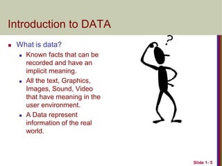
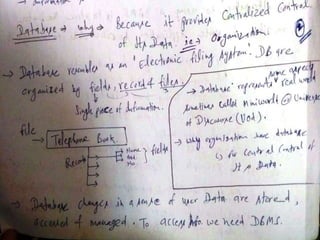
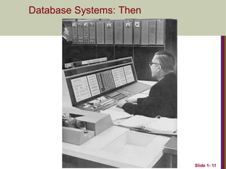

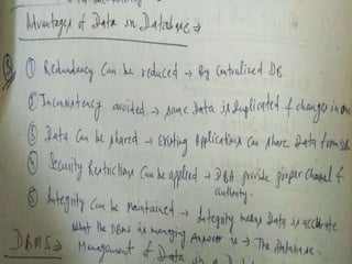
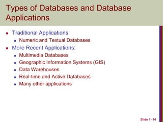
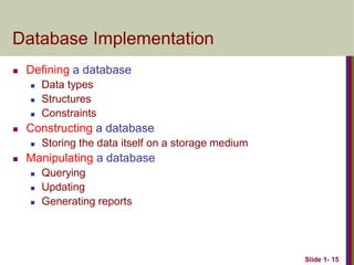
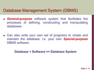
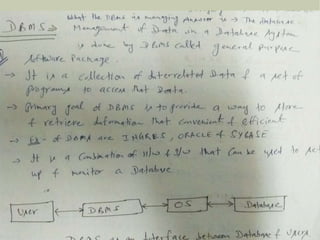
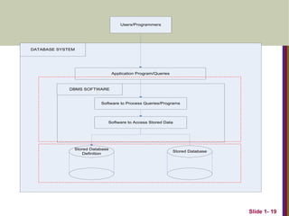
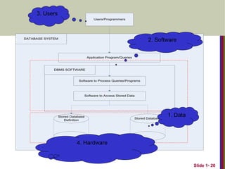
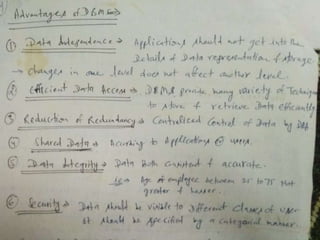
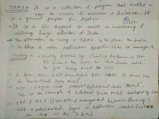
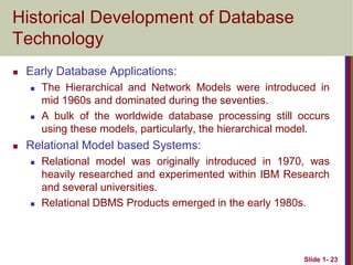
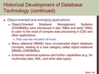
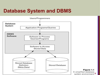
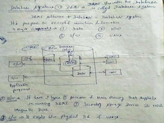
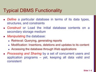
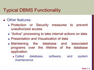
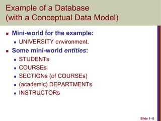
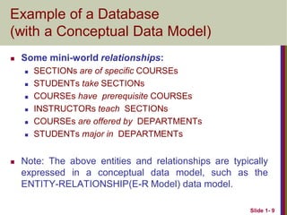
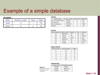
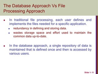
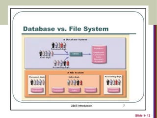
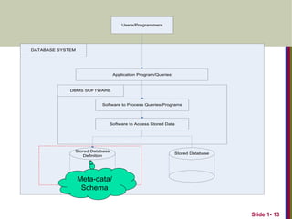
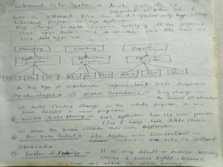
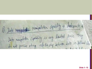
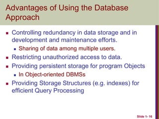
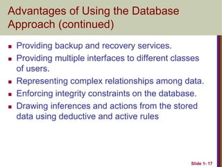
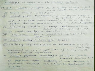

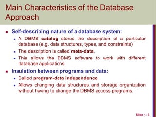
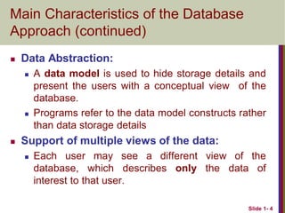
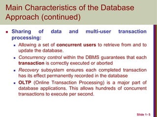
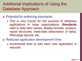
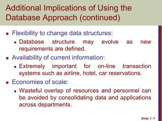
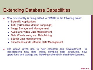
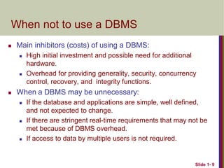
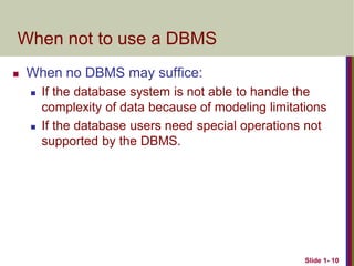
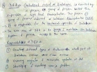
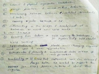

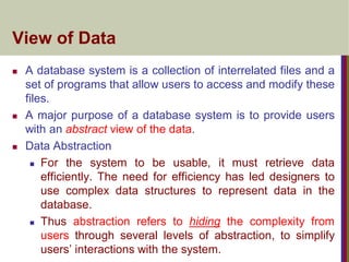
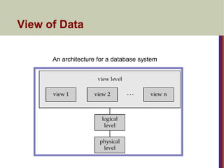
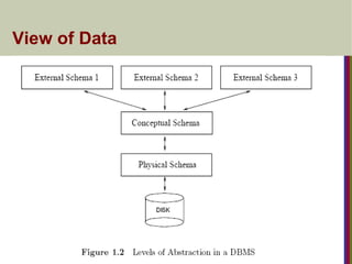
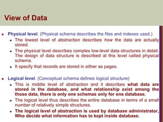
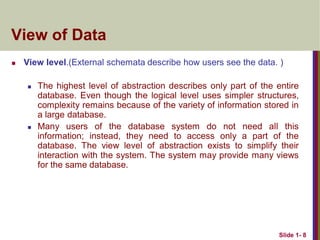
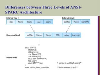
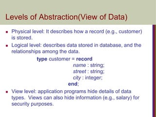
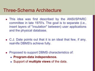
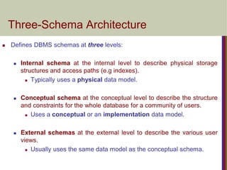
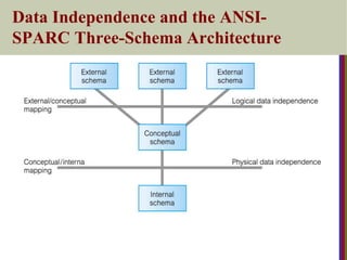
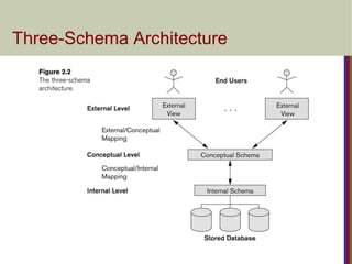

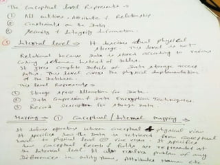
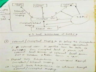

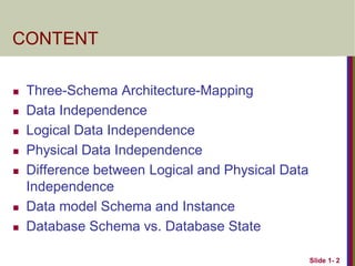
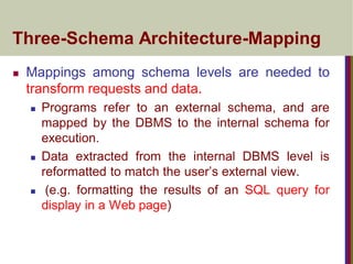
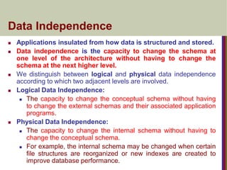
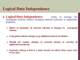
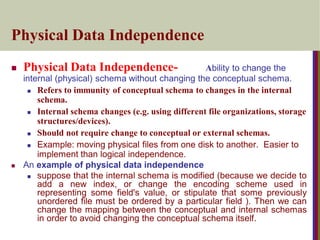
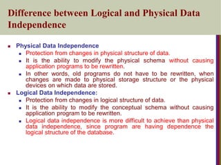
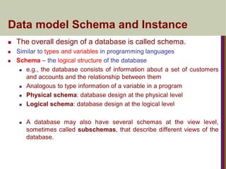
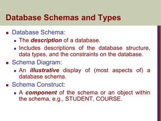
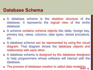
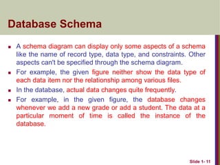
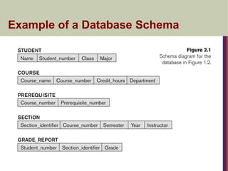
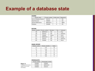

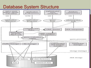
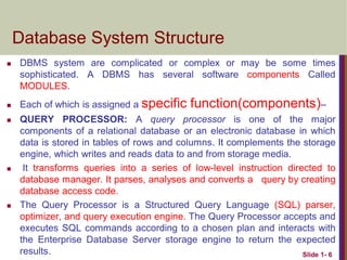
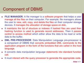
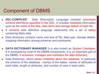
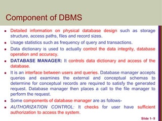
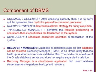
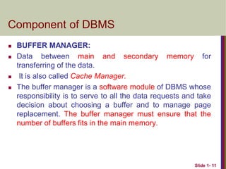
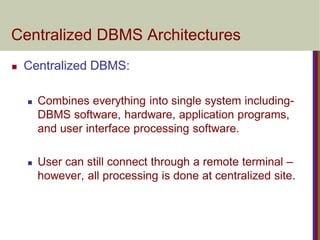
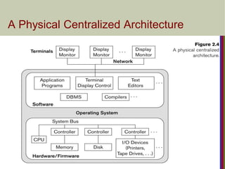

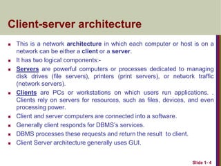
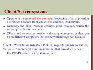
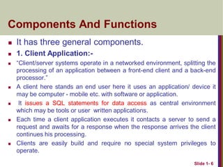

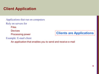
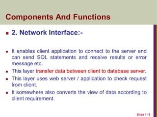
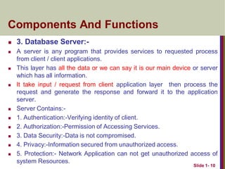
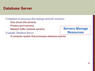

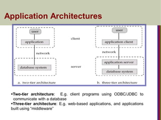
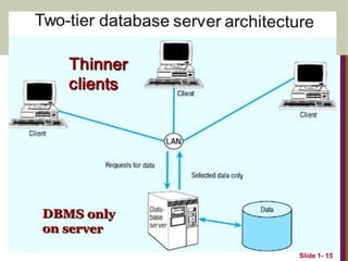
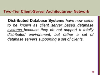
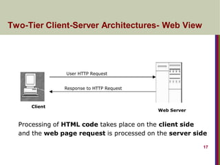
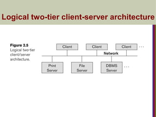
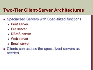
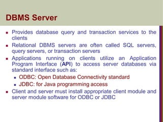
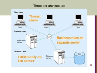
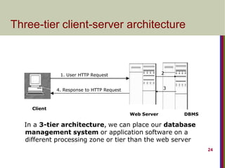
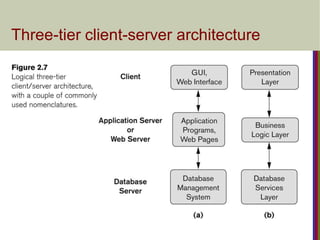
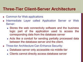
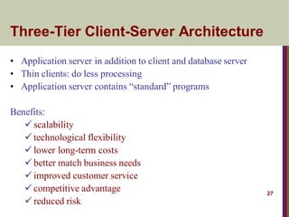
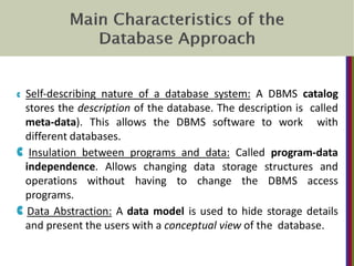
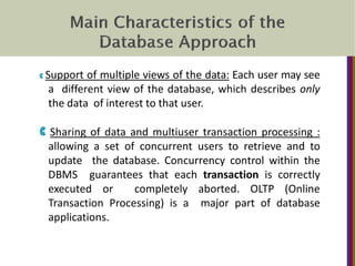
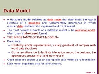
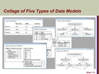
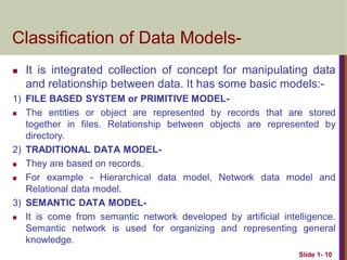
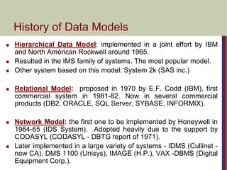
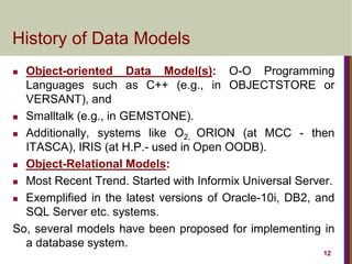
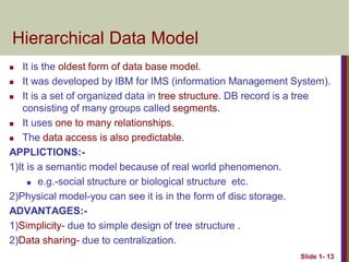
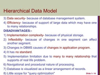
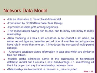
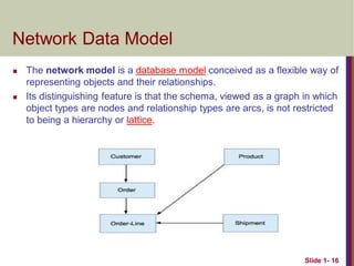
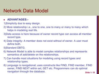
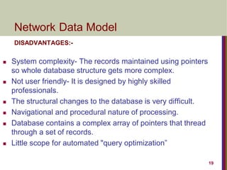


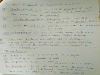
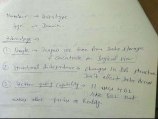
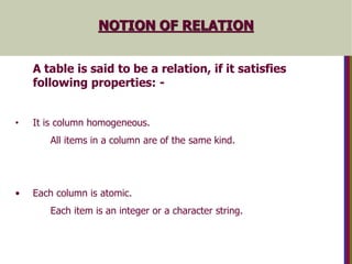
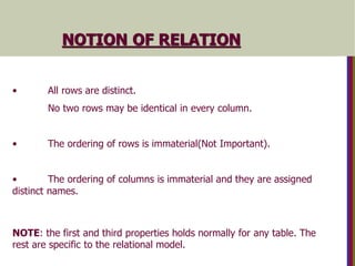
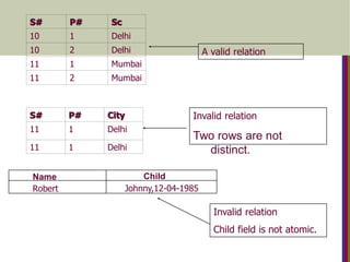

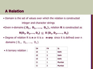
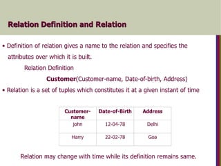
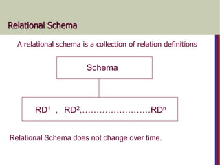
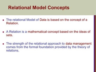
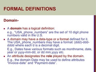
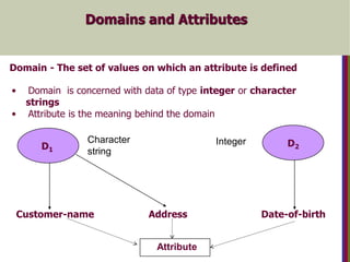
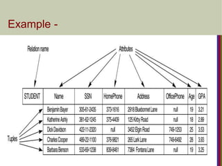
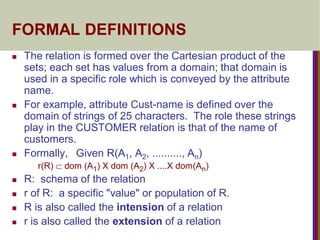
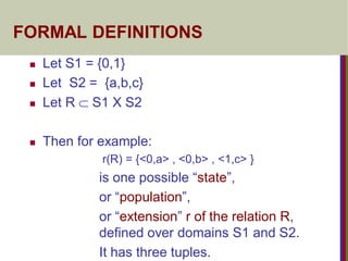
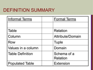
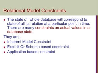
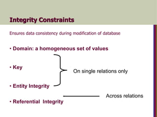
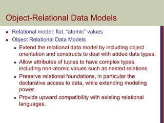
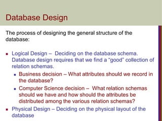
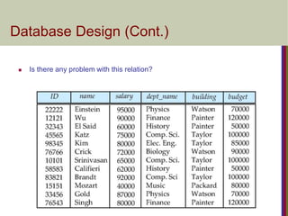
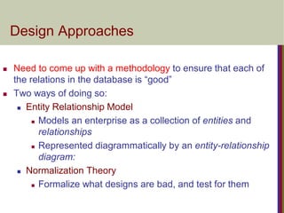

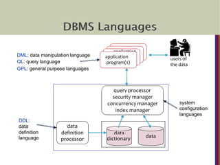
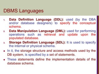
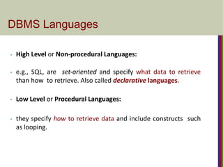
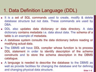
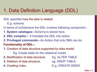
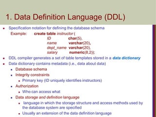
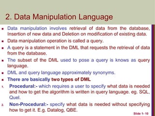
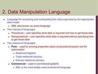
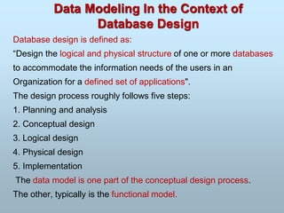

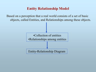

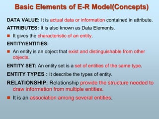
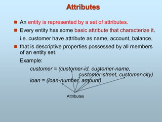
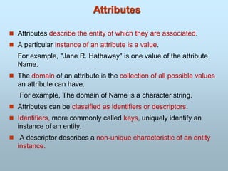
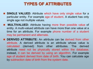
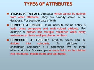
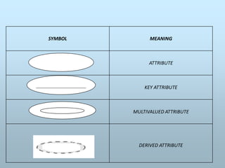
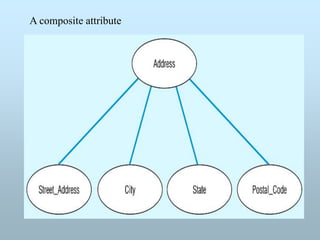
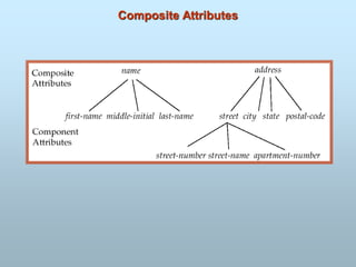
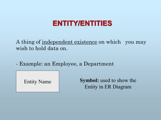
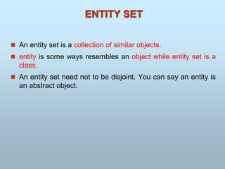
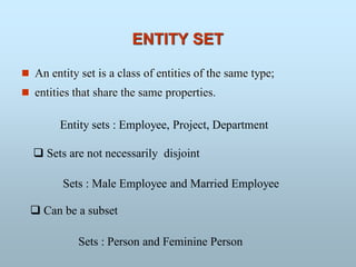
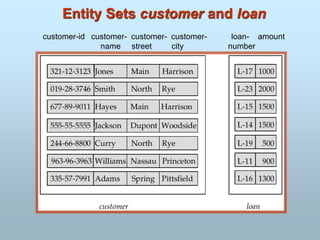
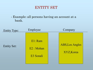
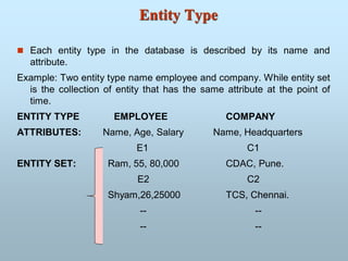
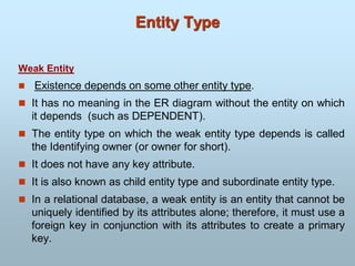
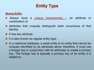
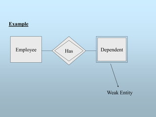
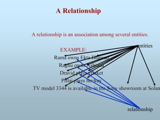

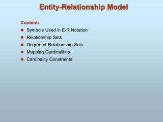
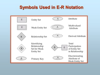
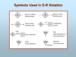
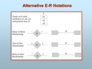
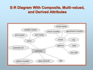
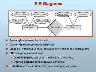
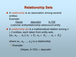
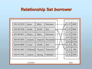
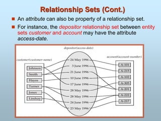
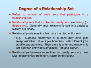
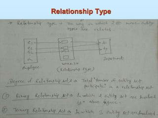
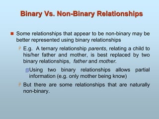
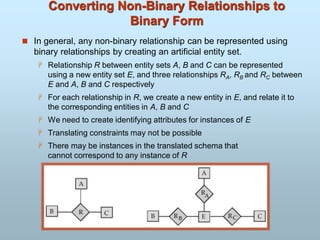
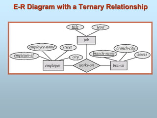
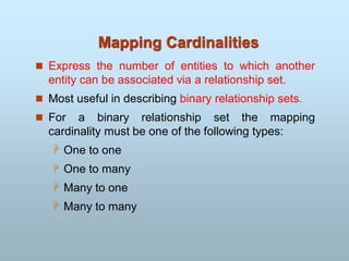

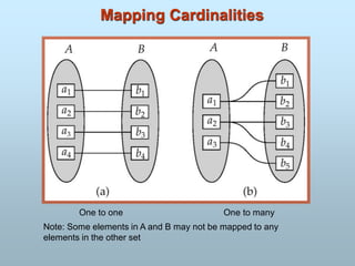
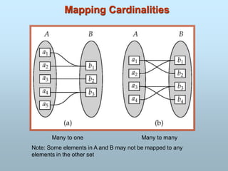
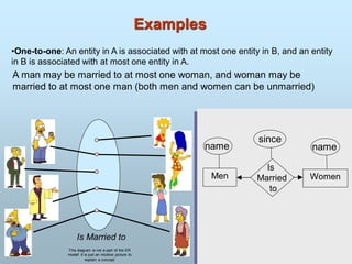
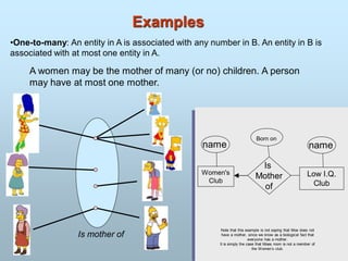
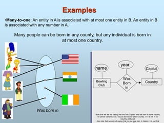
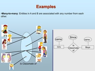
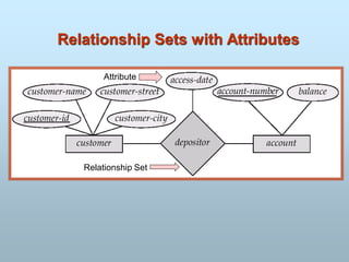
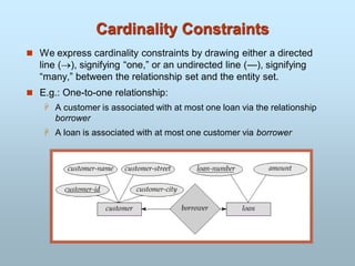
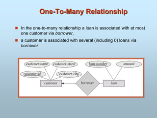
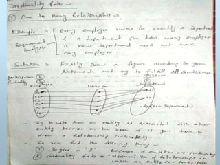
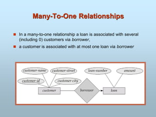
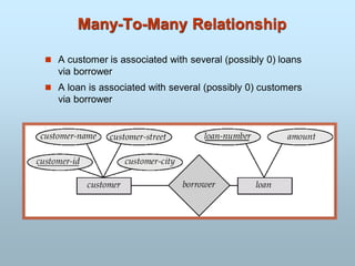
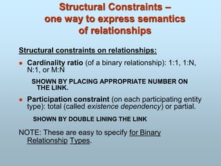
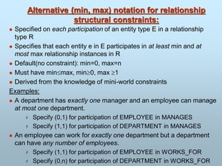
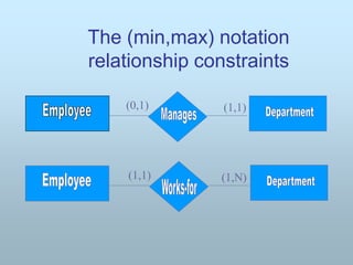

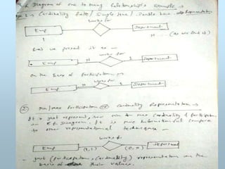

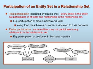
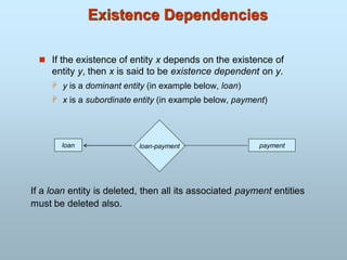
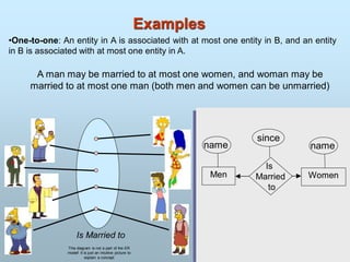
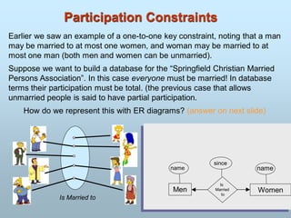
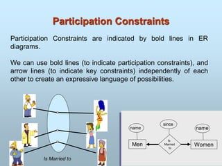
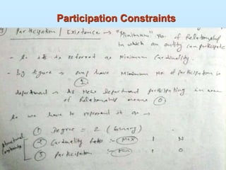
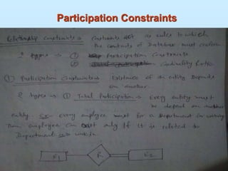
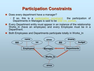
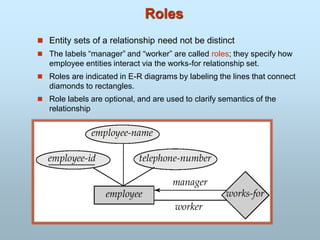
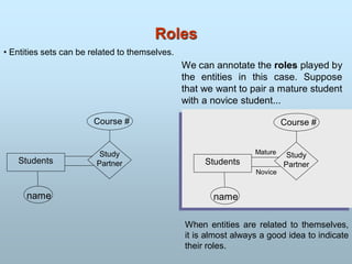

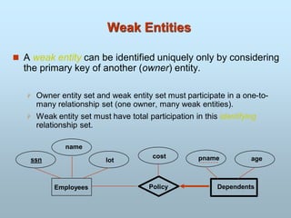
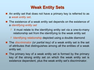
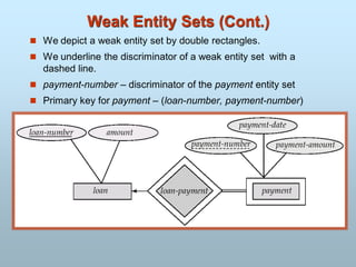
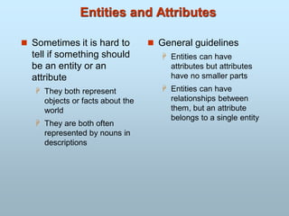
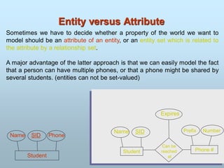
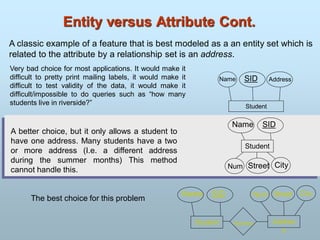
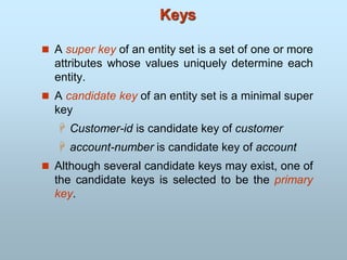
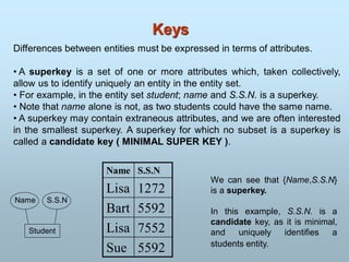
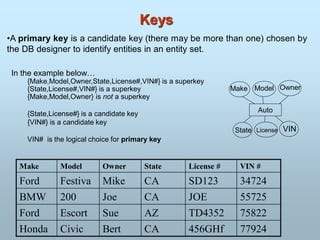

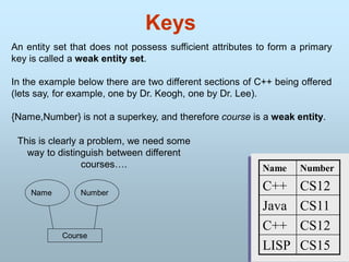
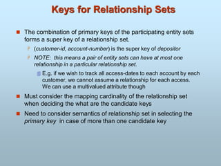

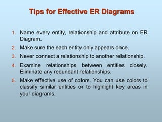
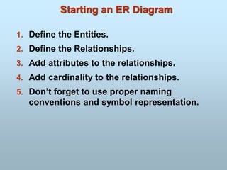
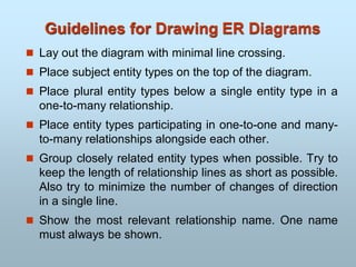
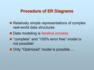
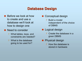
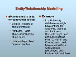
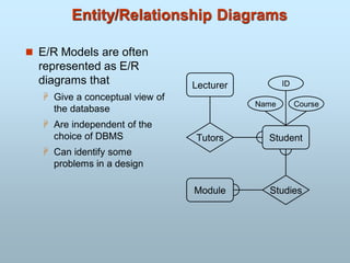
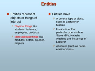
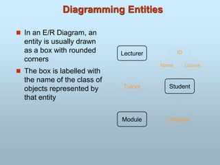
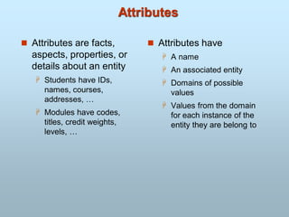
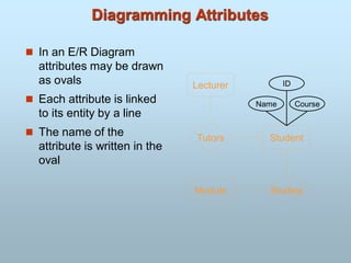
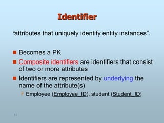
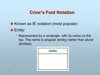
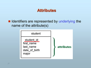

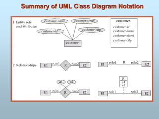
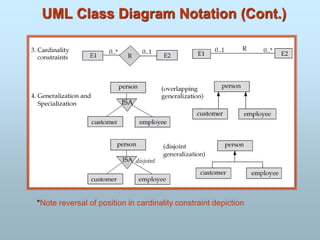
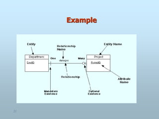
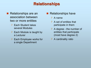
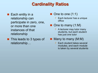
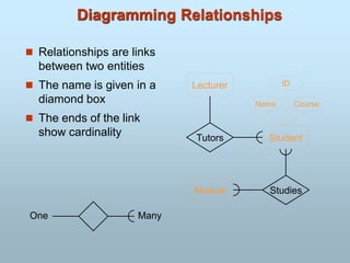

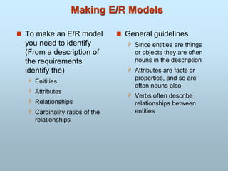
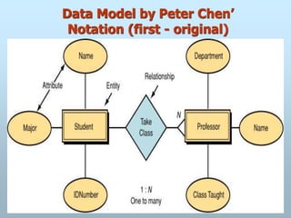

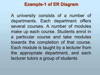
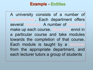
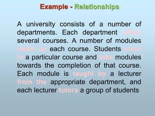
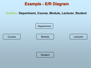
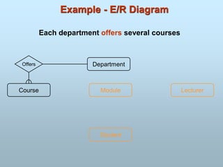
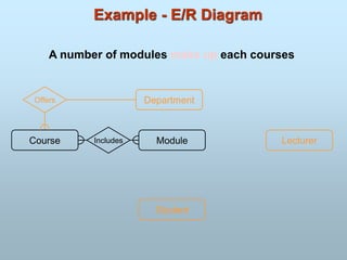
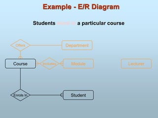
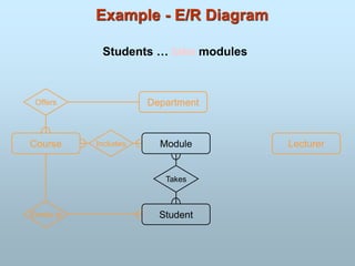
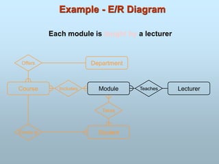
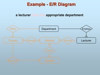
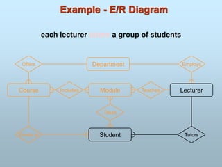
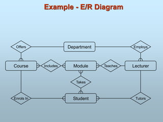

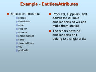
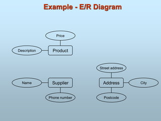
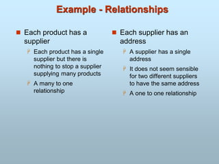
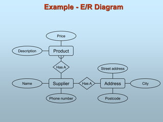
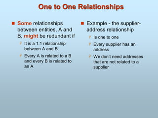
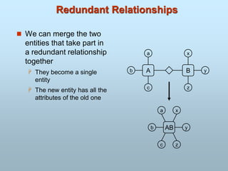
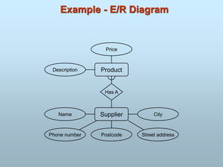
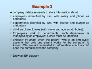
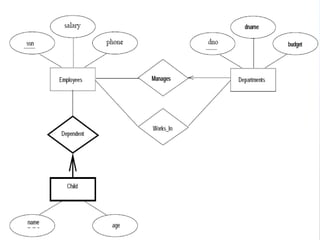
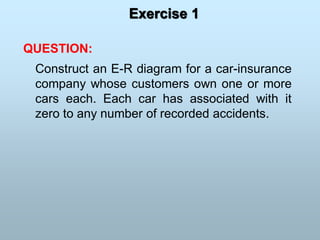
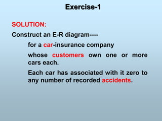
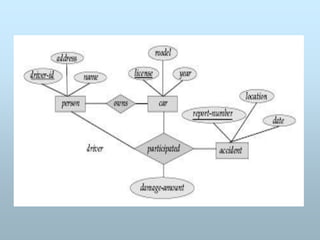
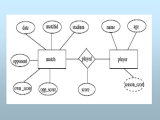
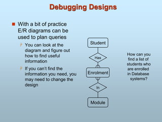
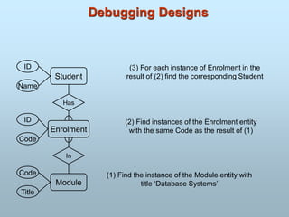
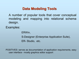
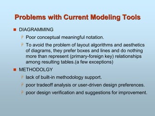
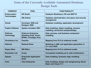


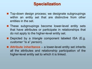
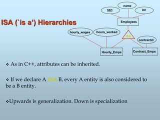
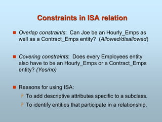
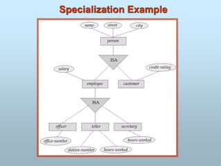
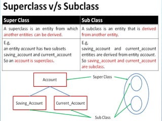
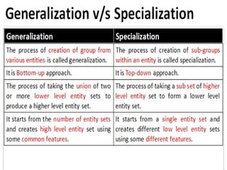
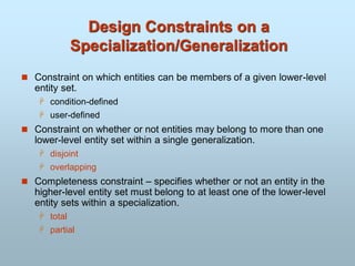
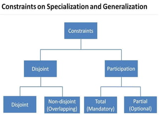
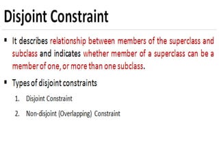
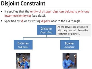
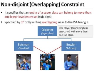
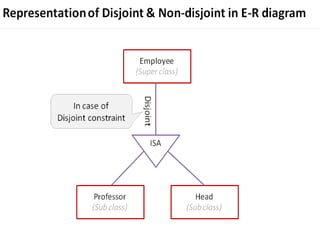
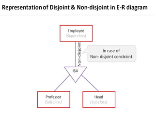
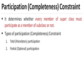
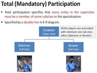
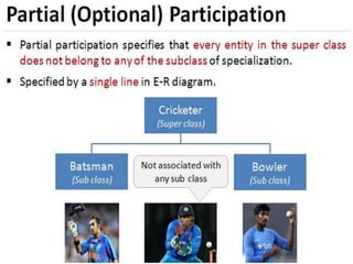
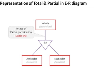
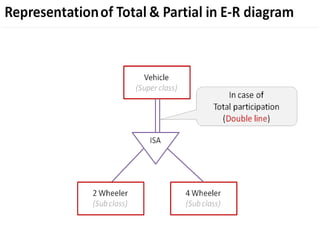
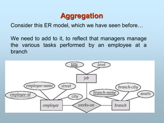
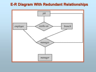
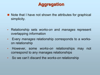
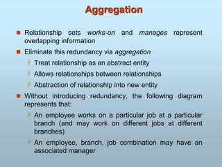
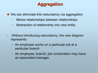
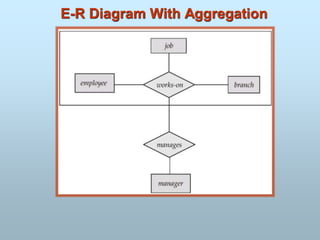
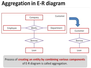
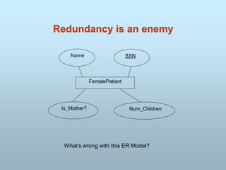

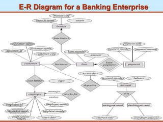
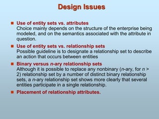
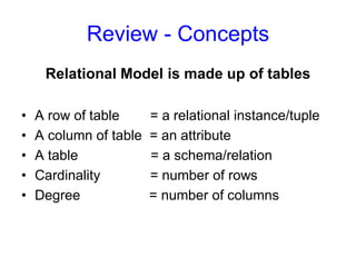
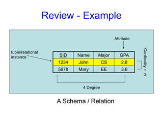
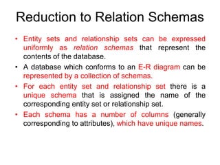
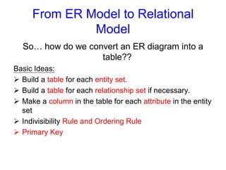
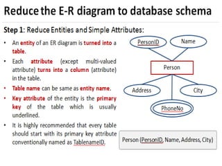
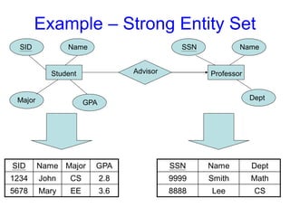
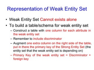
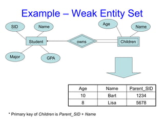
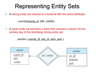
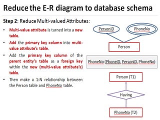
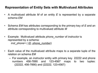
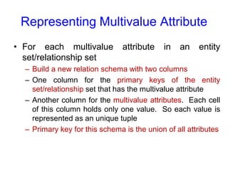
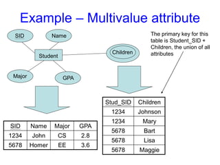
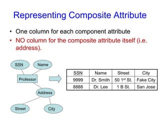
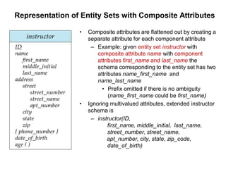
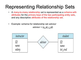
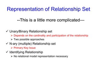
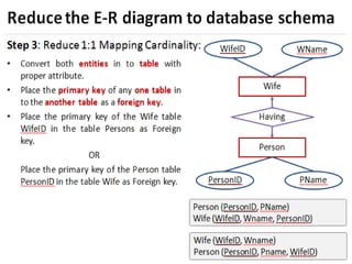
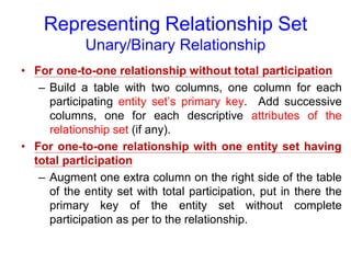
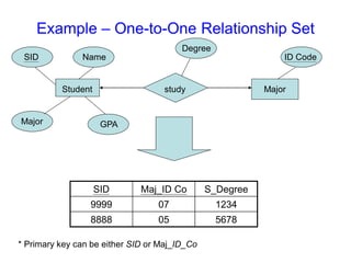
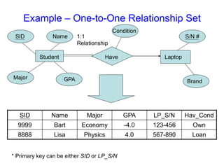
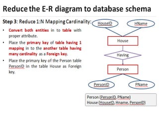
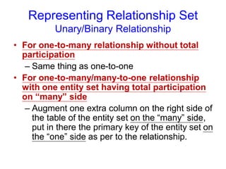
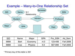
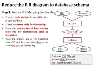
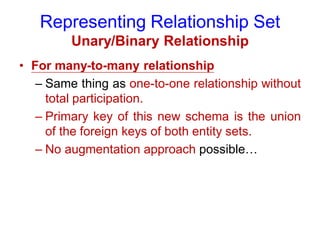
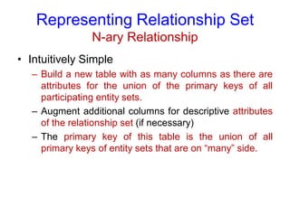
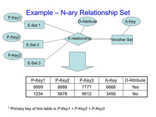
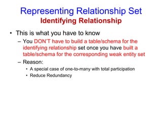
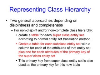
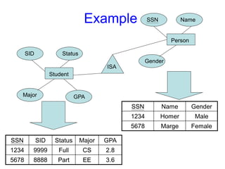
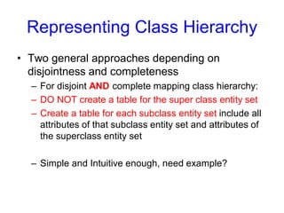
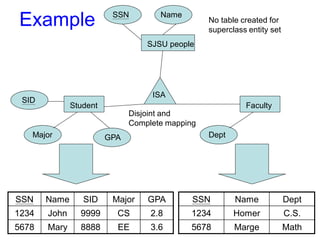
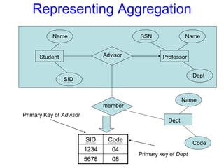
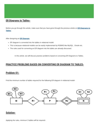
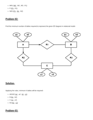
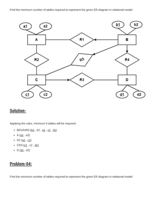
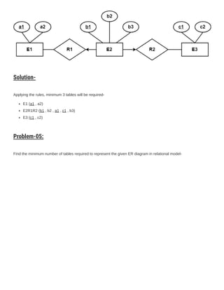
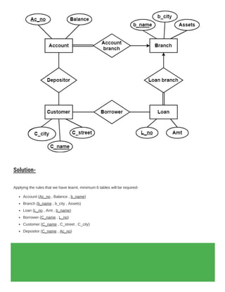
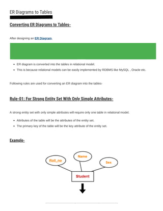
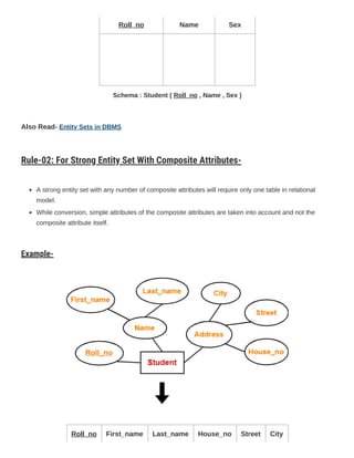
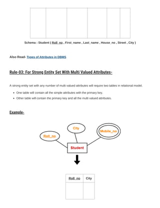
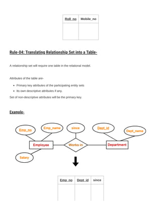
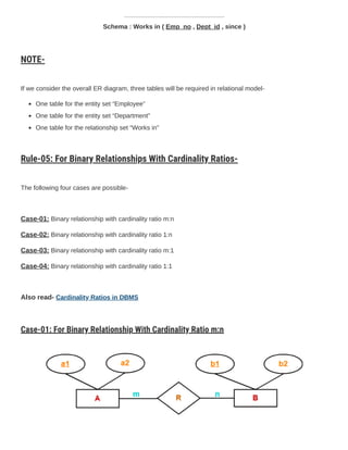
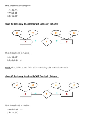
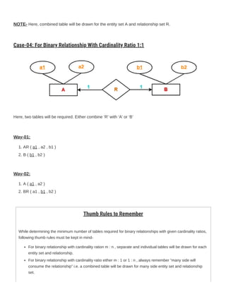
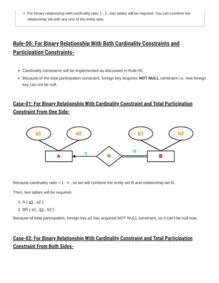
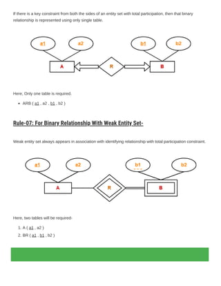
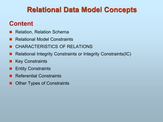
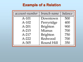
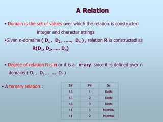
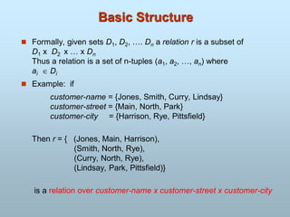
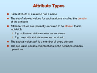
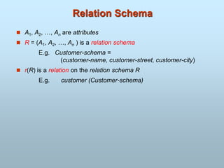
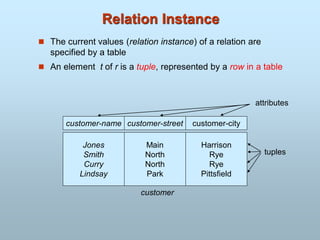
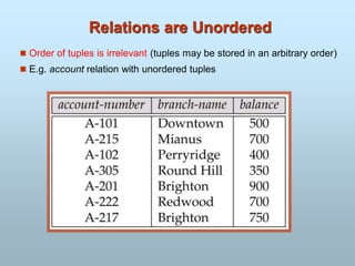
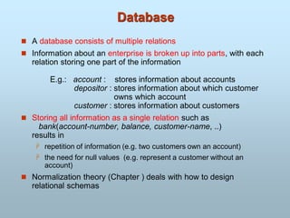
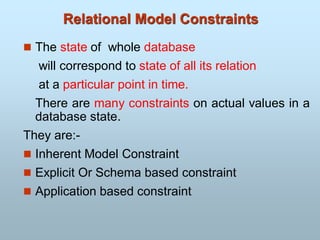
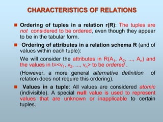
![CHARACTERISTICS OF RELATIONS
Notation:
- We refer to component values of a tuple t by
t[Ai] = vi (the value of attribute Ai for tuple t).
Similarly, t[Au, Av, ..., Aw] refers to the subtuple of t
containing the values of attributes Au, Av, ..., Aw,
respectively.](https://image.slidesharecdn.com/dbmscombine-251224035216-cbcde31f/85/dbms-combine-with-sql-for-engineering-pdf-451-320.jpg)
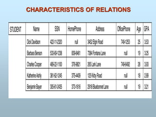
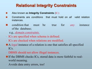
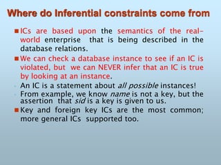
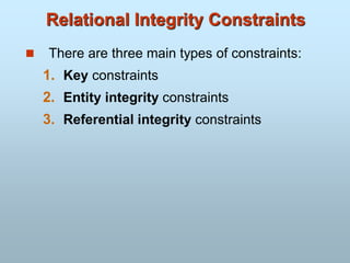
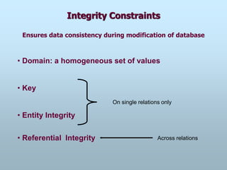
![Concept of Key
• Relation is a set of distinct tuples.
• Find a minimal set of attributes denoted by K such that for every pair of
tuples t1,t2
t1[K] t2 [K]
• K is known as key of relation R.
A minimal set
If (a, b, c, d…) is a key then no proper subset of it is a key as well](https://image.slidesharecdn.com/dbmscombine-251224035216-cbcde31f/85/dbms-combine-with-sql-for-engineering-pdf-457-320.jpg)
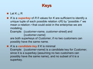
![Key Constraints
Superkey of R: A set of attributes SK of R such that no
two tuples in any valid relation instance r(R) will have
the same value for SK. That is, for any distinct tuples t1
and t2 in r(R), t1[SK] t2[SK].
Key of R: A "minimal" superkey; that is, a superkey K
such that removal of any attribute from K results in a set
of attributes that is not a superkey.
Example: The CAR relation schema:
CAR(State, Reg#, SerialNo, Make, Model, Year)
has two keys Key1 = {State, Reg#}, Key2 = {SerialNo}, which are also
superkeys. {SerialNo, Make} is a superkey but not a key.
If a relation has several candidate keys, one is chosen
arbitrarily to be the primary key. The primary key
attributes are underlined.](https://image.slidesharecdn.com/dbmscombine-251224035216-cbcde31f/85/dbms-combine-with-sql-for-engineering-pdf-459-320.jpg)
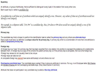
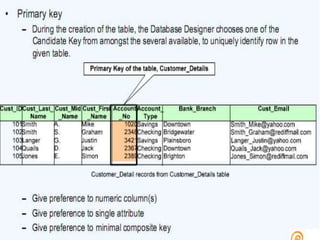
![Entity Integrity
Relational Database Schema: A set S of relation
schemas that belong to the same database. S is the name
of the database.
S = {R1, R2, ..., Rn}
Entity Integrity: The primary key attributes PK of each
relation schema R in S cannot have null values in any tuple
of r(R). This is because primary key values are used to
identify the individual tuples.
t[PK] null for any tuple t in r(R)
Note: Other attributes of R may be similarly constrained
to disallow null values, even though they are not members
of the primary key.](https://image.slidesharecdn.com/dbmscombine-251224035216-cbcde31f/85/dbms-combine-with-sql-for-engineering-pdf-462-320.jpg)
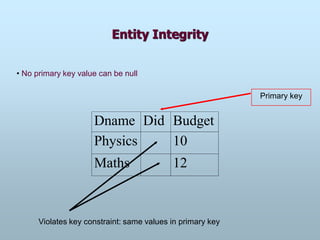
![Referential Integrity
A constraint involving two relations (the previous
constraints involve a single relation).
Used to specify a relationship among tuples in two
relations: the referencing relation and the referenced
relation.
Tuples in the referencing relation R1 have attributes FK
(called foreign key attributes) that reference the
primary key attributes PK of the referenced relation R2.
A tuple t1 in R1 is said to reference a tuple t2 in R2 if
t1[FK] = t2[PK].
A referential integrity constraint can be displayed in a
relational database schema as a directed arc from
R1.FK to R2.](https://image.slidesharecdn.com/dbmscombine-251224035216-cbcde31f/85/dbms-combine-with-sql-for-engineering-pdf-464-320.jpg)
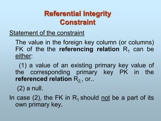
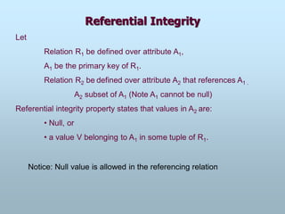
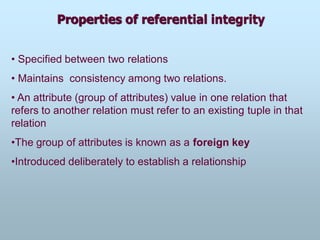
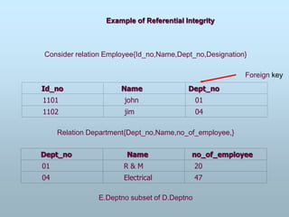
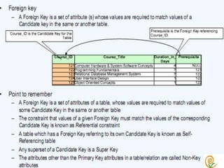
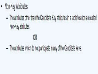
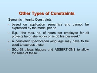
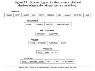
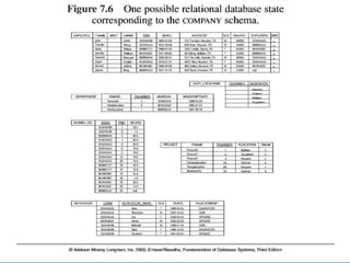
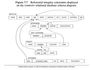
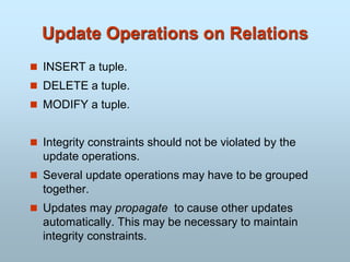
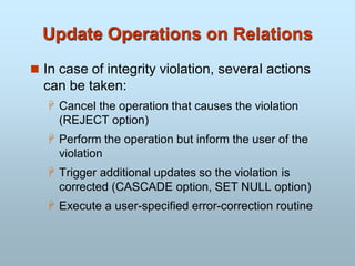
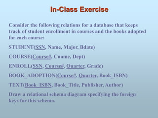
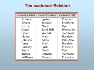
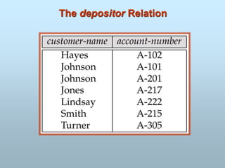
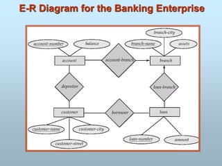
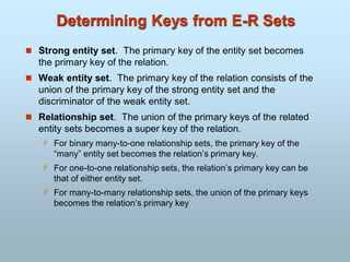
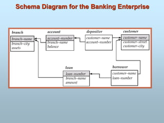
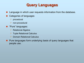
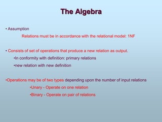
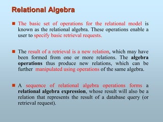
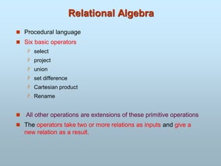
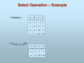
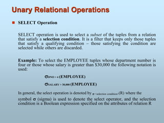
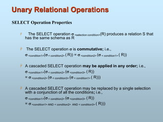
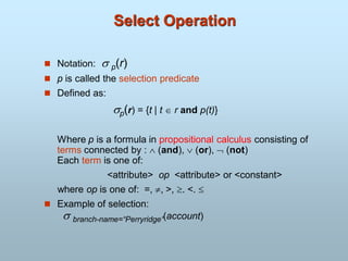
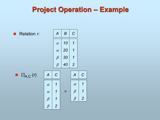
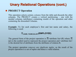
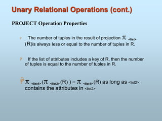
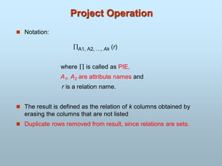
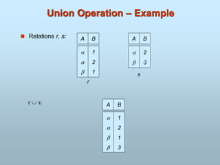
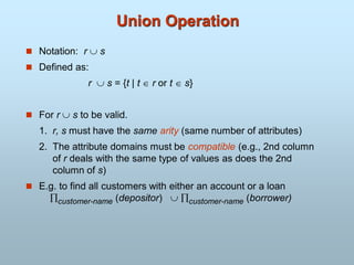
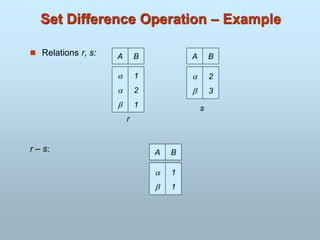
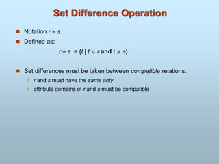

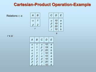
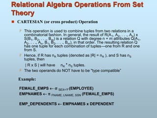
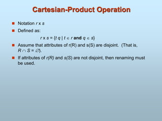
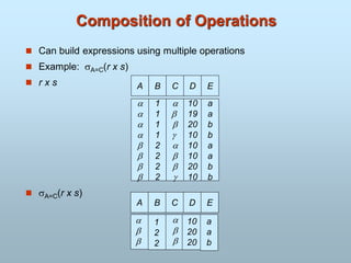
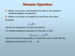
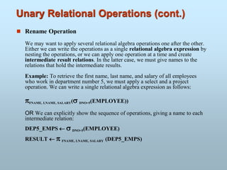
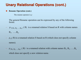
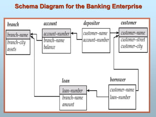
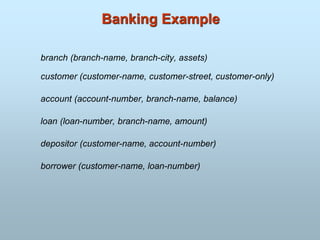
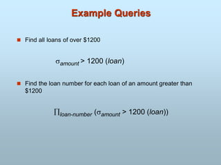
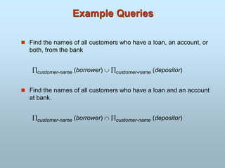
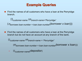
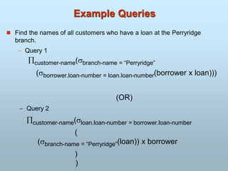
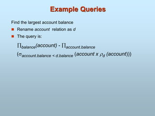
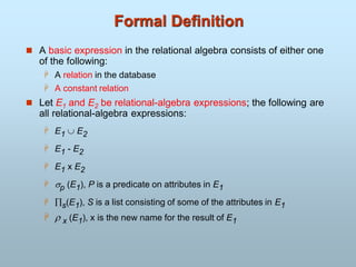
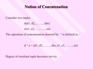
![CROSS PRODUCT
Let there be relations R(A1, A2, …., An) and S(B1, B2,….Bm)
then
R X S = {(r ^ s) : r ε R and s ε S}
Therefore Z = R X S = Z(A1, A2, …., An, B1, ….Bm)
Z contains all tuples t for which
there is a tuple t1 in R and t2 in S
for which t[A1,… An]=t1[A1,…An] and
t[B1,… Bm]= t2[B1,…Bm]](https://image.slidesharecdn.com/dbmscombine-251224035216-cbcde31f/85/dbms-combine-with-sql-for-engineering-pdf-518-320.jpg)

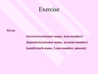
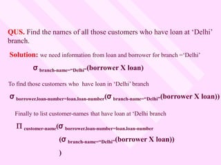
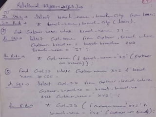
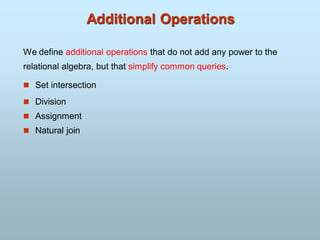
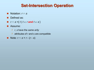
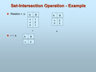
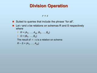
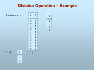
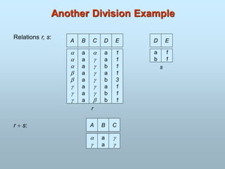
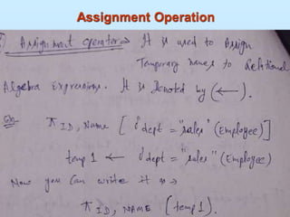
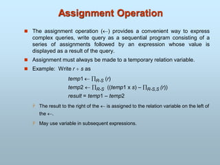
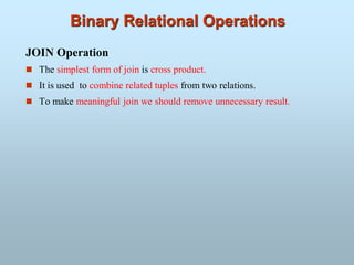
![JOIN Operation
Define join, also called θ-join, of R and S on attributes A and B as :
RA θ B S = { r ^ s : r ε R, s ε S and (r[A] θ s[B] )}
where domains of A and B are union compatible.
When θ is =, join is said to be equi-join
•The generalised join If R(A1,A2,…….,An) and S(B1, B2, ….., Bm), then
the generalised join is Z (A1, A2,……., An, B1, B2, ….., Bm)
•The natural join : A generalised join but with the common attribute
occurring only once. Most usually used
• The composed join : It is a natural join with the domains on which join
occurred removed.](https://image.slidesharecdn.com/dbmscombine-251224035216-cbcde31f/85/dbms-combine-with-sql-for-engineering-pdf-533-320.jpg)
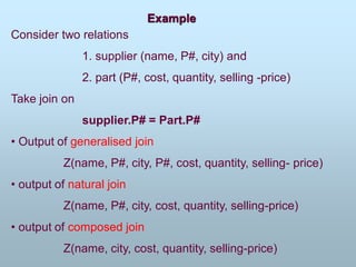
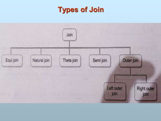
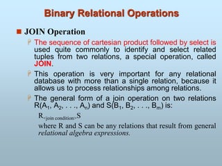
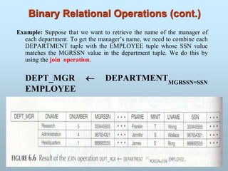
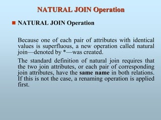
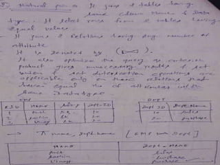
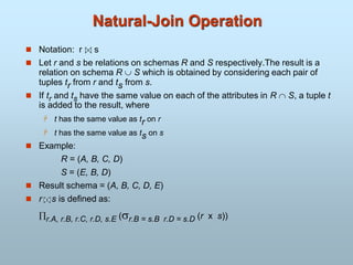
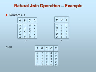
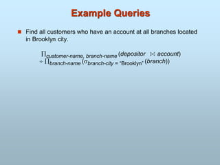
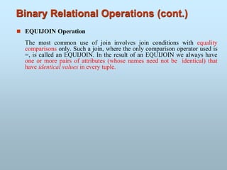
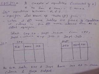
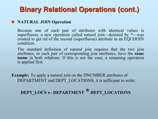
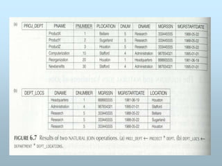
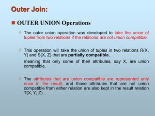
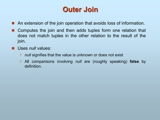
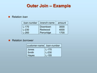
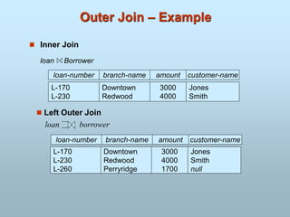
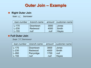
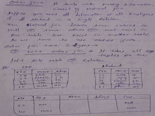
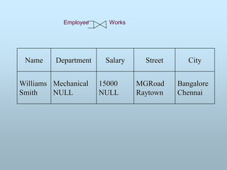
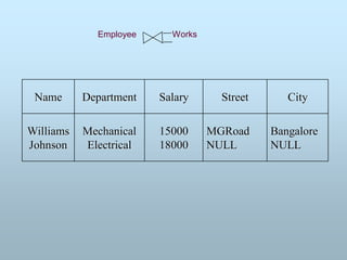
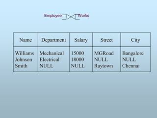
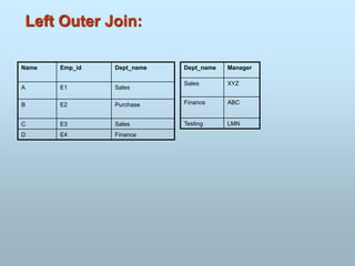
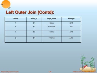
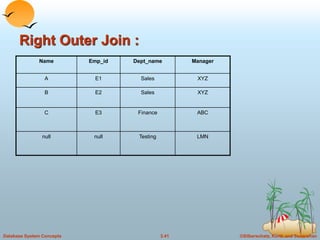
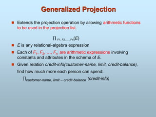
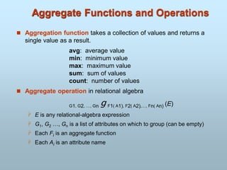
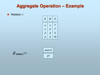
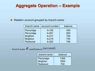
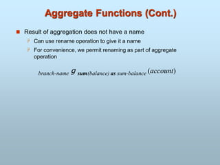
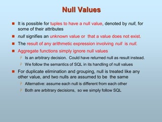
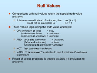
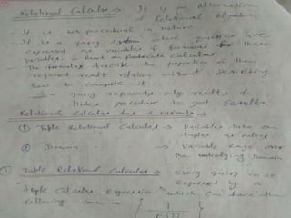
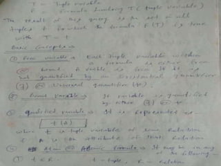
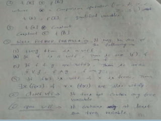
![Tuple Relational Calculus
Introduced by E.F. CODD
Declarative database query language.
Nonprocedural query language.
A nonprocedural query language, where each query is of the form
{t | P (t) }
It is the set of all tuples t such that predicate P is true for t
t is a tuple variable, t[A] denotes the value of tuple t on attribute A
t r denotes that tuple t is in relation r
P is a formula similar to that of the predicate calculus](https://image.slidesharecdn.com/dbmscombine-251224035216-cbcde31f/85/dbms-combine-with-sql-for-engineering-pdf-570-320.jpg)
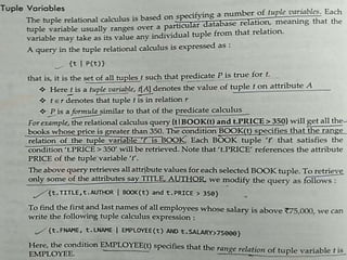
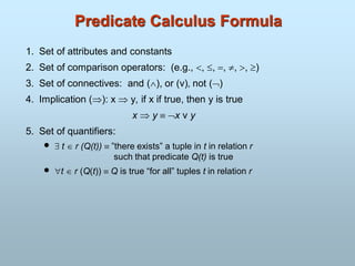
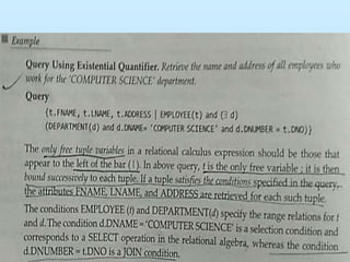
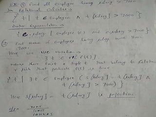
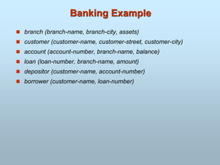
![Example Queries
Find the loan-number, branch-name, and amount for loans of
over $1200.
{t | t loan t [amount] 1200}
Find the loan number for each loan of an amount greater than
$1200
{t | s loan (t[loan-number] = s[loan-number]
s [amount] 1200}
Notice that a relation on schema [customer-name] is implicitly
defined by the query](https://image.slidesharecdn.com/dbmscombine-251224035216-cbcde31f/85/dbms-combine-with-sql-for-engineering-pdf-576-320.jpg)
![Example Queries
Find the names of all customers having a loan, an account, or both
at the bank
{t | s borrower(t[customer-name] = s[customer-name])
u depositor(t[customer-name] = u[customer-name])
Find the names of all customers who have a loan and an account
at the bank
{t | s borrower(t[customer-name] = s[customer-name])
u depositor(t[customer-name] = u[customer-name])](https://image.slidesharecdn.com/dbmscombine-251224035216-cbcde31f/85/dbms-combine-with-sql-for-engineering-pdf-577-320.jpg)
![Example Queries
Find the names of all customers having a loan at the Perryridge
branch
{t | s borrower(t[customer-name] = s[customer-name]
u loan(u[branch-name] = “Perryridge”
u[loan-number] = s[loan-number]))}
Find the names of all customers who have a loan at the
Perryridge branch, but no account at any branch of the bank
{t | s borrower(t[customer-name] = s[customer-name]
u loan(u[branch-name] = “Perryridge”
u[loan-number] = s[loan-number]))
not v depositor (v[customer-name] =
t[customer-name]) }](https://image.slidesharecdn.com/dbmscombine-251224035216-cbcde31f/85/dbms-combine-with-sql-for-engineering-pdf-578-320.jpg)
![Example Queries
Find the names of all customers having a loan from the
Perryridge branch, and the cities they live in
{t | s loan(s[branch-name] = “Perryridge”
u borrower (u[loan-number] = s[loan-number]
t [customer-name] = u[customer-name])
v customer (u[customer-name] = v[customer-name]
t[customer-city] = v[customer-city])))}](https://image.slidesharecdn.com/dbmscombine-251224035216-cbcde31f/85/dbms-combine-with-sql-for-engineering-pdf-579-320.jpg)
![Example Queries
Find the names of all customers who have an account at all
branches located in Brooklyn:
{t | c customer (t[customer.name] = c[customer-name])
s branch(s[branch-city] = “Brooklyn”
u account ( s[branch-name] = u[branch-name]
s depositor ( t[customer-name] = s[customer-name]
s[account-number] = u[account-number] )) )}](https://image.slidesharecdn.com/dbmscombine-251224035216-cbcde31f/85/dbms-combine-with-sql-for-engineering-pdf-580-320.jpg)
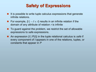
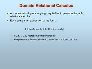
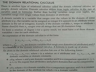
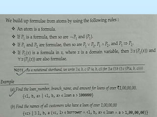
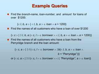
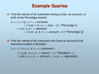
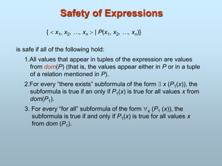
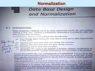
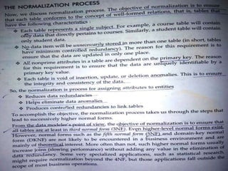
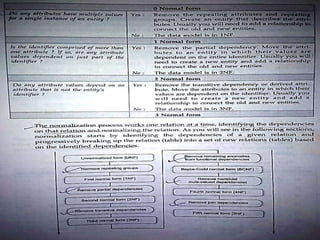
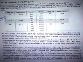
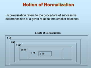
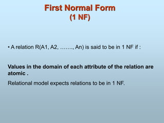
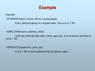
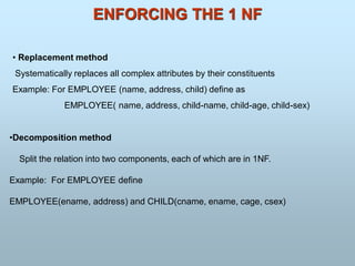
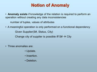
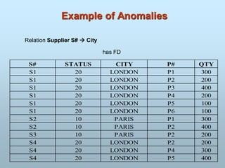
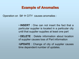
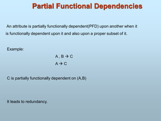
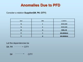
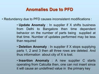
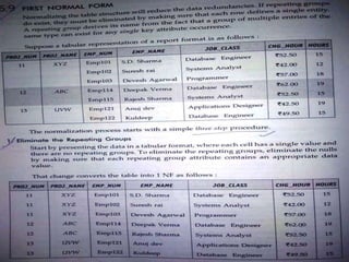
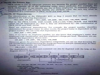

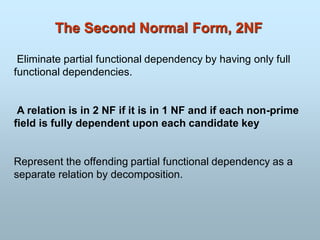
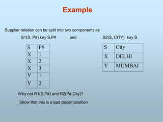
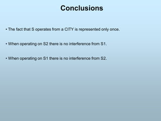
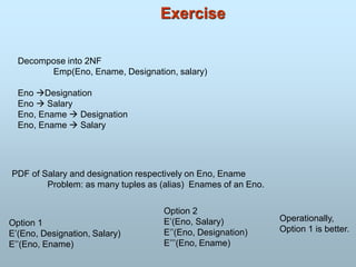
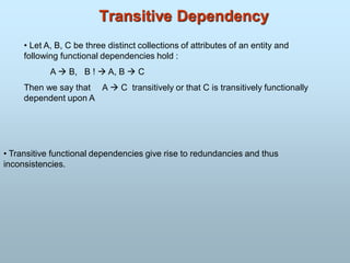
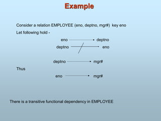
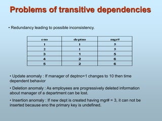


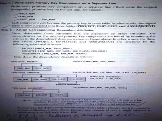
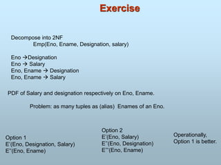
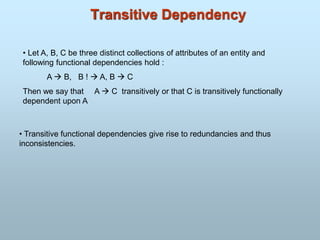

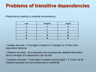
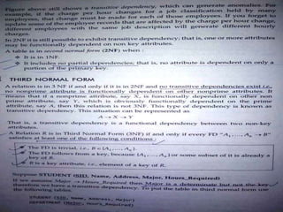
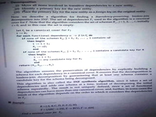

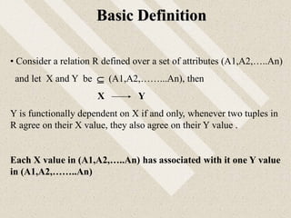
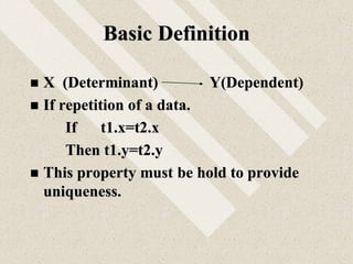
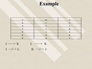
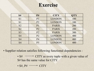
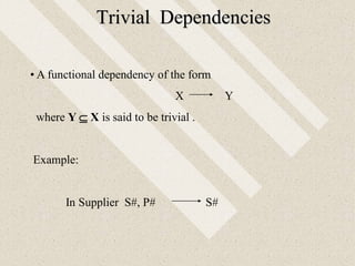
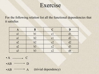
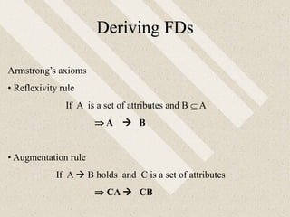
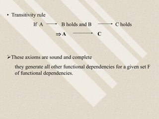
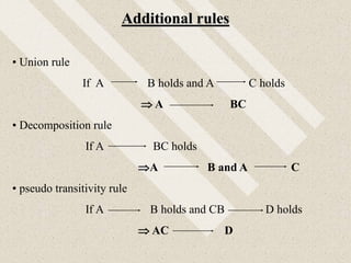
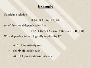
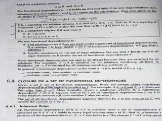
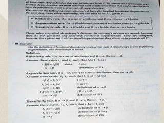
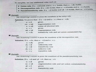
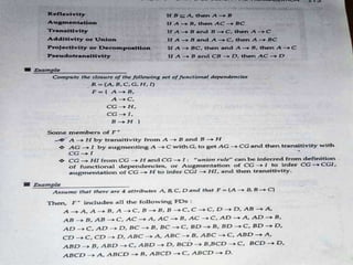
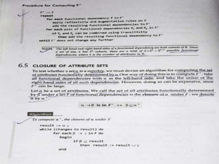
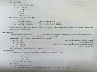
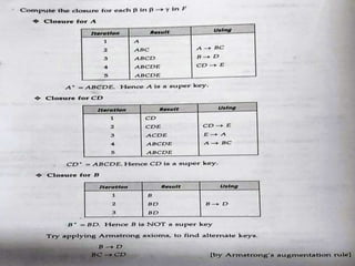
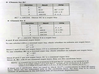
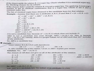
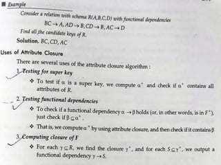

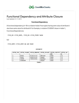
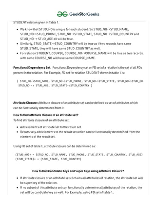
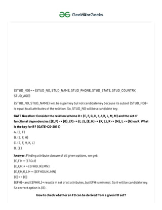
![To check whether an FD A->B can be derived from an FD set F
,
1. Find (A)+ using FD set F
.
2. If B is subset of (A)+, then A->B is true else not true.
GATE Question: In a schema with attributes A, B, C, D and E following set of functional
dependencies are given
{A -> B, A -> C, CD -> E, B -> D, E -> A}
Which of the following functional dependencies is NOT implied by the above set? (GATE IT
2005)
A. CD -> AC
B. BD -> CD
C. BC -> CD
D. AC -> BC
Answer: Using FD set given in question,
(CD)+ = {CDEAB} which means CD -> AC also holds true.
(BD)+ = {BD} which means BD -> CD can’t hold true. So this FD is no implied in FD set. So (B) is the
required option.
Others can be checked in the same way.
Prime and non-prime attributes
Attributes which are parts of any candidate key of relation are called as prime attribute, others are
non-prime attributes. For Example, STUD_NO in STUDENT relation is prime attribute, others are
non-prime attribute.
GATE Question: Consider a relation scheme R = (A, B, C, D, E, H) on which the following
functional dependencies hold: {A–>B, BC–> D, E–>C, D–>A}. What are the candidate keys of R?
[GATE 2005]
(a) AE, BE
(b) AE, BE, DE
(c) AEH, BEH, BCH
(d) AEH, BEH, DEH
Answer: (AE)+ = {ABECD} which is not set of all attributes. So AE is not a candidate key. Hence
option A and B are wrong.
(AEH)+ = {ABCDEH}
(BEH)+ = {BEHCDA}
(BCH)+ = {BCHDA} which is not set of all attributes. So BCH is not a candidate key. Hence option C
](https://image.slidesharecdn.com/dbmscombine-251224035216-cbcde31f/85/dbms-combine-with-sql-for-engineering-pdf-651-320.jpg)
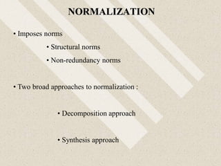
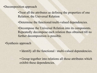
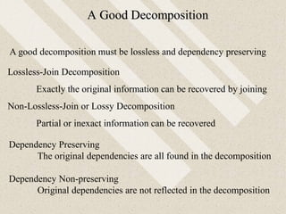
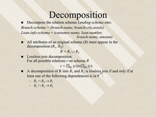
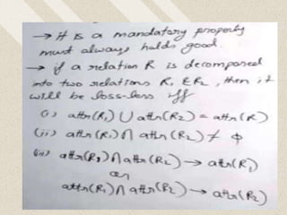
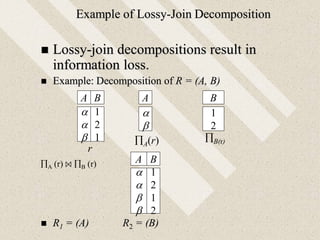
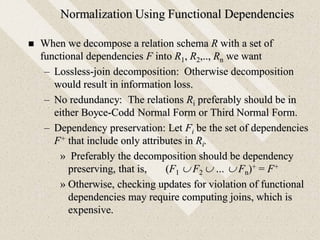
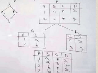
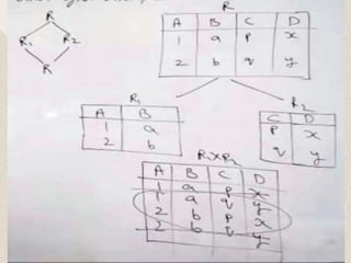
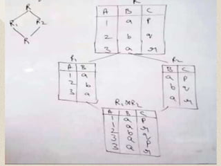
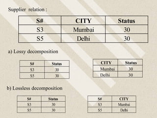
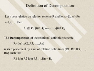
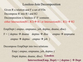
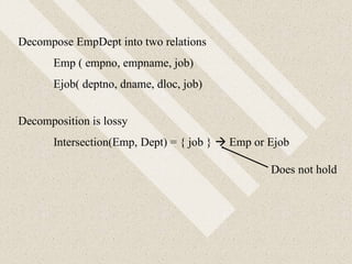
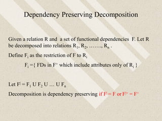
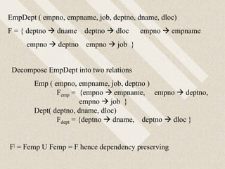
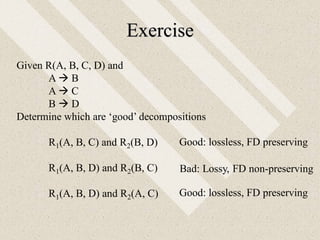
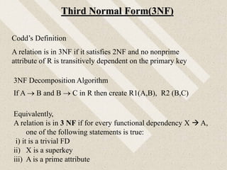
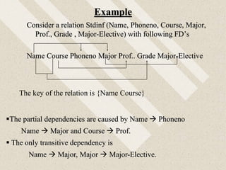
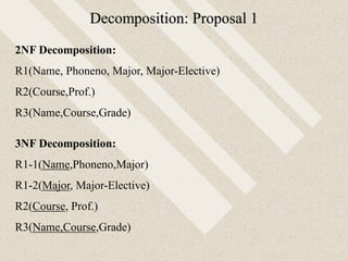
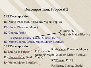

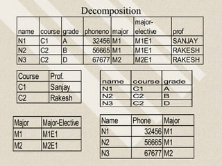
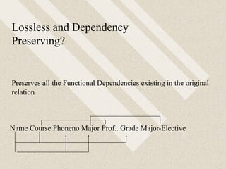
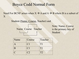
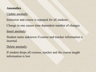
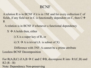
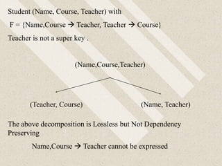
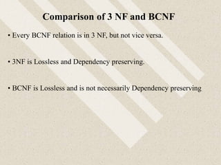
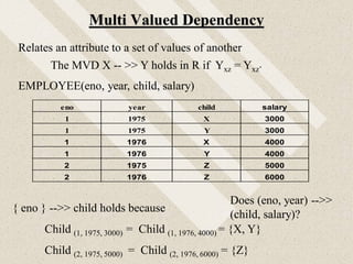
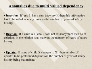
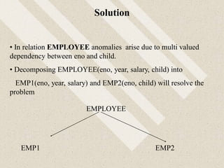
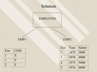
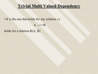
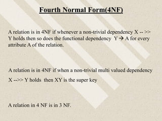
![The Fifth Normal Form
Concerned with eliminating Join Dependency
If a relation R is a join of certain of its projections then R exhibits
Join dependency
R satisfies JD *(X, Y, Z, …) iff R is join of R[X], R[Y], R[Z], …
Supply(Sno, Pno, Jobno) satisfies JD *([Sno, Pno], [Pno, Jobno],
[Sno, Jobno])
Sno Pno Jobno
S1 P1 J1
S1 P1 J2
S1 P2 J2
S2 P1 J2
JD *([Sno, Pno], [Pno, Jobno], [Sno, Jobno])
implies that supplier s supplies part p to a job j
only if
•s supplies p
•p is used in j
•s supplies to j](https://image.slidesharecdn.com/dbmscombine-251224035216-cbcde31f/85/dbms-combine-with-sql-for-engineering-pdf-692-320.jpg)
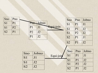
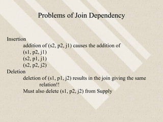
![Eliminating Problematic JDs
A JD is implied by candidate keys if every projection contains a
candidate key
JDs implied by candidate keys do not cause problems
Employee(Eno, Ename, Address) satisfies
JD *([Eno, Ename], [Eno, Address])
The candidate key Eno implies the JD
If Ename is also the candadate key then Ename implies
JD *([Eno, Ename], [Ename, Address])](https://image.slidesharecdn.com/dbmscombine-251224035216-cbcde31f/85/dbms-combine-with-sql-for-engineering-pdf-695-320.jpg)
![The Fifth Normal Form
A relation is in 5NF iff every join dependency is implied by the
candidate keys of R
Supply (Sno, Pno, Jobno) satisfies
JD *([Sno, Pno], [Pno, Jobno], [Sno, Jobno])
This JD is not implied by the candidate key
Decompose Supply into
SJ(Sno, Jobno), PJ(Pno, Jobno), SP(Sno, Pno)](https://image.slidesharecdn.com/dbmscombine-251224035216-cbcde31f/85/dbms-combine-with-sql-for-engineering-pdf-696-320.jpg)
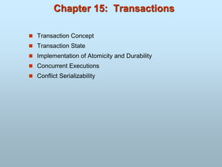
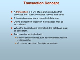
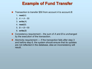
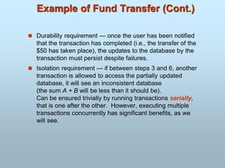
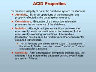
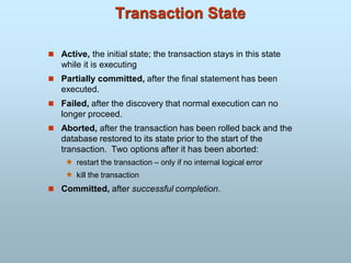
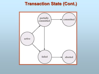
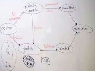
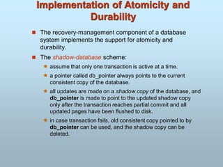
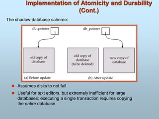
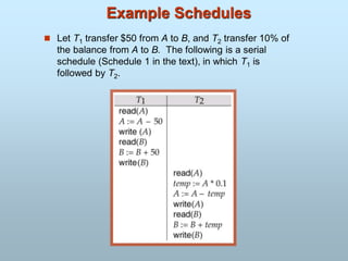
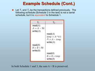
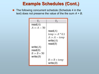
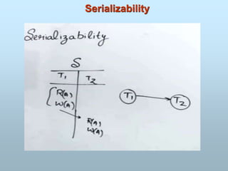
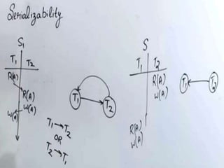
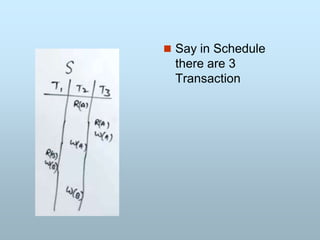
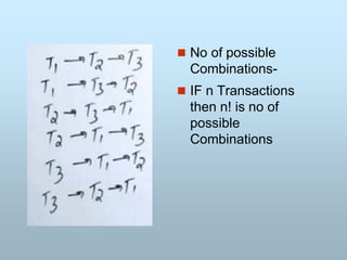
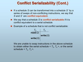
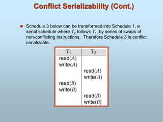
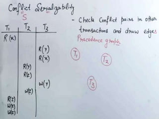
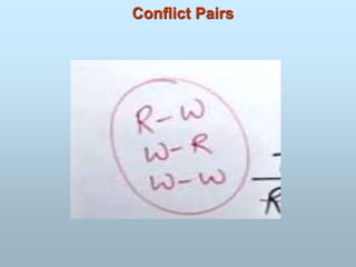
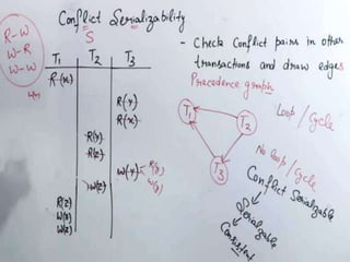
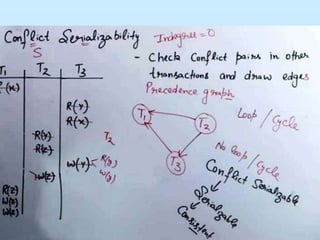
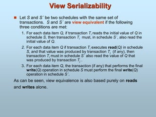
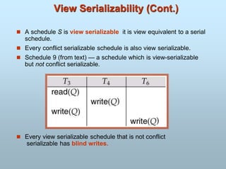
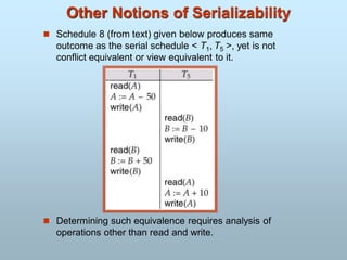
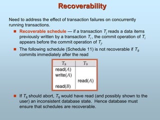
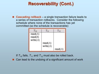
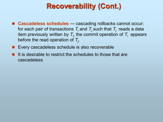
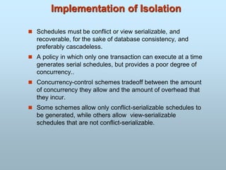
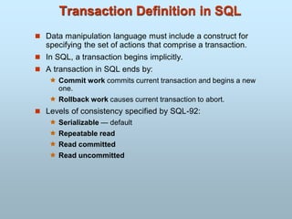
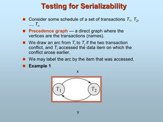
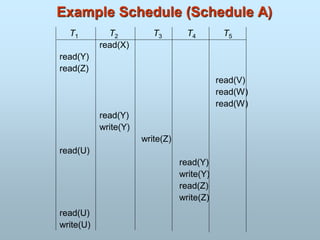
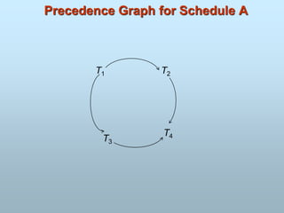
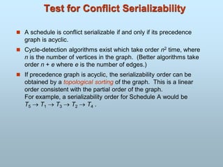


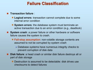
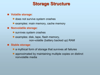
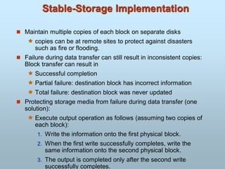
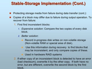
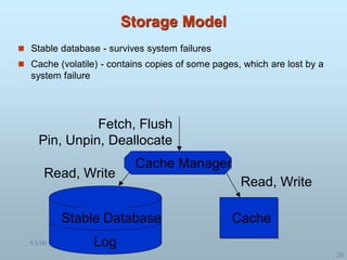
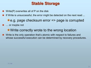
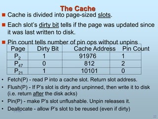
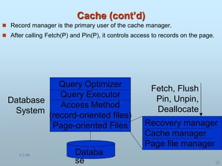
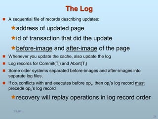
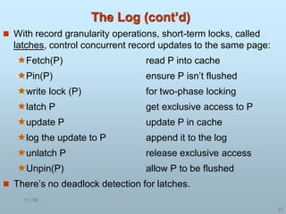
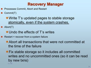
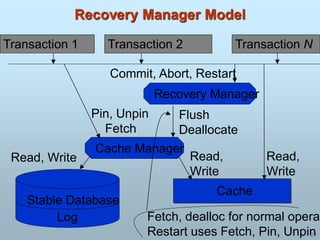
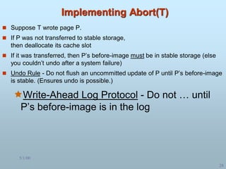
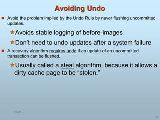
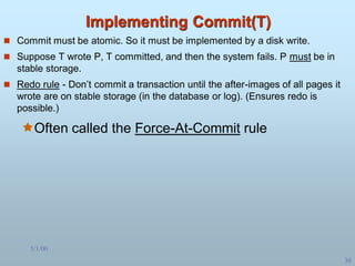
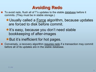
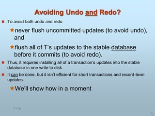
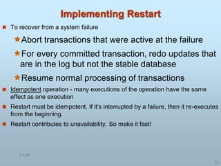
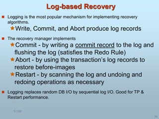
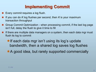
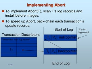
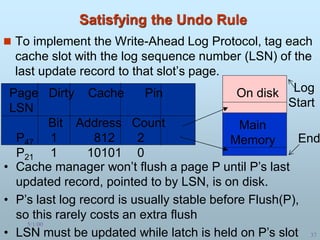
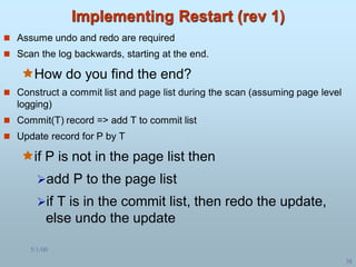
![5/1/00
40
Checkpoints
Problem - Prevent Restart from scanning back to the start of the log
A checkpoint is a procedure to limit the amount of work for Restart
Commit-consistent checkpointing
Stop accepting new update, commit, and abort
operations
make list of [active transaction, pointer to last log
record]
flush all dirty pages
append a checkpoint record to log, which includes
the list
resume normal processing
Database and log are now mutually consistent](https://image.slidesharecdn.com/dbmscombine-251224035216-cbcde31f/85/dbms-combine-with-sql-for-engineering-pdf-763-320.jpg)
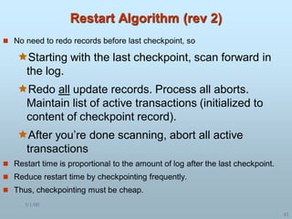
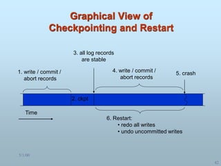
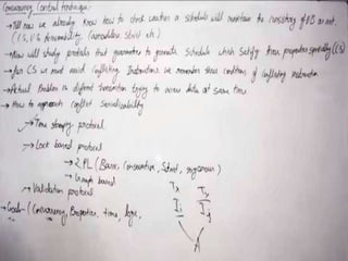
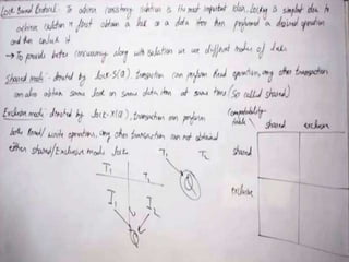
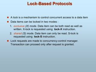
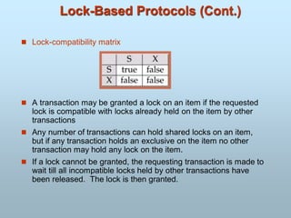
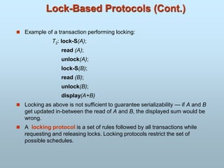
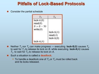
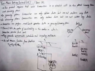
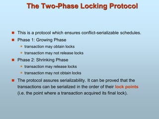
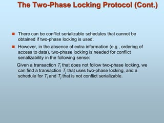
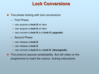
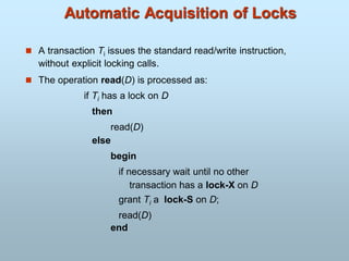
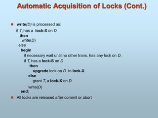
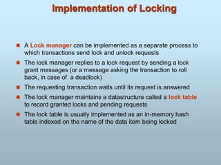
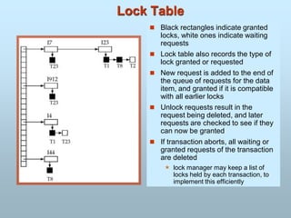
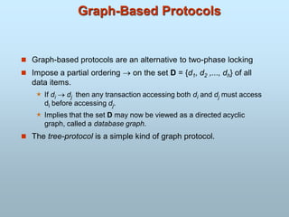
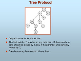

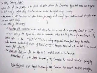
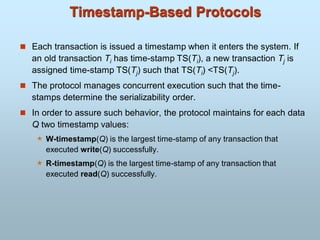
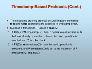
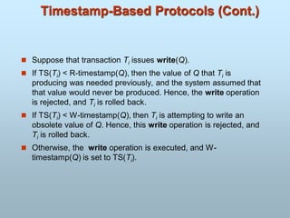
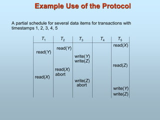
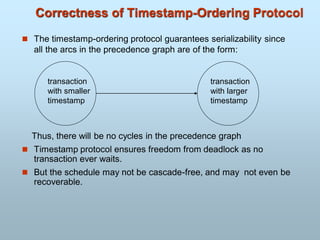
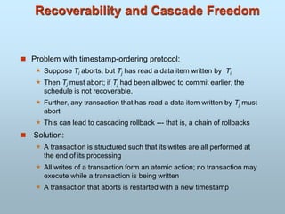
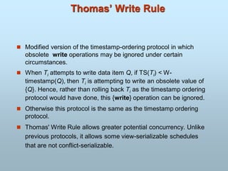
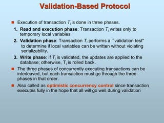
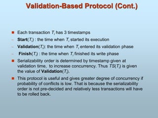
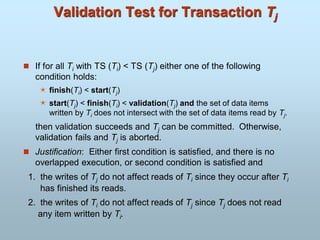
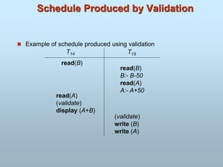
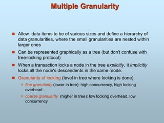
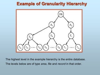
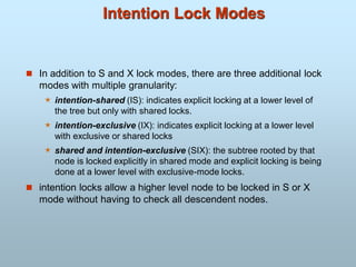
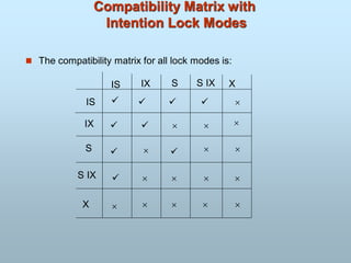
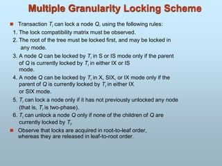
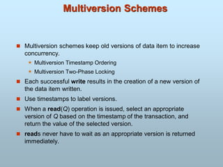
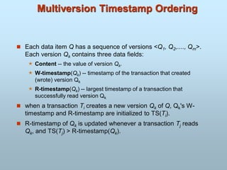
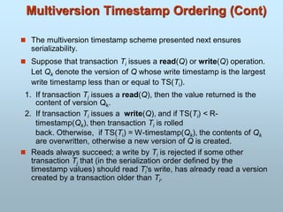
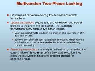
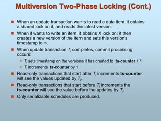
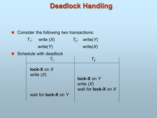
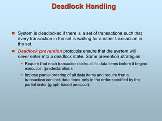
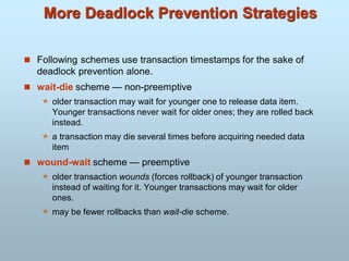

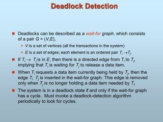
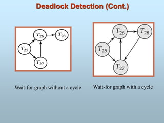
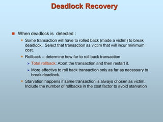
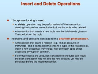
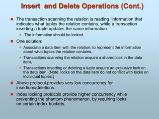
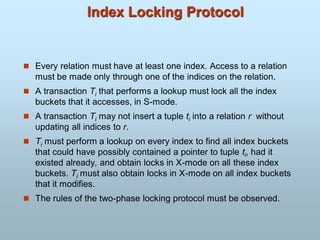
![Weak Levels of Consistency
Degree-two consistency: differs from two-phase locking in that
S-locks may be released at any time, and locks may be acquired
at any time
X-locks must be held till end of transaction
Serializability is not guaranteed, programmer must ensure that no
erroneous database state will occur]
Cursor stability:
For reads, each tuple is locked, read, and lock is immediately
released
X-locks are held till end of transaction
Special case of degree-two consistency](https://image.slidesharecdn.com/dbmscombine-251224035216-cbcde31f/85/dbms-combine-with-sql-for-engineering-pdf-818-320.jpg)