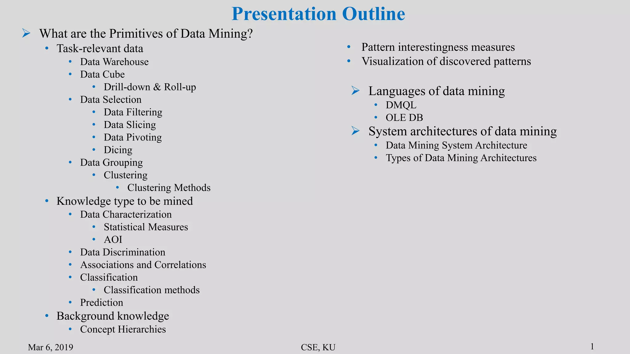
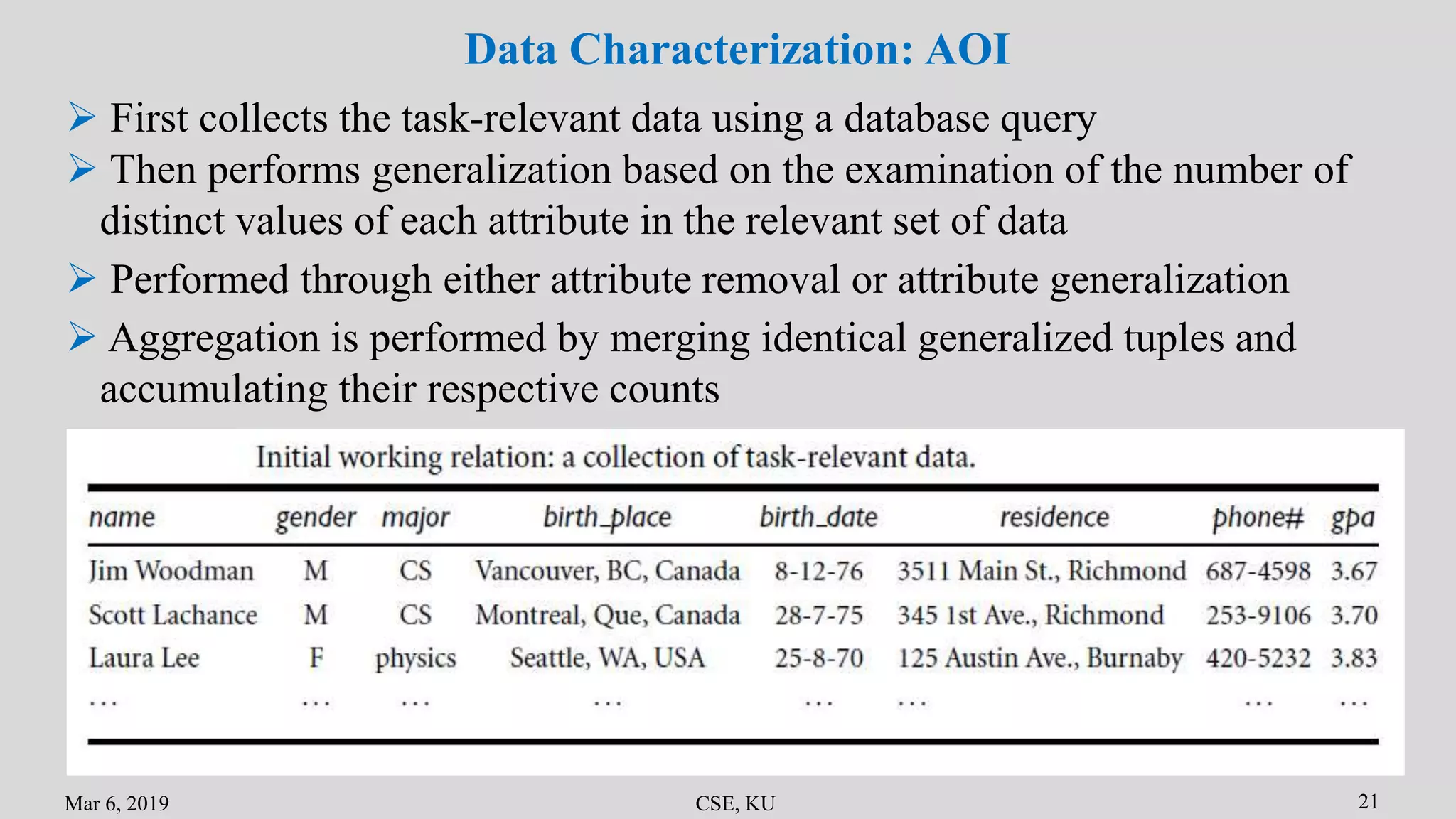
Science 7 - LAND and SEA BREEZE and its Characteristics
Data Mining Primitives, Languages & Systems
1. Advanced Data Mining
Lec-4: Data Mining Primitives, Languages & Systems
[Class Presentation]
Presented by
Niloy Sikder
ID: MSc 190221
CSE Discipline
Khulna University, Khulna
2. Mar 6, 2019 CSE, KU 1
Presentation Outline
What are the Primitives of Data Mining?
• Task-relevant data
• Data Warehouse
• Data Cube
• Drill-down & Roll-up
• Data Selection
• Data Filtering
• Data Slicing
• Data Pivoting
• Dicing
• Data Grouping
• Clustering
• Clustering Methods
• Knowledge type to be mined
• Data Characterization
• Statistical Measures
• AOI
• Data Discrimination
• Associations and Correlations
• Classification
• Classification methods
• Prediction
• Background knowledge
• Concept Hierarchies
System architectures of data mining
• Data Mining System Architecture
• Types of Data Mining Architectures
Languages of data mining
• DMQL
• OLE DB
• Pattern interestingness measures
• Visualization of discovered patterns
4. Mar 6, 2019 CSE, KU 3
What are the Primitives of Data Mining?
The set of task-relevant data to be mined
The kind of knowledge to be mined
The background knowledge
Interestingness measures and thresholds for pattern evaluation
The expected representation for visualizing the discovered patterns
5. Mar 6, 2019 CSE, KU 4
The First Primitive of Data Mining: Task-relevant Data
Portions of the database or the set of data in which the user is interested.
Fig. 1: Task-relevant data for specifying a data mining task
6. Mar 6, 2019 CSE, KU 5
Task-relevant Data: Data Warehouse
A Warehouse is a repository of information usually from multiple sources
Fig. 2: Typical framework of a data warehouse for AllElectronics.
Usually resides at a single site
Constructed via a process of data cleaning, data integration, data
transformation, data loading, and periodic data refreshing
7. Mar 6, 2019 CSE, KU 6
Task-relevant Data: Data Cube
A multidimensional data structure inside a data warehouse
Fig. 3: Summarized data for AllElectronics.
Each dimension corresponds to an attribute
Each cell stores the value of some aggregate measure
8. Mar 6, 2019 CSE, KU 7
Data Cube: Drill-down & Roll-up
A presentation of data at different levels of abstraction
Fig. 3: Summarized data resulting drill-down and roll-up operations on the cube.
Allow the user to view the data at differing degrees of summarization
9. Mar 6, 2019 CSE, KU 8
Task-relevant Data: Data Selection
The process of retrieving relevant data to the analysis task from database
Data can be specified by condition-based data filtering, slicing, pivoting or
dicing a data cube
Data Selection: Data Filtering
Selective presentation or deliberate manipulation of information to make it
more acceptable or favorable to the mining model
Reduces the content of noise or errors from raw data
DSP – Low-pass, High-pass, Band-pass, Notch, Comb, Cut-off frequency
DIP – Convolution, Gaussian, Bilateral, adaptive, Coye
Database – Various SQL filters
10. Mar 6, 2019 CSE, KU 9
Data Selection: Data Filtering (cont.)
Grafil (Graph Similarity Filtering), was developed to filter graphs
efficiently in large-scale graph databases
11. Mar 6, 2019 CSE, KU 10
Data Selection: Data Slicing
Selecting a group of cells from the entire multidimensional array by
specifying a specific value for one or more dimensions
12. Mar 6, 2019 CSE, KU 11
Data Selection: Data Pivoting
Aggregating over all dimensions except two
Results in a two-dimensional cross tabulation reducing a dimension
13. Mar 6, 2019 CSE, KU 12
Data Selection: Dicing
Selecting a subset of cells by specifying a range of attribute values
Equivalent to defining a sub-array from the complete array
14. Mar 6, 2019 CSE, KU 13
Curse of Dimensionality
Dimensionality of a data set is the number of attributes that the objects in
the data set possess
Difficult to analyze and visualize high-dimensional data
Data becomes increasingly sparse in the space that it occupies
Clustering high-dimensional data is challenging
All the dimensions may not be relevant
Increases computational complexity
Requires more processing power & time
15. Mar 6, 2019 CSE, KU 14
Task-relevant Data: Data Grouping
Clustering is the process of grouping the data into classes or clusters
Objects within a cluster have high similarity in comparison to one another
but are very dissimilar to objects in other clusters
Can also be used for outlier detection
16. Mar 6, 2019 CSE, KU 15
Data Grouping: Clustering
Typical requirements of clustering in data mining:
Scalability
Ability to deal with different types of attributes/ data types
Discovery of clusters with arbitrary shape
Minimal requirements for domain knowledge to determine input parameters
Ability to deal with noisy data
Incremental clustering and insensitivity to the order of input records
High dimensionality
Constraint-based clustering
Interpretability and usability
17. Mar 6, 2019 CSE, KU 16
Data Grouping: Clustering Methods
Partitioning methods:
k-Means Method
k-Medoids Method
CLARANS (for large databases)
Hierarchical methods:
Agglomerative and Divisive
Hierarchical Clustering
BIRCH
ROCK
Chameleon
Density-based methods:
DBSCAN
OPTICS
DENCLUE
Grid-based methods:
STING
WaveCluster
19. Mar 6, 2019 CSE, KU 18
The Second Primitive of Data Mining: Knowledge Types
Important to specify the kind of knowledge to be mined, as this determines
the data mining function to be performed
Fig. 1: Task-relevant data for specifying a data mining task
User can be more specific and provide pattern templates (metarules or
metaqueries) that all discovered patterns must match
20. Mar 6, 2019 CSE, KU 19
Knowledge Types: Data Characterization
A summary of the general characteristics or features of a target class of data
Summarizes data by replacing relatively low-level values (numeric) with
higher-level concepts (young, middle-aged, and senior)
Several methods for effective data characterization:
Statistical measures
Attribute-oriented induction (AOI)
Output can be presented in pie charts, bar charts, curves, multidimensional
data cubes, and multidimensional tables
21. Mar 6, 2019 CSE, KU 20
Data Characterization: Statistical Measures
Central tendency of data – mean, weighted mean, median, mode
Dispersion of data – range, quartiles, variance, standard deviation
Graphical representations – histograms, boxplots, quantile plots, quantile
plots, scatter plots, scatter-plot matrices
22. Mar 6, 2019 CSE, KU 21
Data Characterization: AOI
First collects the task-relevant data using a database query
Then performs generalization based on the examination of the number of
distinct values of each attribute in the relevant set of data
Performed through either attribute removal or attribute generalization
Aggregation is performed by merging identical generalized tuples and
accumulating their respective counts
23. Mar 6, 2019 CSE, KU 22
Knowledge Types: Data Discrimination
A comparison of the general features of target class data objects with a set
of contrasting classes
The target and contrasting classes can be specified by the user
They must be comparable i.e. share similar dimensions and attributes
Data discrimination procedure:
Data collection: query processing
Dimension relevance analysis: select only the highly relevant dimensions for
further analysis
Synchronous generalization: results in a prime target class relation
Presentation of the derived comparison: tables, graphs, and rules
24. Mar 6, 2019 CSE, KU 23
Knowledge Types: Data Discrimination (cont.)
Compare the general properties between the graduate and undergraduate students at
BigUniversity, given the attributes name, gender, major, birth place, birth date, residence,
phone#, and gpa. This data mining task can be expressed in DMQL as follows:
Example:
use Big University_DB
mine comparison as “grad vs undergrad_students”
in relevance to name, gender, major, birth_place, birth_date, residence, phone#, gpa
for “graduate_students”
where status in “graduate”
versus “undergraduate_students”
where status in “undergraduate”
analyze count%
from student
25. Mar 6, 2019 CSE, KU 24
Knowledge Types: Associations and Correlations
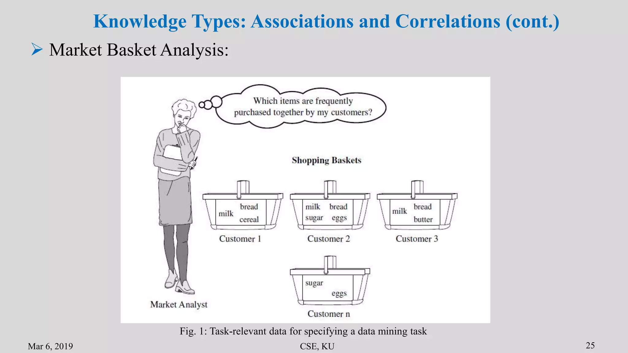
Frequent patterns, are the patterns that occur frequently in data
buys(X; “computer”)) => buys(X; “software”) [support = 1%; confidence = 50%]
Mining frequent patterns leads to the discovery of interesting associations
and correlations within data
A frequent itemset refers to a set of items that frequently appear together in
a transactional data set
age(X, “20:::29”) ^ income(X, “20K:::29K”)) => buys(X, “CD player”) [support = 2%,
confidence = 60%]
26. Mar 6, 2019 CSE, KU 25
Market Basket Analysis:
Fig. 1: Task-relevant data for specifying a data mining task
Knowledge Types: Associations and Correlations (cont.)
27. Mar 6, 2019 CSE, KU 26
Knowledge Types: Classification
The process of finding a model (or function) that describes and
distinguishes data classes or concepts
28. Mar 6, 2019 CSE, KU 27
Knowledge Types: Classification (cont.)
29. Mar 6, 2019 CSE, KU 28
Classification by Decision Tree Induction
ID3, C4,5, CART
Bayesian Classification
Knowledge Types: Classification methods
Rule-Based Classification
Classification by Back-propagation
Support Vector Machines
Lazy Learners (or Learning from Your Neighbors)
Genetic Algorithms
Ensemble Methods: Bagging & Boosting
Fuzzy Set Approaches
Rough Set Approach
30. Mar 6, 2019 CSE, KU 29
Linear Regression
Nonlinear Regression
Knowledge Types: Prediction Methods
Log-linear models
Decision tree induction
Ensemble Methods: Bagging & Boosting
Forcasting
The process of finding a value/ range of an attribute for a given condition
from the training dataset
31. Mar 6, 2019 CSE, KU 30
The Third Primitive of Data Mining: Background Knowledge
Useful to guide the knowledge discovery process and evaluate patterns
32. Mar 6, 2019 CSE, KU 31
Defines a sequence of mappings from a set of low-level concepts to higher-
level, more general concepts
Allows data to be mined at multiple levels of abstraction
Background Knowledge: Concept Hierarchies
33. Mar 6, 2019 CSE, KU 32
Interestingness Measures and Thresholds for Pattern Evaluation
May be used to guide the mining process or, after discovery, to evaluate the
discovered patterns
Different kinds of knowledge may have different interestingness measures
34. Mar 6, 2019 CSE, KU 33
Visualization of Discovered Patterns
Discovered knowledge should be expressed in high-level languages, visual
representations, or other expressive forms
Knowledge should be easily understood and directly usable by humans
especially crucial if the data mining system is to be interactive
36. Mar 6, 2019 CSE, KU 35
Data Mining Language: DMQL
DMQL (Data Mining Query Language):
Based on & similar to the Structured Query Language (SQL)
Can work with databases and data warehouses as well
Can easily be integrated with the relational query language
Example:
use database AllElectronics_db
use hierarchy location_hierarchy for T.branch, age_hierarchy for C.age
mine classification as promising_customers
in relevance to C.age, C.income, I.type, I.place_made, T.branch
from customer C, item I, transaction T
where I.item_ID = T.item_ID and C.cust_ID = T.cust_ID
and C.income >= 40,000 and I.price >= 100
group by T.cust_ID
having sum(I.price) >= 1,000
display as rules
37. Mar 6, 2019 CSE, KU 36
Data Mining Language: OLE DB
Microsoft’s OLE DB (Object Linking and Embedding, Database):
A major step toward the standardization of data mining language primitives
and aims to become the industry standard
Adopts many concepts in relational database systems and applies them to the
data mining field, providing a standard programming API.
Designed to allow data mining client applications (or data mining consumers)
to consume data mining services from various data mining softwares.
Has DMX (Data Mining eXtensions) at the core, which is SQL-like
OLE DB for DM describes an abstraction of the data mining process:
Model creation
Model training
Model prediction and browsing
38. Mar 6, 2019 CSE, KU 37
Data Mining Language: OLE DB (cont.)
39. Mar 6, 2019 CSE, KU 38
Data Mining Language: OLE DB (cont.)
Example:
create mining model prediction
( customer_ID long key,
gender text discrete,
age long discretized(),
income long continuous,
profession text discrete,
)
using Microsoft_Decision_Trees
41. Mar 6, 2019 CSE, KU 40
Data Mining System Architecture
42. Mar 6, 2019 CSE, KU 41
Types of Data Mining Architectures
No-coupling Data Mining:
Data mining system does not use any functionality of a database or warehouse
Retrieves data from a particular data sources
Does not take any advantages of a database
Considered a poor architecture but used for simple data mining applications
Loose Coupling Data Mining:
System may use some of the functions of database and data warehouse system
Fetches the data from the data respiratory managed by the system
Stores the mining result either in a file or in a designated place in a database or
in a data warehouse
Does not provide high scalability and high performance.
43. Mar 6, 2019 CSE, KU 42
Types of Data Mining Architectures (cont.)
Semi-Tight Coupling Data Mining:
Mining system is linked with a database or a data warehouse system
Uses several features of data warehouse systems
Applications include sorting, indexing & aggregation
Efficient implementations of a few data mining primitives can be provided
Tight Coupling Data Mining:
Mining system is fully integrated into a database or data warehouse system
Mining subsystem is treated as one functional component of an IR system
Provides system scalability, high performance, and integrated information
45. References
[1] Data Mining: Concepts and Techniques Second Edition - Jiawei Han, Micheline Kamber
[2] Introduction to Data Mining - Tan Steinbach Kumar
[3] https://data-flair.training/blogs/data-mining-architecture/
[4] https://www.tutorialspoint.com/data_mining/dm_systems.htm
Editor's Notes
Reference [1]: (Concepts and Techniques Second Edition - Jiawei Han, Micheline Kamber)
Section 1.7, page: 31
Ref [1], p. 31,32
Ref [1], Sec 1.3.2, p. 12
Suppose that AllElectronics is a successful international company, with branches around
the world. Each branch has its own set of databases. The president of AllElectronics has
asked you to provide an analysis of the company’s sales per item type per branch for the
third quarter. This is a difficult task, particularly since the relevant data are spread out
over several databases, physically located at numerous sites.
If AllElectronics had a data warehouse, this task would be easy. A data warehouse
is a repository of information collected from multiple sources, stored under
a unified schema, and that usually resides at a single site. Data warehouses are constructed
via a process of data cleaning, data integration, data transformation, data
loading, and periodic data refreshing. This process is discussed in Chapters 2 and 3.
Figure 1.7 shows the typical framework for construction and use of a data warehouse
for AllElectronics.
Ref [1], Example 1.2, p. 13
A data cube for AllElectronics. A data cube for summarized sales data of AllElectronics
is presented in Figure 1.8(a). The cube has three dimensions: address (with city values
Chicago, New York, Toronto, Vancouver), time (with quarter values Q1, Q2, Q3, Q4), and
item(with itemtype values home entertainment, computer, phone, security). The aggregate
value stored in each cell of the cube is sales amount (in thousands). For example, the total
sales forthefirstquarter,Q1, for itemsrelatingtosecuritysystemsinVancouver is$400,000,
as stored in cell hVancouver, Q1, securityi.Additional cubesmay be used to store aggregate
sumsover eachdimension, corresponding to the aggregate values obtained using different
SQL group-bys (e.g., the total sales amount per city and quarter, or per city and item, or
per quarter and item, or per each individual dimension).
Ref [1], Example 1.2, p. 13
Ref [1], Example 9.6, p. 554
Ref [2], Section 3.4.1 , p. 131-133
Ref [2], Section 3.4.3 , p. 137
Table 3.12 shows the result of summing over all locations for various combinations of date and product. For simplicity, assume that all the dates are within one year. If there are 365 days in a year and 1000 products, then Table 3.12 has 365,000 entries (totals), one for each product-data pair. We couldalso specify the store location and date and sum over products, or specify thelocation and product and sum over all dates
Ref [2], p. 138
Ref [2], Section 2.1.2 , p. 29
Ref [1], Section 7.1 , p. 383
Clustering - data segmentation
Ref [1], Section 7.1 , p. 385
Many clustering algorithms determine clusters based on Euclidean or Manhattan distance measures which tend to find spherical clusters with similar size and density.
Clustering - data segmentation
Many clustering algorithms determine clusters based on Euclidean or Manhattan distance measures which tend to find spherical clusters with similar size and density.
CLARANS Clustering LARge Applications
BIRCH: Balanced Iterative Reducing and Clustering Using Hierarchies
ROCK (RObust Clustering using linKs)
DBSCAN Density-Based Spatial Clustering of Applications with Noise
OPTICS Ordering Points to Identify the Clustering Structure
DENCLUE DENsity-based CLUstEring
STING: STatistical INformation Grid
Ref [1], Section 4.3.1 , p. 199
Attribute-oriented induction. Here we show how attribute-oriented induction is performed on the initial working relation of Table 4.12. For each attribute of the relation,the generalization proceeds as follows:1. name: Since there are a large number of distinct values for name and there is nogeneralization operation defined on it, this attribute is removed.2. gender: Since there are only two distinct values for gender, this attribute is retainedand no generalization is performed on it.3. major: Suppose that a concept hierarchy has been defined that allows the attributemajor to be generalized to the values farts&science, engineering, businessg. Supposealso that the attribute generalization threshold is set to 5, and that there are more than20 distinct values for major in the initial working relation. By attribute generalizationand attribute generalization control, major is therefore generalized by climbing thegiven concept hierarchy.4. birth place: This attribute has a large number of distinct values; therefore, we wouldlike to generalize it. Suppose that a concept hierarchy exists for birth place, defined as “city < province or state < country”. If the number of distinct values for countryin the initial working relation is greater than the attribute generalization threshold,then birth place should be removed, because even though a generalization operatorexists for it, the generalization threshold would not be satisfied. If instead, the numberof distinct values for country is less than the attribute generalization threshold, thenbirth place should be generalized to birth country.5. birth date: Suppose that a hierarchy exists that can generalize birth date to age, and ageto age range, and that the number of age ranges (or intervals) is small with respect tothe attribute generalization threshold. Generalization of birth date should thereforetake place.6. residence:Supposethatresidenceisdefinedbytheattributesnumber,street,residence city,residence province or state, and residence country. The number of distinct values fornumber and street will likely be very high, since these concepts are quite low level. Theattributes number and street should therefore be removed, so that residence is thengeneralized to residence city, which contains fewer distinct values.7. phone#: As with the attribute name above, this attribute contains too many distinctvalues and should therefore be removed in generalization.8. gpa: Suppose that a concept hierarchy exists for gpa that groups values for gradepoint average into numerical intervals like f3.75–4.0, 3.5–3.75,...g, which in turnare grouped into descriptive values, such as fexcellent, very good,...g. The attributecan therefore be generalized.
Ref [1], Example 1.4 , p. 22
class comparison (also known as discrimination)
Ref [1], Example 4.27 , p. 212
Ref [1], Example 5.1.2 , p. 230
Ref [1], Example 5.1.1 , p. 228
Ref [1], Example 6.1, p. 287
Ref [1], p. 31,32
Ref [1], Section 3.2.5, p. 121
Ref [1], p. 31,32
A data mining system can uncover thousands of patterns. Many of the patterns discovered may be uninteresting to the given user, either because they represent common knowledge or lack novelty. Several challenges remain regarding the development of techniques to assess the interestingness of discovered patterns, particularly with regard to subjective measures that estimate the value of patterns with respect to a given user class, based on user beliefs or expectations. The use of interestingness measures or user-specified constraints to guide the discovery process and reduce the search space is another active area of research.
Ref [1], p. 31, 32
Mining classification rules. Suppose, as a marketing manager of AllElectronics, you would like to classify customers based on their buying patterns. You are especially interested in those customers whose salary is no less than $40,000, and who have bought more than $1,000 worth of items, each of which is priced at no less than $100. In particular, you are interested in the customer’s age, income, the types of items purchased, the purchase location, and where the items were made. You would like to view the resulting classification in the form of rules.