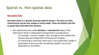
GIS Data
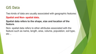
Two kindsof data are usually associated with geographic features:
Spatial and Non- spatial data.
Spatial data refers to the shape, size and location of the
feature.
Non- spatial data refers to other attributes associated with the
feature such as name, length, area, volume, population, soil type,
etc ..
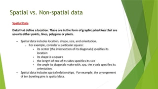
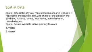
Spatial Data
Spatial datais the physical representation of earth features. It
represents the location, size, and shape of the object in the
earth i.e., building, ponds, mountains, administration,
boundaries, etc.
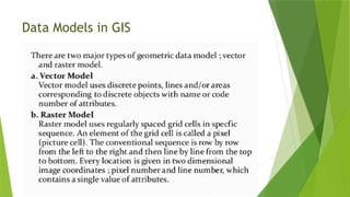
Spatial Data is available in two primary formats
1. Vector
2. Raster
5.
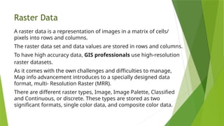
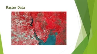
Raster Data
A rasterdata is a representation of images in a matrix of cells/
pixels into rows and columns.
The raster data set and data values are stored in rows and columns.
To have high accuracy data, GIS professionals use high-resolution
raster datasets.
As it comes with the own challenges and difficulties to manage,
Map info advancement introduces to a specially designed data
format, multi- Resolution Raster (MRR).
There are different raster types, Image, Image Palette, Classified
and Continuous, or discrete. These types are stored as two
significant formats, single color data, and composite color data.
Raster File Formats
Portable Network Graphics (PNG)
Joint Photographic Experts Group (JPEG2000)
JPEG File Interchange Format (JFIF)
Multi-resolution Seamless Image Database (MrSID)
Network Common Data Form (netCDF)
Digital raster graphic(DRG)
ARC Digitized Raster Graphic (ADRG)
Enhanced Compressed ARC Raster Graphics (ECRG)
Compressed ARC Digitized Raster Graphics (CADRG)
8.
Raster File Formats
Raster Product Format (RPF)
Binary file – Band Interleaved by Pixel (BIP), Band Interleaved by
Line (BIL), Band Sequential (BSQ)
Enhanced Compressed Wavelet (ECW)
Extensible N-Dimensional Data Format (NDF)
GDAL Virtual Format (VRT)
Tagged Image File Formats (TIFF)
Geo Tagged Image File Formats (GeoTIFF)
Graphic Interchange Format (GIF)
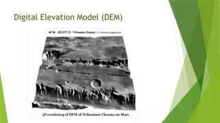
Digital Elevation Model (DEM)
9.
Raster File Formats
RS Landsat
ArcInfo Grid
Airborne Synthetic Aperture Radar (AIRSAR) Polarimetric
Bitmap (BMP), device-independent bitmap (DIB) format, or
Microsoft Windows bitmap
BSB
Controlled Image Base (CIB)
Digital Geographic Information Exchange Standard (DIGEST)
File geodatabase
ENVI Header
10.
Raster File Formats
Golden Software Grid (.grd)
GRIB
Hierarchical Data Format (HDF) 4
HGT
High-Resolution Elevation (HRE)
Integrated Software for Imagers and Spectrometers (ISIS)
Shuttle Radar Topography Mission (SRTM)
Terragen terrain
11.
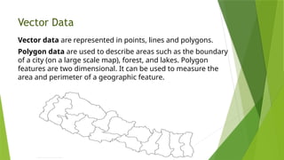
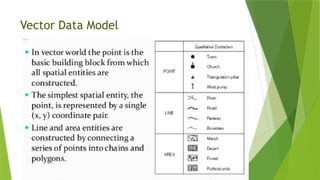
Vector Data
Vector dataare represented in points, lines and polygons.
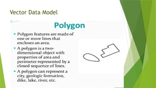
Polygon data are used to describe areas such as the boundary
of a city (on a large scale map), forest, and lakes. Polygon
features are two dimensional. It can be used to measure the
area and perimeter of a geographic feature.
12.
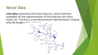
Vector Data
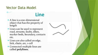
Line datarepresents the linear features. Some Common
examples for the representation of line features are rivers,
roads, etc. The line is a one-dimensional representation. It gives
only the length of the element.
13.
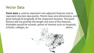
Vector Data
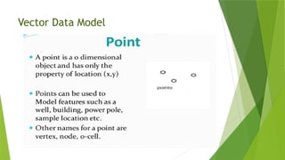
Point datais used to represent non-adjacent features and to
represent discrete data points. Points have zero dimensions, and it
gives latitude & longitude of the respective location. The point
feature will not provide the length and area of the features.
Examples would be schools, points of interest such as hospitals,
schools, colleges, worship centers, and more other locations.
Vector File Formats
Vector Product Format (VPF)
Esri TIN
Geography Markup Language (GML)
SpatiaLite
OSM (OpenStreetMap)
Scalable Vector Graphics
National Transfer Format (NTF)
SOSI
MapInfo TAB format
16.
Vector File Formats
GPS exchange Format (GPX)
IDRISI Vector
Geographic Base File-Dual Independent Mask Encoding (GBF-
DIME)
Delimited Text Files
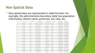
Non-Spatial Data
Non-spatialdata are represented in table formats. For
example, the administrative boundary table has population
information, district name, provinces, sex ratio, etc.
Functions of GIS
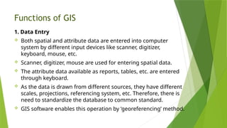
1.Data Entry
Both spatial and attribute data are entered into computer
system by different input devices like scanner, digitizer,
keyboard, mouse, etc.
Scanner, digitizer, mouse are used for entering spatial data.
The attribute data available as reports, tables, etc. are entered
through keyboard.
As the data is drawn from different sources, they have different
scales, projections, referencing system, etc. Therefore, there is
need to standardize the database to common standard.
GIS software enables this operation by ‘georeferencing’ method.
45.
Functions of GIS
2.Storing of data
The different spatial entities which represent different
features of real world can be stored in two different formats
in the computer – Raster format & Vector format
The knowledge of these formats in which spatial data are
stored, is required for decision makers as it affects the
accuracy of the data, their analysis, storing capacity of
computer, etc.
46.
Functions of GIS
3.Data Analysis (Map Analysis)
Different types of spatial data analysis can be performed by GIS,
performing queries, network analysis, overlay analysis, model
building, etc.
Since GIS stores both spatial and non-spatial data and links them
together, it can perform different types of queries.
For example, by joining the spatial data and its attributes and then by
performing queries, one can see on map, the water of which tube
wells having chlorine content more than 200 mg/liter.
Similarly, one can see on map, the roads constructed before 1980
which needs to be repaired.
In the same way, which area of a given forest having more than 60%
tree density on Map.
47.
Functions of GIS
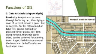
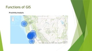
3.Data Analysis (Map Analysis)
Proximity Analysis can be done
through buffering i.e., identifying a
zone of interest around a point, line
or polygon. For Ex, 10m around on
tube well can be marked for
planting flower plants, (or) 50m
along National Highways (both
sides) can be buffered for planting
trees. A specified distance around
the forest can be buffered as no
habitation zone.
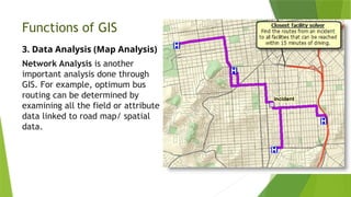
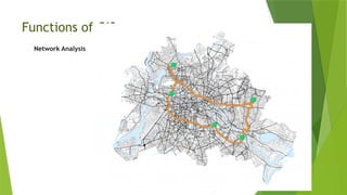
Functions of GIS
3.Data Analysis (Map Analysis)
Network Analysis is another
important analysis done through
GIS. For example, optimum bus
routing can be determined by
examining all the field or attribute
data linked to road map/ spatial
data.
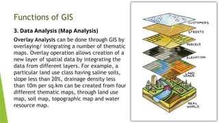
Functions of GIS
3.Data Analysis (Map Analysis)
Overlay Analysis can be done through GIS by
overlaying/ integrating a number of thematic
maps. Overlay operation allows creation of a
new layer of spatial data by integrating the
data from different layers. For example, a
particular land use class having saline soils,
slope less than 20%, drainage density less
than 10m per sq.km can be created from four
different thematic maps, through land use
map, soil map, topographic map and water
resource map.
52.
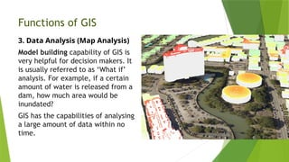
Functions of GIS
3.Data Analysis (Map Analysis)
Model building capability of GIS is
very helpful for decision makers. It
is usually referred to as ‘What if’
analysis. For example, if a certain
amount of water is released from a
dam, how much area would be
inundated?
GIS has the capabilities of analysing
a large amount of data within no
time.
53.
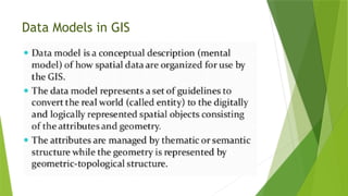
Data Models
A datamodel is a description or view of the real world.
Data modeling is a process that formalizes the description or
view at different levels of data abstraction.
Since, the real world is made up of complex spatial objects
and phenomena, it is practically impossible for a single data
model to represent everything that is present.
This means that different users may have different data
models when they attempt to collect data in the same
location.
54.
Data Models
1. Conceptualmodels
The different views of the same urban area obtained by the
engineer, the developer and the geographer are called
conceptual models.
It represents the user’s perception of the real world. Here, data
abstraction is strictly limited to the description of the
information contents of the user’s view of the real world,
without any concern for computer implementation.
55.
Data Models
2. Logicaldata models
It represents an implementation – oriented view of the
database.
It represents the real world by means of diagrams, lists and
tables designed to reflect the recording of data in terms of some
formal language.
It is software dependent.
There are three classic logical data models.
The relational data model
The network data model
The hierarchical data model
56.
Data Models
3. Physicaldata models
It represents the hardware implementation – oriented view of
the database.
It is the 3rd
level of data abstraction.
It describes the physical storage (or file format) of the data in
the computer by record format, record ordering and access
paths.
It is hardware dependent.
It is intended for system programmer and database
administrator, and not for general end users.
57.
Data Models
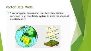
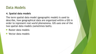
4. Spatialdata models
The term spatial data model (geographic model) is used to
describe, how geographical data are organized within a GIS in
order to represent real world phenomena. GIS uses one of the
two spatial data models (sometimes both).
Raster data models
Vector data models
58.
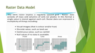
Data Models
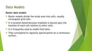
Raster datamodels
Raster models divide the study area into cells, usually
rectangular grid cells.
It is location based because emphasis is placed upon the
location of each cell relative to other cells.
It is frequently used to model field data.
They correspond to regularly spaced points on a continuous
surface.
59.
Data Models
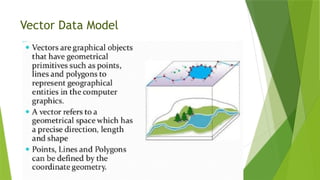
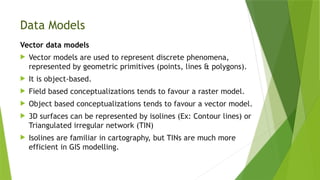
Vector datamodels
Vector models are used to represent discrete phenomena,
represented by geometric primitives (points, lines & polygons).
It is object-based.
Field based conceptualizations tends to favour a raster model.
Object based conceptualizations tends to favour a vector model.
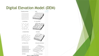
3D surfaces can be represented by isolines (Ex: Contour lines) or
Triangulated irregular network (TIN)
Isolines are familiar in cartography, but TINs are much more
efficient in GIS modelling.
60.
Database Models
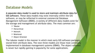
A separatedata model is used to store and maintain attribute data for
GIS software. These data models may exist internally within the GIS
software, or may be reflected in external commercial Database
Management Software (DBMS). A variety of different data models exist for
the storage and management of attribute data. The most common are:
Tabular
Hierarchical
Network
Relational
Object Oriented
The tabular model is the manner in which most early GIS software packages
stored their attribute data. The next three models are those most commonly
implemented in database management systems (DBMS). The object oriented
is newer but rapidly gaining in popularity for some applications.
61.
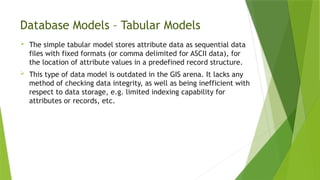
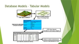
Database Models –Tabular Models
The simple tabular model stores attribute data as sequential data
files with fixed formats (or comma delimited for ASCII data), for
the location of attribute values in a predefined record structure.
This type of data model is outdated in the GIS arena. It lacks any
method of checking data integrity, as well as being inefficient with
respect to data storage, e.g. limited indexing capability for
attributes or records, etc.
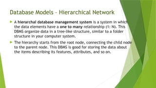
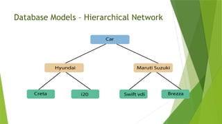
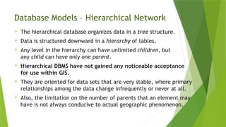
Database Models –Hierarchical Network
A hierarchal database management system is a system in which
the data elements have a one to many relationship (1: N). This
DBMS organize data in a tree-like structure, similar to a folder
structure in your computer system.
The hierarchy starts from the root node, connecting the child node
to the parent node. This DBMS is good for storing the data about
the items describing its features, attributes, and so on.
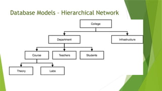
Database Models –Hierarchical Network
The hierarchical database organizes data in a tree structure.
Data is structured downward in a hierarchy of tables.
Any level in the hierarchy can have unlimited children, but
any child can have only one parent.
Hierarchical DBMS have not gained any noticeable acceptance
for use within GIS.
They are oriented for data sets that are very stable, where primary
relationships among the data change infrequently or never at all.
Also, the limitation on the number of parents that an element may
have is not always conducive to actual geographic phenomenon.
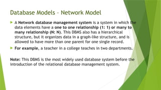
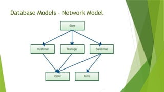
Database Models –Network Model
A Network database management system is a system in which the
data elements have a one to one relationship (1: 1) or many to
many relationship (N: N). This DBMS also has a hierarchical
structure, but it organizes data in a graph-like structure, and is
allowed to have more than one parent for one single record.
For example, a teacher in a college teaches in two departments.
Note: This DBMS is the most widely used database system before the
introduction of the relational database management system.
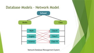
Database Models –Network Model
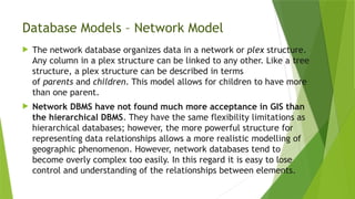
The network database organizes data in a network or plex structure.
Any column in a plex structure can be linked to any other. Like a tree
structure, a plex structure can be described in terms
of parents and children. This model allows for children to have more
than one parent.
Network DBMS have not found much more acceptance in GIS than
the hierarchical DBMS. They have the same flexibility limitations as
hierarchical databases; however, the more powerful structure for
representing data relationships allows a more realistic modelling of
geographic phenomenon. However, network databases tend to
become overly complex too easily. In this regard it is easy to lose
control and understanding of the relationships between elements.
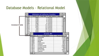
Database Models –Relational Model
A relational database management system (RDBMS) is a system in
which the data is organized in the two-dimensional tables using rows
and columns. This database management system was introduced
by E.F Codd in 1970.
It is called a ‘relational’ database because data within each table is
related to each other. Also, tables may be related to other tables in
the database by using certain concepts of keys. Each table in a
database has a key field that uniquely identifies each record. This
system is the most widely used DBMS. Relational database
management system software is available for large mainframe
systems as well as workstations and personal computers.
For example, Oracle Database, MySQL, Microsoft SQL Server, and IBM
DB2.
72.
Database Models –Relational Model
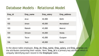
Emp_id Emp_name Emp_salary Emp_address
101 Arun 42,000 Delhi
102 Aman 40,000 Moradabad
103 Rakesh 43,000 Meerut
104 Shivam 44,000 Noida
105 Tarun 42,000 Gurgaon
106 Yash 40,000 Delhi
In the above table employee, Emp_id, Emp_name, Emp_salary, and Emp_address are
the attributes containing their values. Here, Emp_id is a primary key attribute which is
uniquely identifying each record in the Employee table.
73.
Database Models –Relational Model
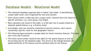
The relational database organizes data in tables. Each table, is identified by a
unique table name, and is organized by rows and columns.
Each column within a table also has a unique name. Columns store the values for a
specific attribute, e.g. cover group, tree height.
Rows represent one record in the table. In a GIS each row is usually linked to a
separate spatial feature, e.g. a forestry stand.
Accordingly, each row would be comprised of several columns, each column
containing a specific value for that geographic feature.
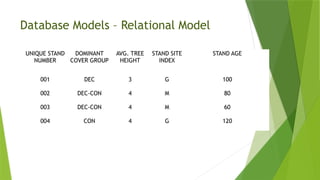
The following figure presents a sample table for forest inventory features. This table
has 4 rows and 5 columns.
The forest stand number would be the label for the spatial feature as well as
the primary key for the database table. This serves as the linkage between the
spatial definition of the feature and the attribute data for the feature.
74.
Database Models –Relational Model
UNIQUE STAND
NUMBER
DOMINANT
COVER GROUP
AVG. TREE
HEIGHT
STAND SITE
INDEX
STAND AGE
001 DEC 3 G 100
002 DEC-CON 4 M 80
003 DEC-CON 4 M 60
004 CON 4 G 120
75.
Database Models –Relational Model
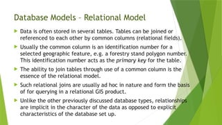
Data is often stored in several tables. Tables can be joined or
referenced to each other by common columns (relational fields).
Usually the common column is an identification number for a
selected geographic feature, e.g. a forestry stand polygon number.
This identification number acts as the primary key for the table.
The ability to join tables through use of a common column is the
essence of the relational model.
Such relational joins are usually ad hoc in nature and form the basis
of for querying in a relational GIS product.
Unlike the other previously discussed database types, relationships
are implicit in the character of the data as opposed to explicit
characteristics of the database set up.
76.
Database Models –Relational Model
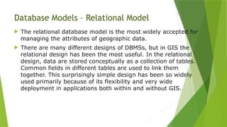
The relational database model is the most widely accepted for
managing the attributes of geographic data.
There are many different designs of DBMSs, but in GIS the
relational design has been the most useful. In the relational
design, data are stored conceptually as a collection of tables.
Common fields in different tables are used to link them
together. This surprisingly simple design has been so widely
used primarily because of its flexibility and very wide
deployment in applications both within and without GIS.
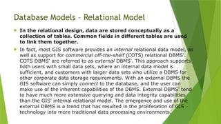
Database Models –Relational Model
In the relational design, data are stored conceptually as a
collection of tables. Common fields in different tables are used
to link them together.
In fact, most GIS software provides an internal relational data model, as
well as support for commercial off-the-shelf (COTS) relational DBMS'.
COTS DBMS' are referred to as external DBMS'. This approach supports
both users with small data sets, where an internal data model is
sufficient, and customers with larger data sets who utilize a DBMS for
other corporate data storage requirements. With an external DBMS the
GIS software can simply connect to the database, and the user can
make use of the inherent capabilities of the DBMS. External DBMS' tend
to have much more extensive querying and data integrity capabilities
than the GIS' internal relational model. The emergence and use of the
external DBMS is a trend that has resulted in the proliferation of GIS
technology into more traditional data processing environments.
79.
Database Models –Relational Model
The relational DBMS is attractive because of its:
simplicity in organization and data modelling.
flexibility - data can be manipulated in an ad hoc manner by
joining tables.
efficiency of storage - by the proper design of data tables
redundant data can be minimized; and
the non-procedural nature - queries on a relational database
do not need to take into account the internal organization of
the data.
The relational DBMS has emerged as the dominant commercial
data management tool in GIS implementation and application.
80.
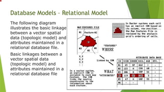
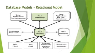
Database Models –Relational Model
The following diagram
illustrates the basic linkage
between a vector spatial
data (topologic model) and
attributes maintained in a
relational database file.
Basic linkages between a
vector spatial data
(topologic model) and
attributes maintained in a
relational database file
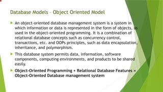
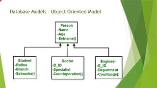
Database Models –Object Oriented Model
An object-oriented database management system is a system in
which information or data is represented in the form of objects, as
used in the object-oriented programming. It is a combination of
relational database concepts such as concurrency control,
transactions, etc. and OOPs principles, such as data encapsulation,
inheritance, and polymorphism.
This database system permits data, information, software
components, computing environments, and products to be shared
easily.
Object-Oriented Programming + Relational Database Features =
Object-Oriented Database management system
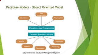
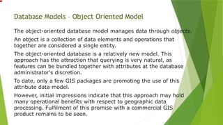
Database Models –Object Oriented Model
The object-oriented database model manages data through objects.
An object is a collection of data elements and operations that
together are considered a single entity.
The object-oriented database is a relatively new model. This
approach has the attraction that querying is very natural, as
features can be bundled together with attributes at the database
administrator's discretion.
To date, only a few GIS packages are promoting the use of this
attribute data model.
However, initial impressions indicate that this approach may hold
many operational benefits with respect to geographic data
processing. Fulfilment of this promise with a commercial GIS
product remains to be seen.
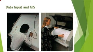
Data Input andGIS
Data input is the procedure of encoding data into a computer-
readable form and writing the data to the GIS data base. There
are two types of data to be entered in a GIS - spatial (geographic
location of features) and non-spatial (descriptive or numeric
information about features).
There are three types of data entry:
•Manual (via typing on keyboard or importing text files);
•Digitizing;
•Scanning;
87.
Data Input andGIS – Manual Data Entry
Manual data entry can bring into GIS either collected or measured
data.
These data exist as simple text files or binary files.
Text files should have at least two columns with X and Y
coordinates.
These columns allow georeferencing of the file i.e. association of
it with specific geographic coordinate system.
Binary files are usually a product of the software package
associated with measuring device (for example files from Global
Positioning System data collection).
They also have X and Y data, associated with description of the
collected features, but in encoded format that could be read by
special software.
88.
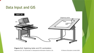
Data Input andGIS – Digitization & Scanning
Digitizing is a process of entering digital codes of analyzed data
into computer.
Digitizing can be manual (using digitizing tablet) or automatic
(using scanner).
The difference between two methods is that digitizing tablet
allows to do georeferencing during the digitizing process, while
scanning require georeferencing later, after digital file (usually
TIFF, GIF or JPEG image) has been created.
Another difference between methods is speed and accuracy of
the data processing.
Apparent slowness of the work on digitizing tablet compensates
often for the amount of editing after scanning process.
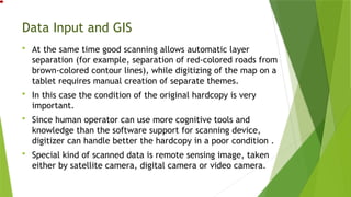
Data Input andGIS
At the same time good scanning allows automatic layer
separation (for example, separation of red-colored roads from
brown-colored contour lines), while digitizing of the map on a
tablet requires manual creation of separate themes.
In this case the condition of the original hardcopy is very
important.
Since human operator can use more cognitive tools and
knowledge than the software support for scanning device,
digitizer can handle better the hardcopy in a poor condition .
Special kind of scanned data is remote sensing image, taken
either by satellite camera, digital camera or video camera.
94.
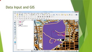
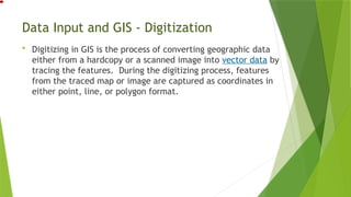
Data Input andGIS - Digitization
Digitizing in GIS is the process of converting geographic data
either from a hardcopy or a scanned image into vector data by
tracing the features. During the digitizing process, features
from the traced map or image are captured as coordinates in
either point, line, or polygon format.
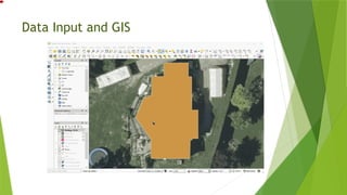
95.
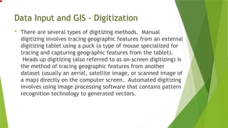
Data Input andGIS - Digitization
There are several types of digitizing methods. Manual
digitizing involves tracing geographic features from an external
digitizing tablet using a puck (a type of mouse specialized for
tracing and capturing geographic features from the tablet).
Heads up digitizing (also referred to as on-screen digitizing) is
the method of tracing geographic features from another
dataset (usually an aerial, satellite image, or scanned image of
a map) directly on the computer screen. Automated digitizing
involves using image processing software that contains pattern
recognition technology to generated vectors.
96.
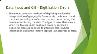
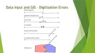
Data Input andGIS – Digitization Errors
Since most common methods of digitizing involve the
interpretation of geographic features via the human hand,
there are several types of errors that can occur during the
course of capturing the data. The type of error that occurs
when the feature is not captured properly is called a
positional error, as opposed to attribute errors where
information about the feature capture is inaccurate or false.
97.
Data Input andGIS – Digitization Errors
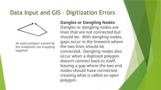
An open polygon caused by
the endpoints not snapping
together.
Dangles or Dangling Nodes
Dangles or dangling nodes are
lines that are not connected but
should be. With dangling nodes,
gaps occur in the linework where
the two lines should be
connected. Dangling nodes also
occur when a digitized polygon
doesn’t connect back to itself,
leaving a gap where the two end
nodes should have connected,
creating what is called an open
polygon.
98.
Data Input andGIS – Digitization Errors
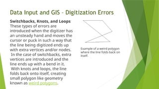
Example of a weird polygon
where the line folds back on
itself.
Switchbacks, Knots, and Loops
These types of errors are
introduced when the digitizer has
an unsteady hand and moves the
cursor or puck in such a way that
the line being digitized ends up
with extra vertices and/or nodes.
In the case of switchbacks, extra
vertices are introduced and the
line ends up with a bend in it.
With knots and loops, the line
folds back onto itself, creating
small polygon like geometry
known as weird polygons.
99.
Data Input andGIS – Digitization Errors
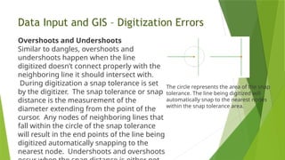
The circle represents the area of the snap
tolerance. The line being digitized will
automatically snap to the nearest nodes
within the snap tolerance area.
Overshoots and Undershoots
Similar to dangles, overshoots and
undershoots happen when the line
digitized doesn’t connect properly with the
neighboring line it should intersect with.
During digitization a snap tolerance is set
by the digitizer. The snap tolerance or snap
distance is the measurement of the
diameter extending from the point of the
cursor. Any nodes of neighboring lines that
fall within the circle of the snap tolerance
will result in the end points of the line being
digitized automatically snapping to the
nearest node. Undershoots and overshoots
100.
Data Input andGIS – Digitization Errors
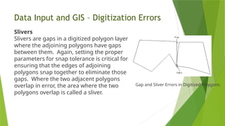
Slivers
Slivers are gaps in a digitized polygon layer
where the adjoining polygons have gaps
between them. Again, setting the proper
parameters for snap tolerance is critical for
ensuring that the edges of adjoining
polygons snap together to eliminate those
gaps. Where the two adjacent polygons
overlap in error, the area where the two
polygons overlap is called a sliver.
Gap and Sliver Errors in Digitized Polygons
Data Input andGIS – Scanners
Scanning coverts paper maps into digital format by
capturing features as individual cells, or pixels, producing
an automated image.
Maps are generally considered the backbone of any GIS
activity.
But many a time paper maps are not easily available in a
form that can be readily used by the computers.
Most of the paper maps had been prepared on the basis of
old conventional surveys.
New maps can be produced using improved technologies but
this requires time as it increases the volume of work. Thus,
we have to resort to the available maps.
103.
Data Input andGIS – Scanners
These paper maps have to be first converted into a digital format
usable by the computer.
This is a critical step as the quality of the analog document must be
preserved in the transition to the computer domain.
The technology used for this kind of conversions is known as scanning
and the instrument used for this kind of operation is known as a
scanner.
A scanner can be thought of as an electronic input device that converts
analog information of a document like a map, photograph or an overlay
into a digital format that can be used by the computer. Scanning
automatically captures map features, text, and symbols as individual
cells, or pixels, and produces an automated image.
104.
Data Input andGIS – Working of a Scanner
The most important component inside a scanner is the
scanner head which can move along the length of the
scanner.
The scanner head contains either a charged-couple device
(CCD) sensor or a contact image (CIS) sensor.
A CCD consists of a number of photosensitive cells or pixels
packed together on a chip.
The most advanced large format scanners use CCD’s with
8000 pixels per chip for providing a very good image quality.
105.
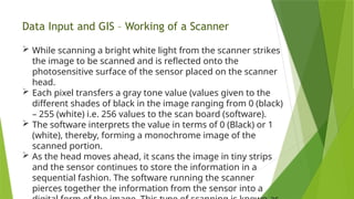
Data Input andGIS – Working of a Scanner
While scanning a bright white light from the scanner strikes
the image to be scanned and is reflected onto the
photosensitive surface of the sensor placed on the scanner
head.
Each pixel transfers a gray tone value (values given to the
different shades of black in the image ranging from 0 (black)
– 255 (white) i.e. 256 values to the scan board (software).
The software interprets the value in terms of 0 (Black) or 1
(white), thereby, forming a monochrome image of the
scanned portion.
As the head moves ahead, it scans the image in tiny strips
and the sensor continues to store the information in a
sequential fashion. The software running the scanner
pierces together the information from the sensor into a
106.
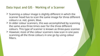
Data Input andGIS – Working of a Scanner
Scanning a colour image is slightly different in which the
scanner head has to scan the same image for three different
colours i.e. red, green, blue.
In older colour scanners, this was accomplished by scanning
the same area three times over for the three different
colours. This type of scanner is known as three-pass scanner.
However, most of the colour scanners now scan in one pass
scanning all the three colours in one go by using colour
filters.
107.
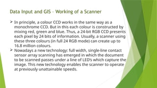
Data Input andGIS – Working of a Scanner
In principle, a colour CCD works in the same way as a
monochrome CCD. But in this each colour is constructed by
mixing red, green and blue. Thus, a 24-bit RGB CCD presents
each pixel by 24 bits of information. Usually, a scanner using
these three colours (in full 24 RGB mode) can create up to
16.8 million colours.
Nowadays a new technology: full width, single-line contact
sensor array scanning has emerged in which the document
to be scanned passes under a line of LED’s which capture the
image. This new technology enables the scanner to operate
at previously unattainable speeds.
108.
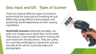
Data Input andGIS – Types of Scanner
There are several different types of scanners
performing the same job but handling the job
differently using different technologies and
producing results depending on their varying
capabilities.
Hand-held scanners although portable, can
only scan images up to about four inches wide.
They require a very steady hand for moving the
scan head over the document. They are useful
for scanning small logos or signatures and are
virtually of no use for scanning maps and
photographs.
109.
Data Input andGIS – Types of Scanner
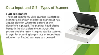
Flatbed scanners
The most commonly used scanner is a flatbed
scanner also known as desktop scanner. It has
a glass plate on which the picture or the
document is placed. The scanner head placed
beneath the glass plate moves across the
picture and the result is a good quality scanned
image. For scanning large maps or toposheets
wide format flatbed scanners can be used.
110.
Data Input andGIS – Types of Scanner
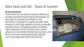
Drum scanners
Then there are the drum scanners which are
mostly used by the printing professionals. In
this type of scanner, the image or the
document is placed on a glass cylinder that
rotates at very high speeds around a centrally
located sensor containing photo-multiplier
tube instead of a CCD to scan. Prior to the
advances in the field of sheet fed scanners, the
drum scanners were extensively used for
scanning maps and other documents.
111.
Data Input andGIS – Types of Scanner
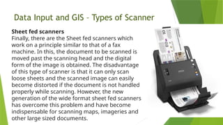
Sheet fed scanners
Finally, there are the Sheet fed scanners which
work on a principle similar to that of a fax
machine. In this, the document to be scanned is
moved past the scanning head and the digital
form of the image is obtained. The disadvantage
of this type of scanner is that it can only scan
loose sheets and the scanned image can easily
become distorted if the document is not handled
properly while scanning. However, the new
generation of the wide format sheet fed scanners
has overcome this problem and have become
indispensable for scanning maps, imageries and
other large sized documents.