Download as PDF, PPTX


![CSS SELECTORS
pe cd {
r, oe
fn-aiy "el" mnsae
otfml: Mno, oopc;
fn-ie 4p;
otsz: 8x
}
CSS style selectors
#o
fo / <n i=fo>
/ ay d"o"
fo
o / <o>
/ fo
.o
fo / <n cas"o"
/ ay ls=fo>
[o=a]
fobr / <n fo"a"
/ ay o=br>
fobr
o a / <o>br<fo
/ fo<a>/o>
fobr
o.a / <o cas"a"
/ fo ls=br>
fobr
o#a / <o i=br>
/ fo d"a"](https://image.slidesharecdn.com/d3workshop-130301204538-phpapp02/85/D3-js-workshop-22-320.jpg)

![DATA
Numbers
/ Abrcat pras
/ a hr, ehp?
vrdt =[,1 2 3 5 8;
a aa 1 , , , , ]
Objects
/ Asatrlt pras
/ ctepo, ehp?
vrdt =[
a aa
{:1.,y 91}
x 00 : .4,
{: 80 y 81}
x ., : .4,
{:1.,y 87}
x 30 : .4,
{: 90 y 87}
x ., : .7,
{:1.,y 92}
x 10 : .6
];](https://image.slidesharecdn.com/d3workshop-130301204538-phpapp02/85/D3-js-workshop-30-320.jpg)


![/ Asatrlt pras
/ ctepo, ehp?
vrdt =[
a aa
{ae "lc" x 1.,y 91}
nm: Aie, : 00 : .4,
{ae
nm: "o" x 80 y 81}
Bb, : ., : .4,
{ae "ao" x 1.,y 87}
nm: Crl, : 30 : .4,
{ae "ae,x 90 y 87}
nm: Dv" : ., : .7,
{ae "dt" x 1.,y 92}
nm: Eih, : 10 : .6
];
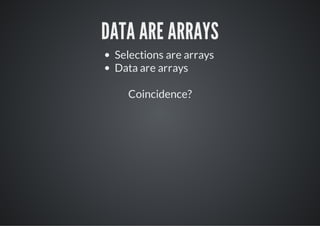
If needed, data should have a unique key for joining.](https://image.slidesharecdn.com/d3workshop-130301204538-phpapp02/85/D3-js-workshop-45-320.jpg)
![vrx=d.cl.ier)
a 3saelna(
.oan[2 2]
dmi(1, 4)
.ag(0 70)
rne[, 2];
x1) / 20
(6; / 4
vrx=d.cl.qt)
a 3saesr(
.oan[2 2]
dmi(1, 4)
.ag(0 70)
rne[, 2];
x1) / 289592053
(6; / 6.069638
vrx=d.cl.o(
a 3saelg)
.oan[2 2]
dmi(1, 4)
.ag(0 70)
rne[, 2];
x1) / 288694063
(6; / 9.2998777](https://image.slidesharecdn.com/d3workshop-130301204538-phpapp02/85/D3-js-workshop-54-320.jpg)
![vrx=d.cl.ier)
a 3saelna(
.oan[,d.a(ubr))
dmi(0 3mxnmes]
.ag(0 70)
rne[, 2];
vrx=d.cl.o(
a 3saelg)
.oand.xetnmes)
dmi(3etn(ubr)
.ag(0 70)
rne[, 2];
fnto vled {rtr dvle }
ucin au() eun .au;
vrx=d.cl.o(
a 3saelg)
.oand.xetojcs vle)
dmi(3etn(bet, au)
.ag(0 70)
rne[, 2];](https://image.slidesharecdn.com/d3workshop-130301204538-phpapp02/85/D3-js-workshop-56-320.jpg)
![vrx=d.cl.ier)
a 3saelna(
.oan[2 2]
dmi(1, 4)
.ag("tebu" "rw")
rne[selle, bon];
x1) / #656
(6; / 668
vrx=d.cl.ier)
a 3saelna(
.oan[2 2]
dmi(1, 4)
.ag("p" "2p")
rne[0x, 70x];
x1) / 20x
(6; / 4p
vrx=d.cl.ier)
a 3saelna(
.oan[2 2]
dmi(1, 4)
.ag("tebu" "rw")
rne[selle, bon]
.neplt(3itroaes)
itroaed.nepltHl;
x1) / #c0f
(6; / 3b5](https://image.slidesharecdn.com/d3workshop-130301204538-phpapp02/85/D3-js-workshop-58-320.jpg)
![DIVERGING SCALES
Sometimes, you want a compound (“polylinear”) scale.
vrx=d.cl.ier)
a 3saelna(
.oan[1,0 10)
dmi(-0 , 0]
.ag("e" "ht" "re")
rne[rd, wie, gen];
x-) / #f00
(5; / f88
x5) / #000
(0; / 8c8](https://image.slidesharecdn.com/d3workshop-130301204538-phpapp02/85/D3-js-workshop-60-320.jpg)
![ORDINAL SCALES
An ordinal scale is essentially an explicit mapping.
vrx=d.cl.ria(
a 3saeodnl)
.oan[A,"" "" "")
dmi("" B, C, D]
.ag(0 1,2,3];
rne[, 0 0 0)
x"";/ 1
(B) / 0](https://image.slidesharecdn.com/d3workshop-130301204538-phpapp02/85/D3-js-workshop-61-320.jpg)
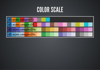
![vrx=d.cl.aeoy0)
a 3saectgr2(
.oan[A,"" "" "")
dmi("" B, C, D];
x"";/ #e78
(B) / ace
vrx=d.cl.aeoy0)
a 3saectgr2(
.oan[A,"" "" "")
dmi("" B, C, D];
x"";/ #c0c
(E) / 2a2
x"";/ #c0c
(E) / 2a2
xdmi(;/ A B C D E
.oan) / , , , ,](https://image.slidesharecdn.com/d3workshop-130301204538-phpapp02/85/D3-js-workshop-62-320.jpg)
![Ordinal ranges can be derived from continuous ranges.
vrx=d.cl.ria(
a 3saeodnl)
.oan[A,"" "" "")
dmi("" B, C, D]
.agPit(0 70)
rneons[, 2];
x"";/ 20
(B) / 4
vrx=d.cl.ria(
a 3saeodnl)
.oan[A,"" "" "")
dmi("" B, C, D]
.agRudad(0 70,.)
rneonBns[, 2] 2;
x"";/ 26 brpsto
(B) / 0, a oiin
xrnead) / 17 brwdh
.agBn(; / 3, a it](https://image.slidesharecdn.com/d3workshop-130301204538-phpapp02/85/D3-js-workshop-64-320.jpg)
![TICKS
Quantitative scales can be queried for “human-readable”
values.
vrx=d.cl.ier)
a 3saelna(
.oan[2 2]
dmi(1, 4)
.ag(0 70)
rne[, 2];
xtcs5;/ [2 1,1,1,2,2,2]
.ik() / 1, 4 6 8 0 2 4
The requested count is only a hint (for better or worse).](https://image.slidesharecdn.com/d3workshop-130301204538-phpapp02/85/D3-js-workshop-69-320.jpg)


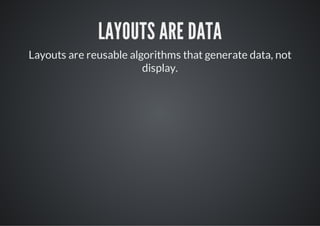
![Layouts are configurable functions.
vrtemp=d.aottemp)
a rea 3lyu.rea(
.adn()
pdig4
.ie[it,hih];
sz(wdh egt)](https://image.slidesharecdn.com/d3workshop-130301204538-phpapp02/85/D3-js-workshop-93-320.jpg)

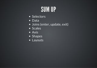


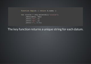
This document provides an overview of key concepts for working with D3, including: - D3 uses standard web technologies like HTML, SVG, and CSS rather than introducing new representations. Learning D3 largely means learning web standards. - Visualization with D3 requires mapping data to visual elements using scales. Scales are functions that map from data values to visual values like pixel positions. - Selections in D3 correspond to elements in the DOM. Data joins allow binding data to selections to drive attribute updates. The enter, update, exit pattern is used to handle new, existing and removed data. - Common scale types include linear, log, quantize and quantile for quantitative data, and


![Writing SOLID C++ [gbgcpp meetup @ Zenseact]](https://cdn.slidesharecdn.com/ss_thumbnails/writingsolidc2-211126183844-thumbnail.jpg?width=640&height=640&fit=bounds)


![[1062BPY12001] Data analysis with R / week 2](https://cdn.slidesharecdn.com/ss_thumbnails/dataanalyzer01-180307063046-thumbnail.jpg?width=640&height=640&fit=bounds)