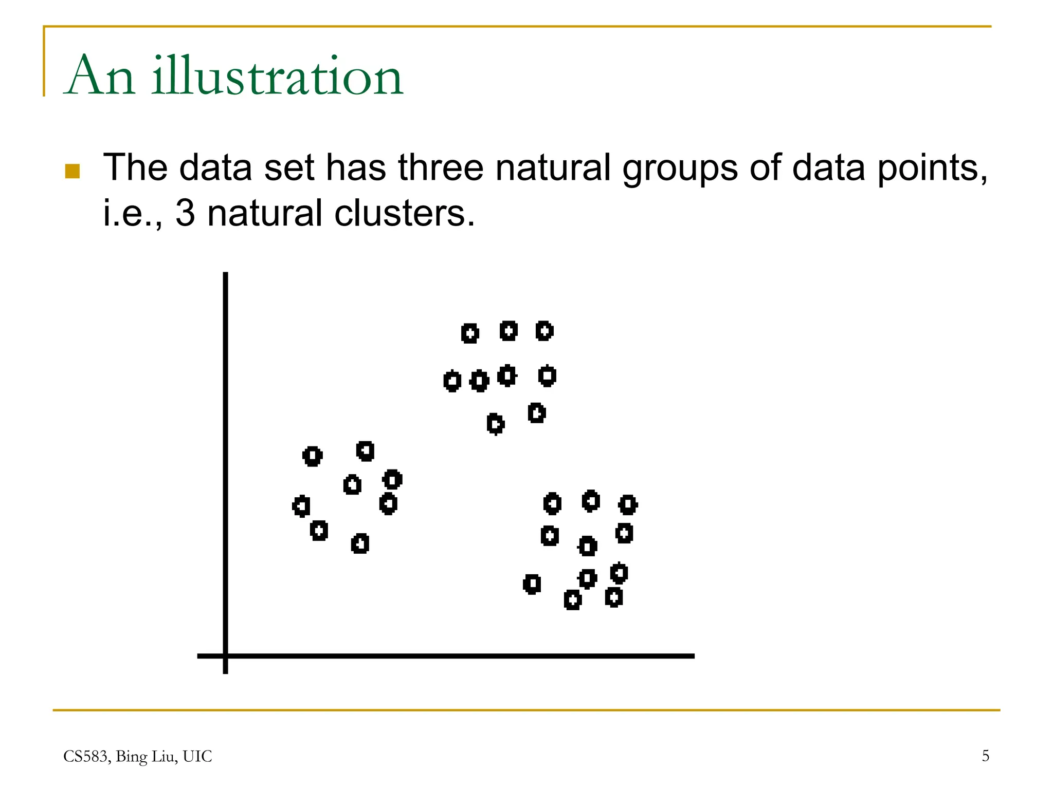
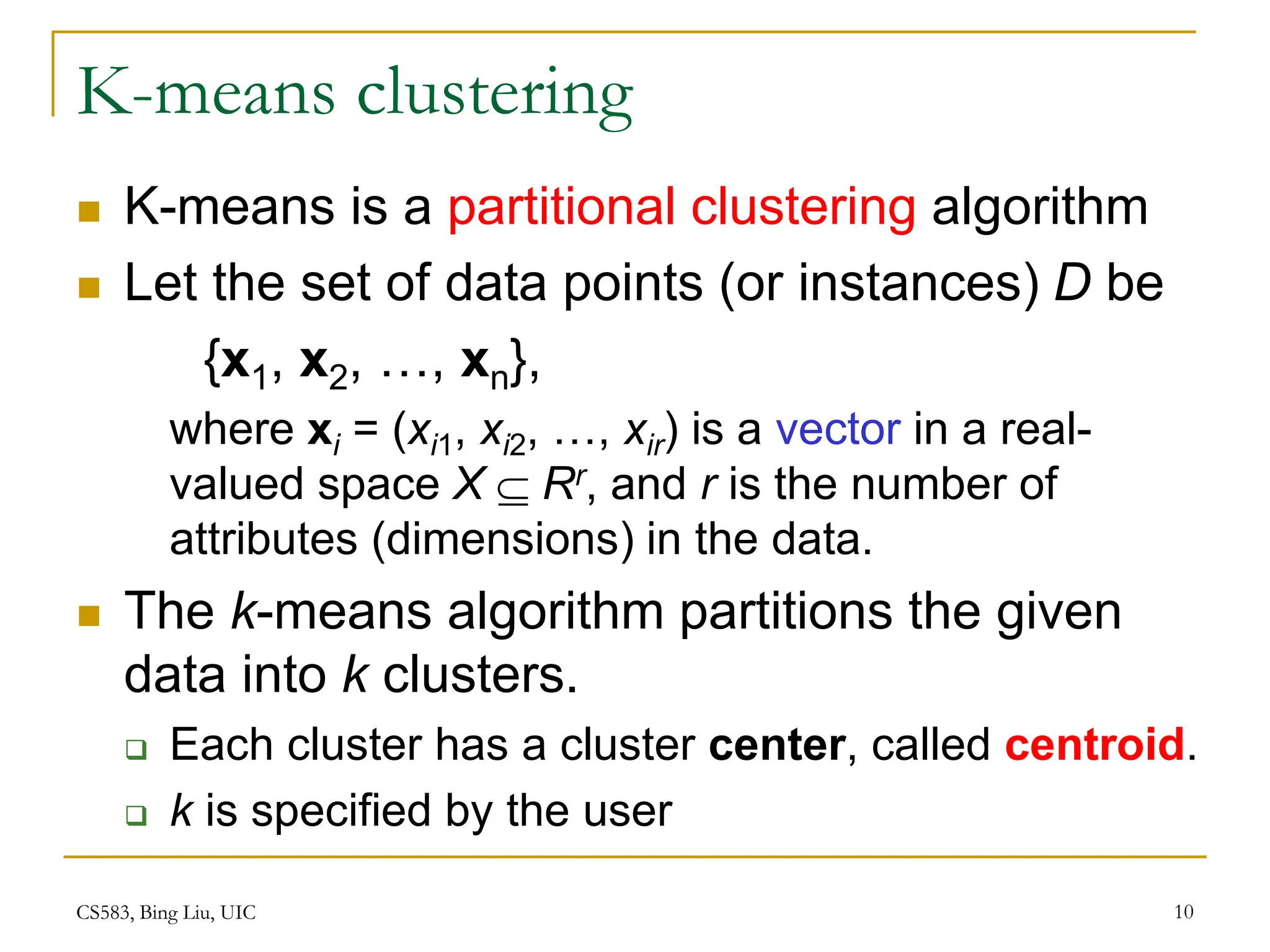
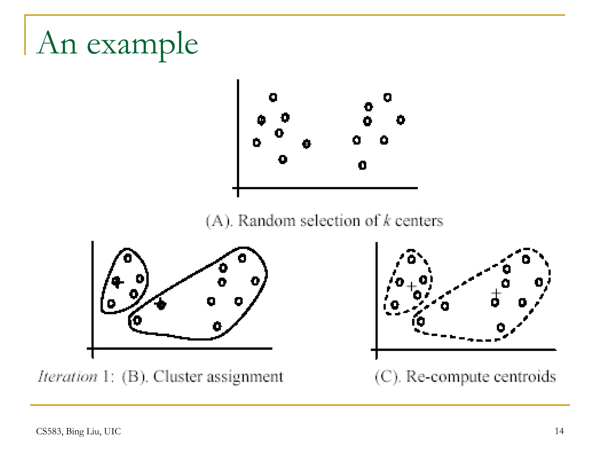
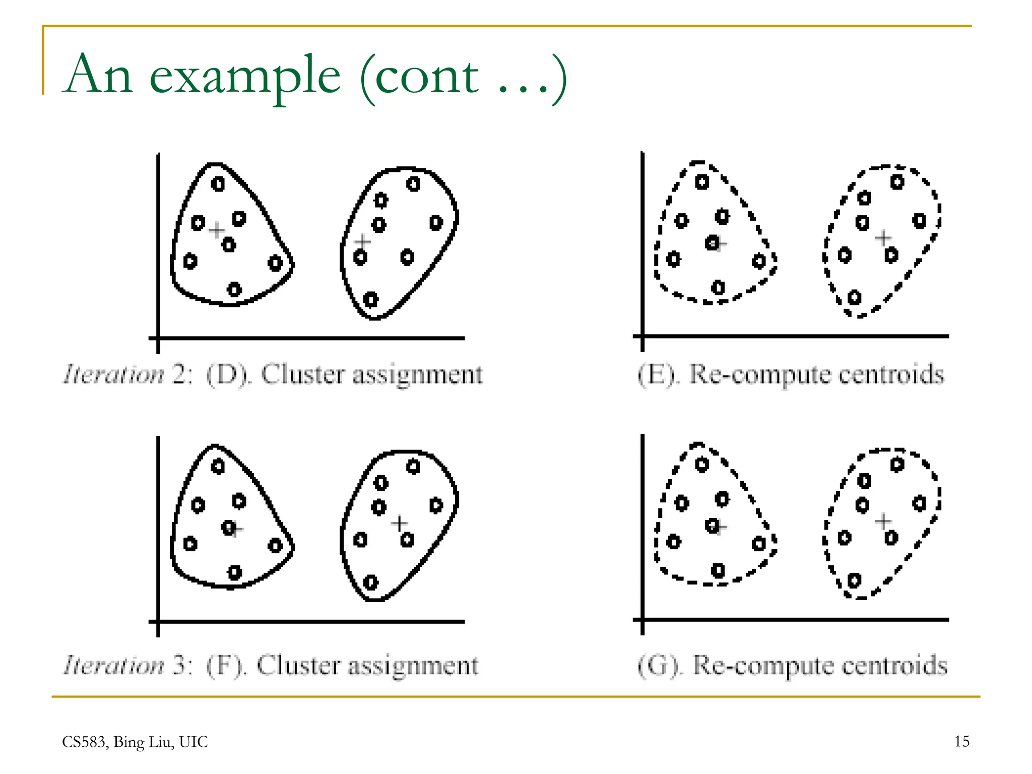
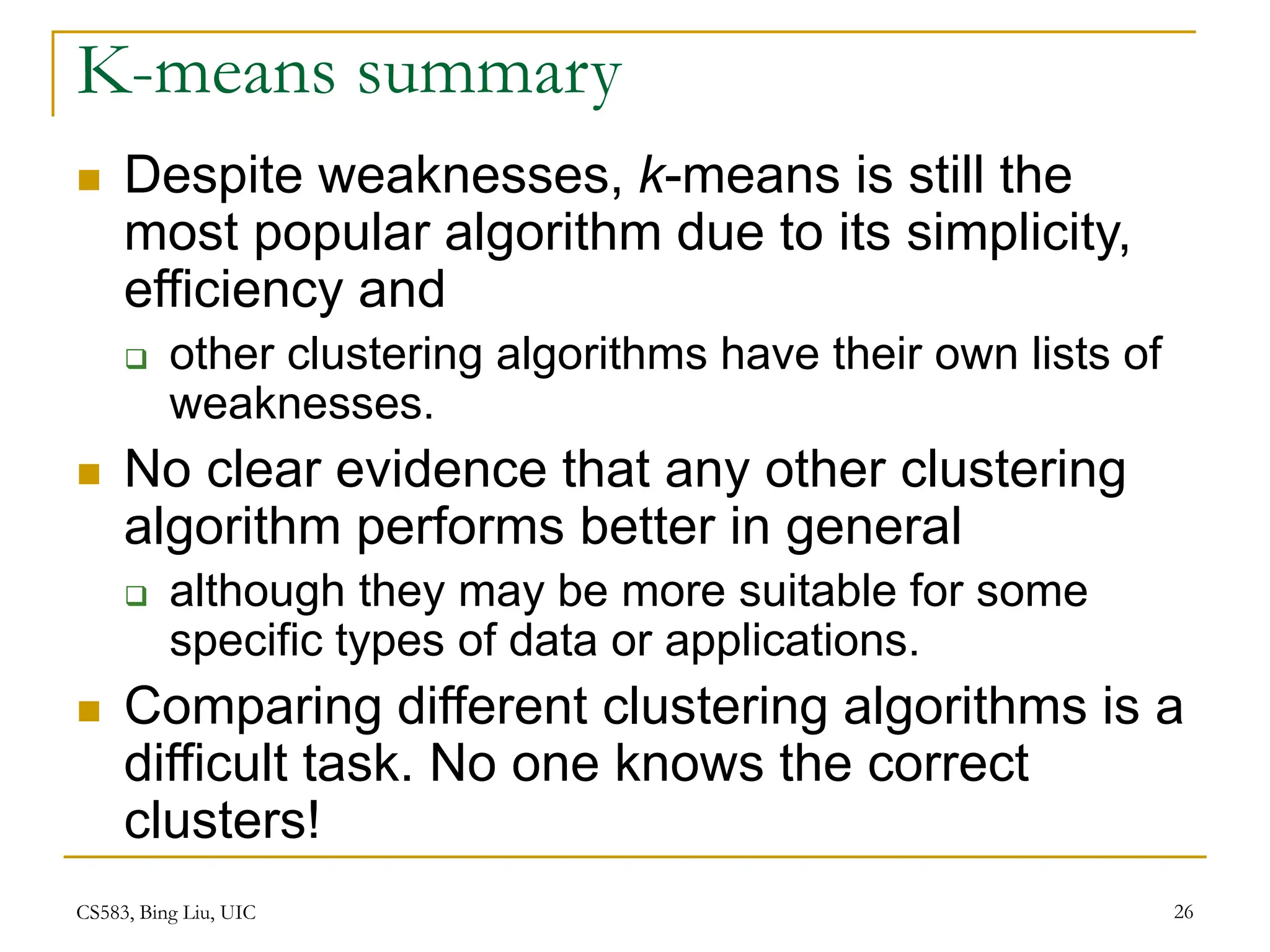
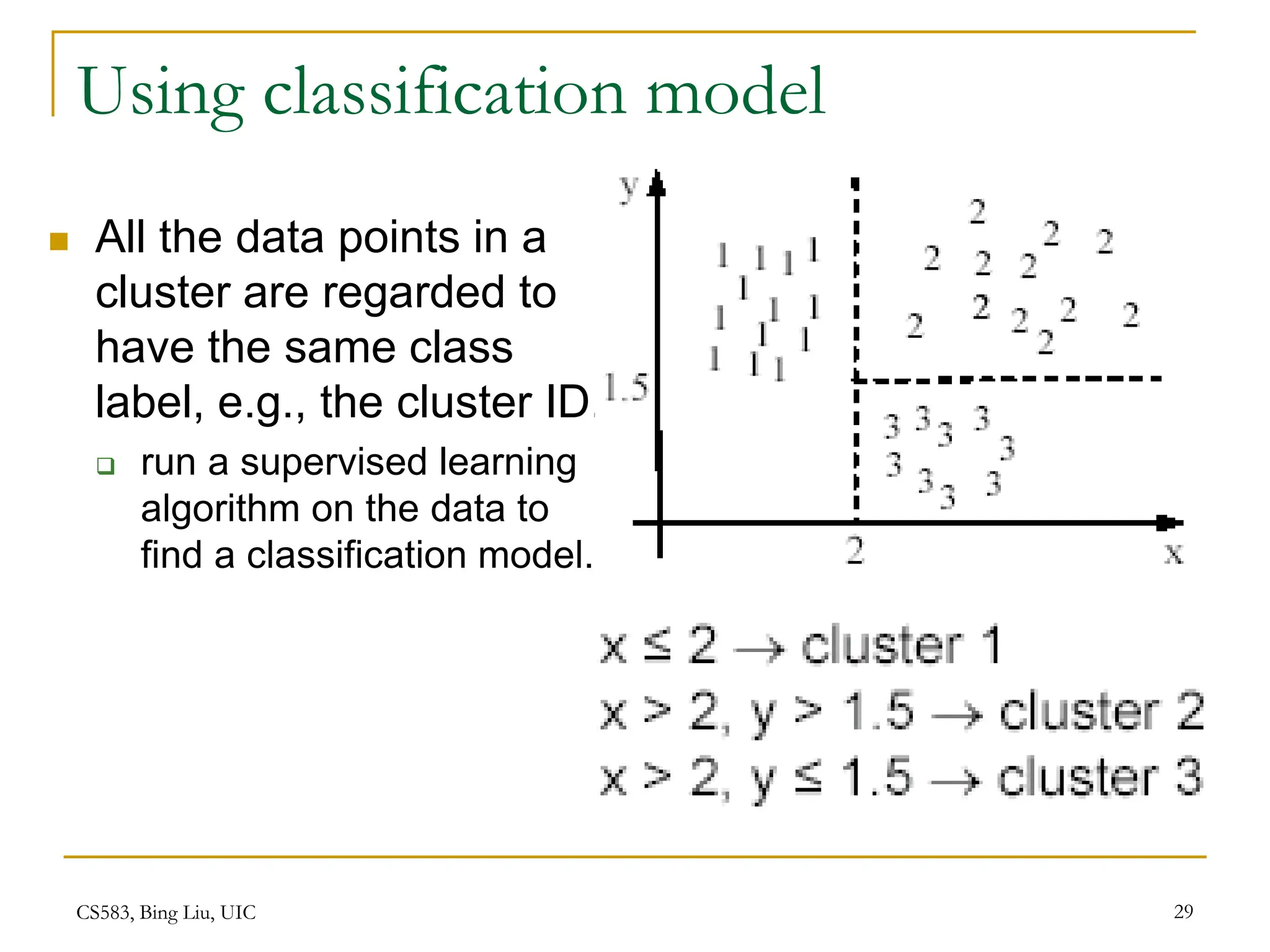
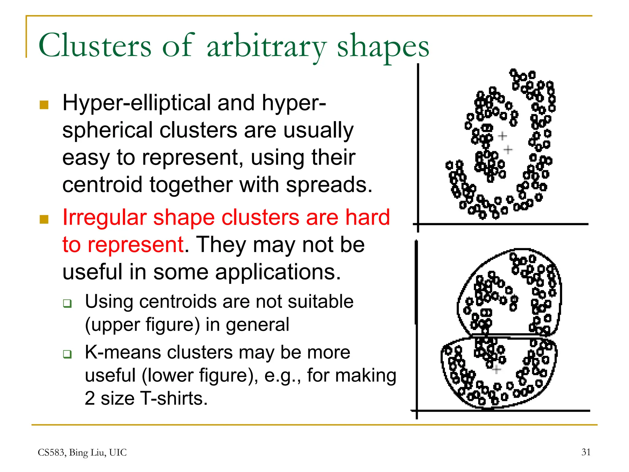
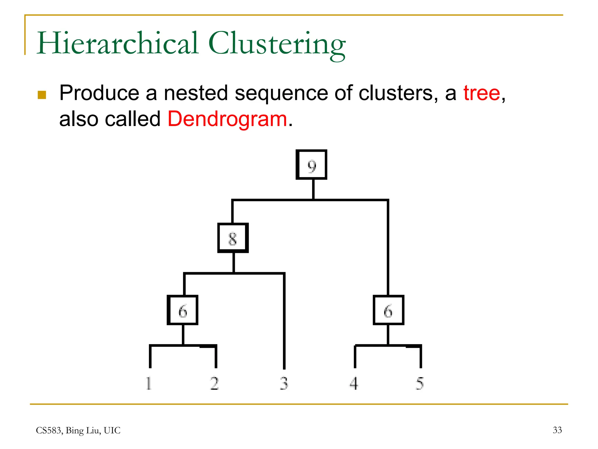
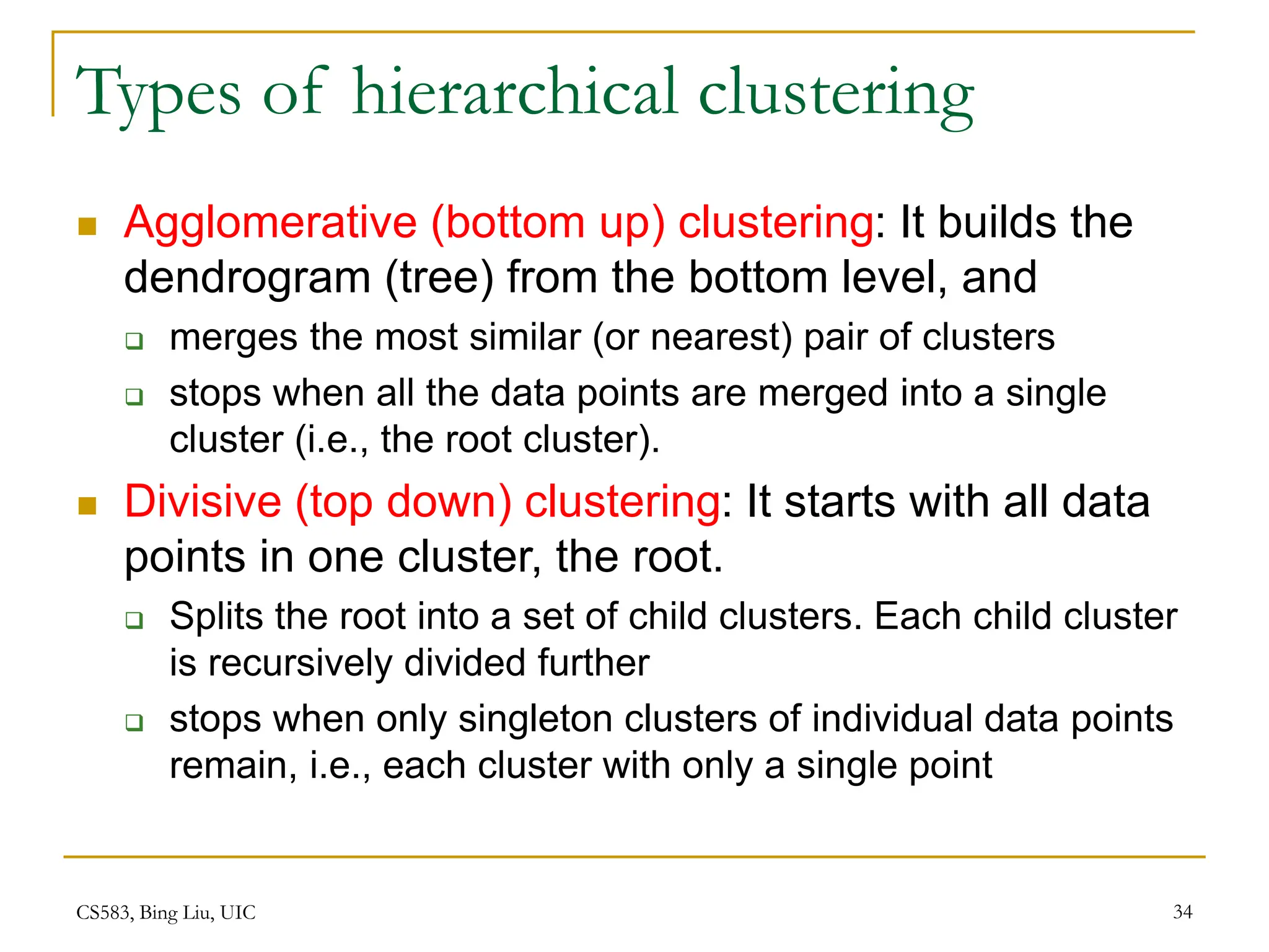
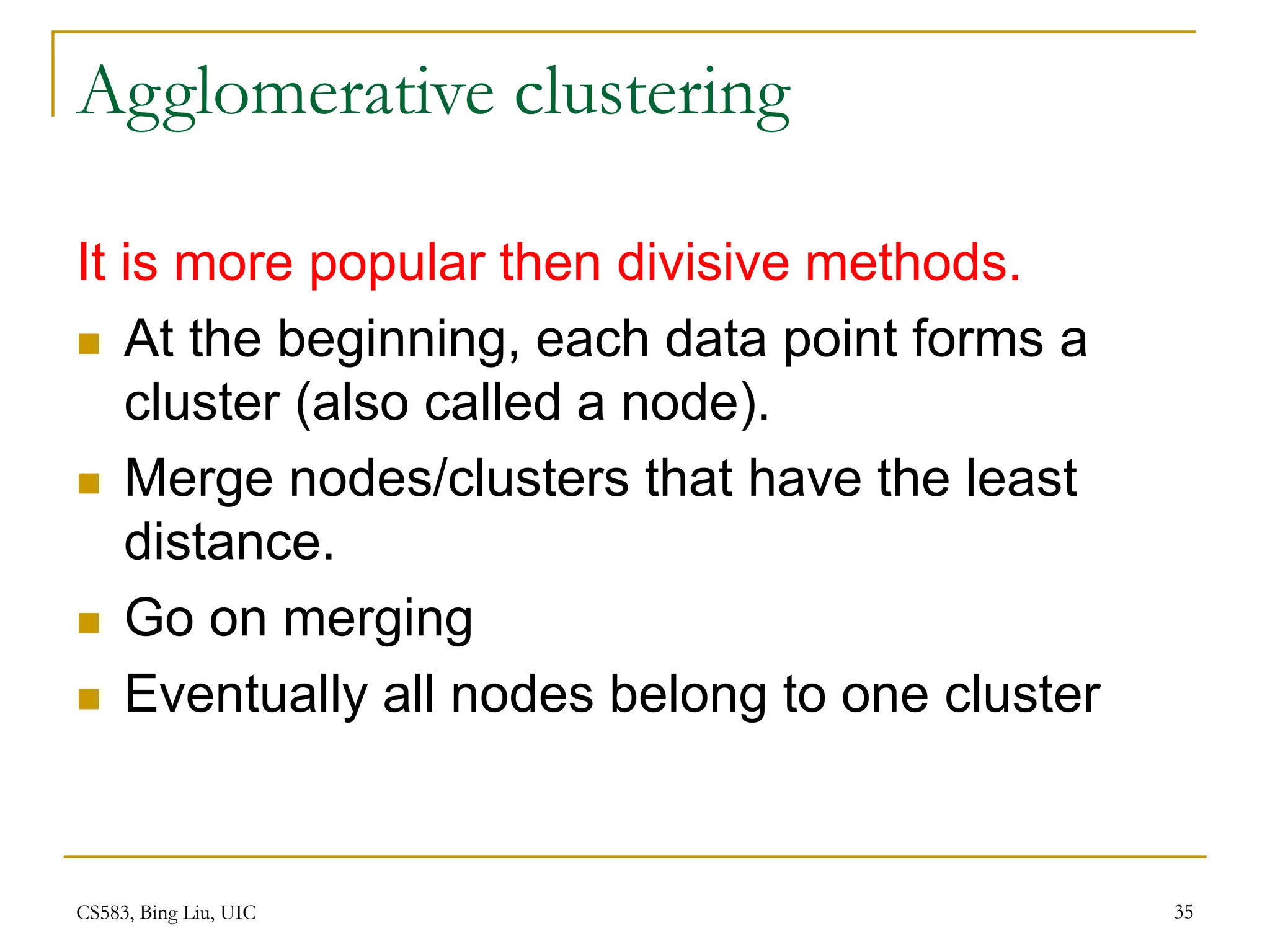
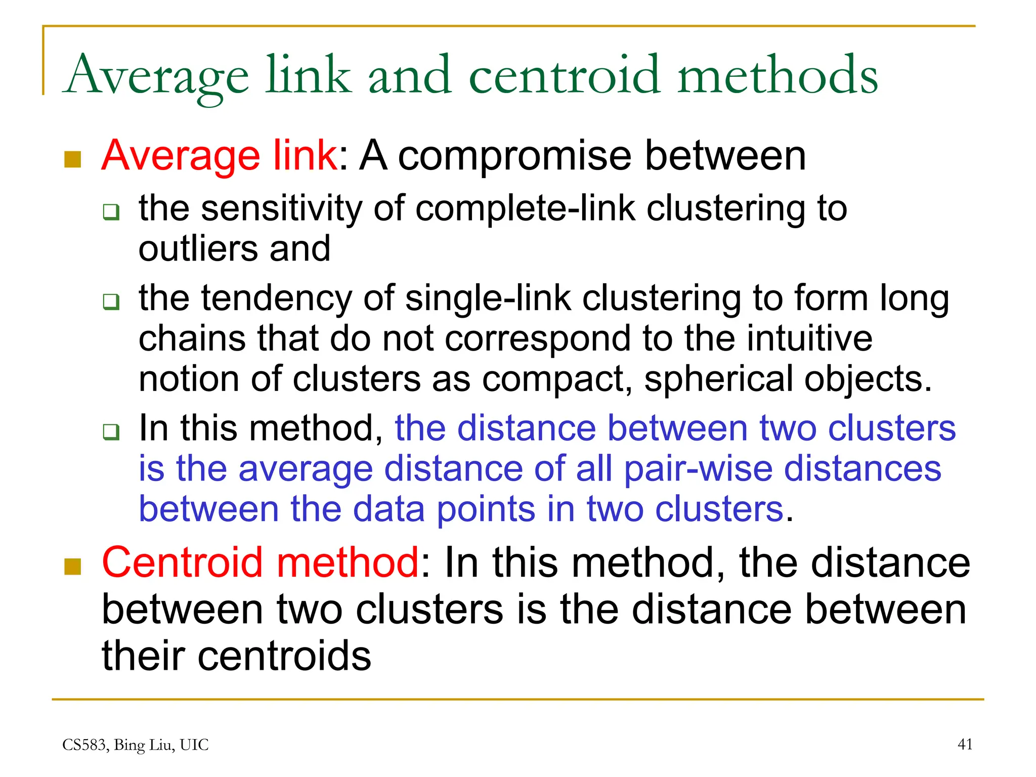
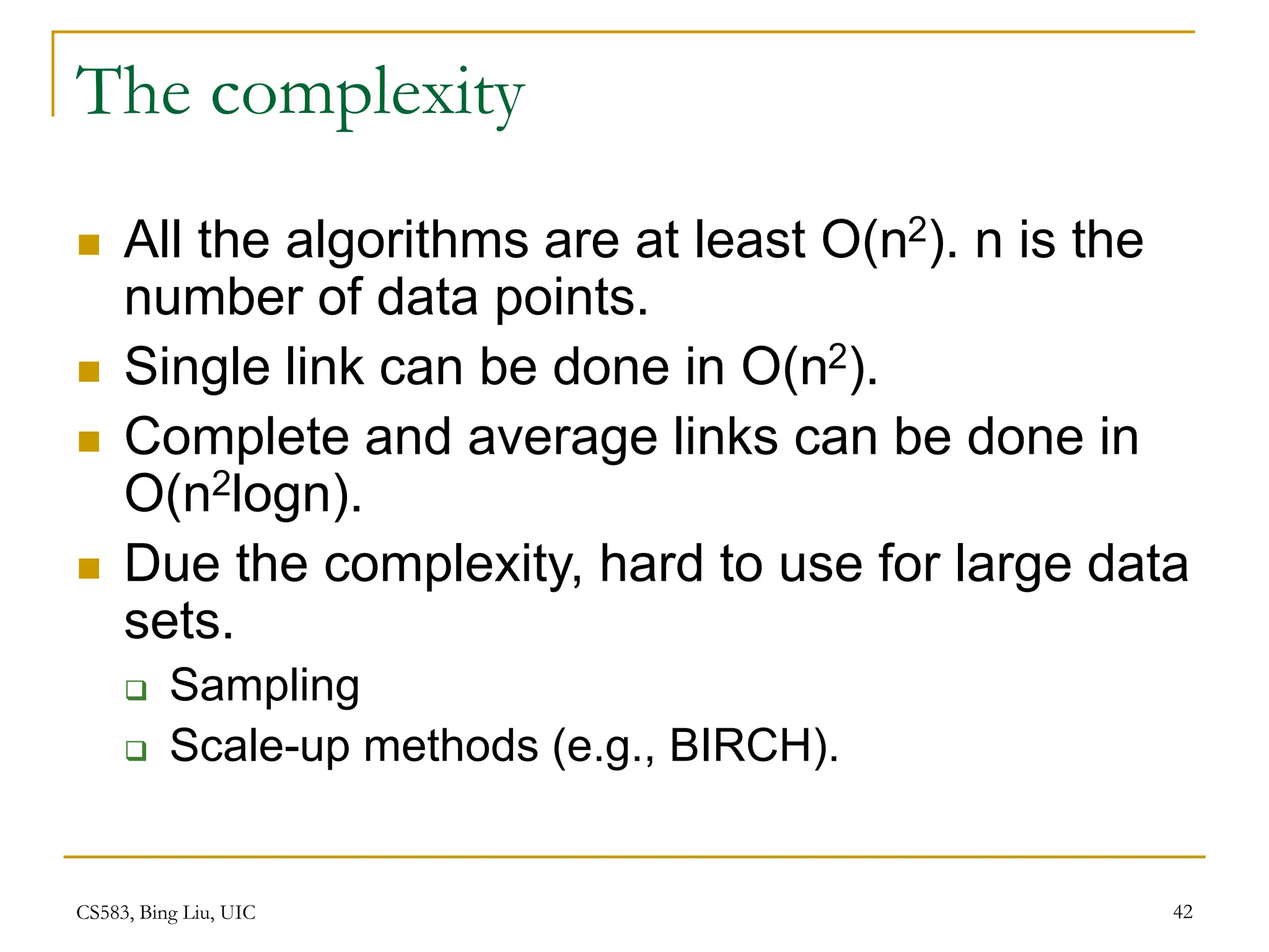
CS583-unsupervised-learning.ppt learning

Chapter 4:
Unsupervised Learning

CS583, Bing Liu, UIC 2
Road map
 Basic concepts
 K-means algorithm
 Representation of clusters
 Hierarchical clustering
 Distance functions
 Data standardization
 Handling mixed attributes
 Which clustering algorithm to use?
 Cluster evaluation
 Discovering holes and data regions
 Summary

Supervised learning vs. unsupervised
learning
 Supervised learning: discover patterns in the
data that relate data attributes with a target
(class) attribute.
 These patterns are then utilized to predict the
values of the target attribute in future data
instances.
 Unsupervised learning: The data have no
target attribute.
 We want to explore the data to find some intrinsic
structures in them.

Clustering
 Clustering is a technique for finding similarity groups
in data, called clusters. I.e.,
 it groups data instances that are similar to (near) each other
in one cluster and data instances that are very different (far
away) from each other into different clusters.
 Clustering is often called an unsupervised learning
task as no class values denoting an a priori grouping
of the data instances are given, which is the case in
supervised learning.
 Due to historical reasons, clustering is often
considered synonymous with unsupervised learning.
 In fact, association rule mining is also unsupervised
 This chapter focuses on clustering.

An illustration
 The data set has three natural groups of data points,
i.e., 3 natural clusters.

What is clustering for?
 Let us see some real-life examples
 Example 1: groups people of similar sizes
together to make “small”, “medium” and
“large” T-Shirts.
 Tailor-made for each person: too expensive
 One-size-fits-all: does not fit all.
 Example 2: In marketing, segment customers
according to their similarities
 To do targeted marketing.

What is clustering for? (cont…)
 Example 3: Given a collection of text
documents, we want to organize them
according to their content similarities,
 To produce a topic hierarchy
 In fact, clustering is one of the most utilized
data mining techniques.
 It has a long history, and used in almost every
field, e.g., medicine, psychology, botany, sociology,
biology, archeology, marketing, insurance,
libraries, etc.
 In recent years, due to the rapid increase of online
documents, text clustering becomes important.

Aspects of clustering
 A clustering algorithm
 Partitional clustering
 Hierarchical clustering
 …
 A distance (similarity, or dissimilarity) function
 Clustering quality
 Inter-clusters distance  maximized
 Intra-clusters distance  minimized
 The quality of a clustering result depends on
the algorithm, the distance function, and the
application.

Road map
 Basic concepts
 Summary

K-means clustering
 K-means is a partitional clustering algorithm
 Let the set of data points (or instances) D be
{x1, x2, …, xn},
where xi = (xi1, xi2, …, xir) is a vector in a real-
valued space X  Rr, and r is the number of
attributes (dimensions) in the data.
 The k-means algorithm partitions the given
data into k clusters.
 Each cluster has a cluster center, called centroid.
 k is specified by the user

K-means algorithm
 Given k, the k-means algorithm works as
follows:
1)Randomly choose k data points (seeds) to be the
initial centroids, cluster centers
2)Assign each data point to the closest centroid
3)Re-compute the centroids using the current
cluster memberships.
4)If a convergence criterion is not met, go to 2).

K-means algorithm – (cont …)

Stopping/convergence criterion
1. no (or minimum) re-assignments of data
points to different clusters,
2. no (or minimum) change of centroids, or
3. minimum decrease in the sum of squared
error (SSE),
 Ci is the jth cluster, mj is the centroid of cluster Cj
(the mean vector of all the data points in Cj), and
dist(x, mj) is the distance between data point x
and centroid mj.




k
j
C j
j
dist
SSE
1
2
)
,
(
x
m
x (1)

An example
+
+

An example (cont …)

An example distance function

A disk version of k-means
 K-means can be implemented with data on
disk
 In each iteration, it scans the data once.
 as the centroids can be computed incrementally
 It can be used to cluster large datasets that
do not fit in main memory
 We need to control the number of iterations
 In practice, a limited is set (< 50).
 Not the best method. There are other scale-
up algorithms, e.g., BIRCH.

A disk version of k-means (cont …)

Strengths of k-means
 Strengths:
 Simple: easy to understand and to implement
 Efficient: Time complexity: O(tkn),
where n is the number of data points,
k is the number of clusters, and
t is the number of iterations.
 Since both k and t are small. k-means is considered a
linear algorithm.
 K-means is the most popular clustering algorithm.
 Note that: it terminates at a local optimum if SSE is
used. The global optimum is hard to find due to
complexity.

Weaknesses of k-means
 The algorithm is only applicable if the mean is
defined.
 For categorical data, k-mode - the centroid is
represented by most frequent values.
 The user needs to specify k.
 The algorithm is sensitive to outliers
 Outliers are data points that are very far away
from other data points.
 Outliers could be errors in the data recording or
some special data points with very different values.

Weaknesses of k-means: Problems with
outliers

Weaknesses of k-means: To deal with
outliers
 One method is to remove some data points in the
clustering process that are much further away from
the centroids than other data points.
 To be safe, we may want to monitor these possible outliers
over a few iterations and then decide to remove them.
 Another method is to perform random sampling.
Since in sampling we only choose a small subset of
the data points, the chance of selecting an outlier is
very small.
 Assign the rest of the data points to the clusters by
distance or similarity comparison, or classification

Weaknesses of k-means (cont …)
 The algorithm is sensitive to initial seeds.

 If we use different seeds: good results
 There are some
methods to help
choose good
seeds

 The k-means algorithm is not suitable for
discovering clusters that are not hyper-ellipsoids (or
hyper-spheres).
+

K-means summary
 Despite weaknesses, k-means is still the
most popular algorithm due to its simplicity,
efficiency and
 other clustering algorithms have their own lists of
weaknesses.
 No clear evidence that any other clustering
algorithm performs better in general
 although they may be more suitable for some
specific types of data or applications.
 Comparing different clustering algorithms is a
difficult task. No one knows the correct
clusters!

Road map
 Basic concepts
 Summary

Common ways to represent clusters
 Use the centroid of each cluster to represent
the cluster.
 compute the radius and
 standard deviation of the cluster to determine its
spread in each dimension
 The centroid representation alone works well if the
clusters are of the hyper-spherical shape.
 If clusters are elongated or are of other shapes,
centroids are not sufficient

Using classification model
 All the data points in a
cluster are regarded to
have the same class
label, e.g., the cluster ID.
 run a supervised learning
algorithm on the data to
find a classification model.

Use frequent values to represent cluster
 This method is mainly for clustering of
categorical data (e.g., k-modes clustering).
 Main method used in text clustering, where a
small set of frequent words in each cluster is
selected to represent the cluster.

Clusters of arbitrary shapes
 Hyper-elliptical and hyper-
spherical clusters are usually
easy to represent, using their
centroid together with spreads.
 Irregular shape clusters are hard
to represent. They may not be
useful in some applications.
 Using centroids are not suitable
(upper figure) in general
 K-means clusters may be more
useful (lower figure), e.g., for making
2 size T-shirts.

Road map
 Basic concepts
 Summary

Hierarchical Clustering
 Produce a nested sequence of clusters, a tree,
also called Dendrogram.

Types of hierarchical clustering
 Agglomerative (bottom up) clustering: It builds the
dendrogram (tree) from the bottom level, and
 merges the most similar (or nearest) pair of clusters
 stops when all the data points are merged into a single
cluster (i.e., the root cluster).
 Divisive (top down) clustering: It starts with all data
points in one cluster, the root.
 Splits the root into a set of child clusters. Each child cluster
is recursively divided further
 stops when only singleton clusters of individual data points
remain, i.e., each cluster with only a single point

Agglomerative clustering
It is more popular then divisive methods.
 At the beginning, each data point forms a
cluster (also called a node).
 Merge nodes/clusters that have the least
distance.
 Go on merging
 Eventually all nodes belong to one cluster

Agglomerative clustering algorithm

An example: working of the algorithm

Measuring the distance of two clusters
 A few ways to measure distances of two
clusters.
 Results in different variations of the algorithm.
 Single link
 Complete link
 Average link
 Centroids
 …

Single link method
 The distance between
two clusters is the
distance between two
closest data points in
the two clusters, one
data point from each
cluster.
 It can find arbitrarily
shaped clusters, but
 It may cause the
undesirable “chain effect”
by noisy points
Two natural clusters are
split into two

Complete link method
 The distance between two clusters is the distance
of two furthest data points in the two clusters.
 It is sensitive to outliers because they are far
away

Average link and centroid methods
 Average link: A compromise between
 the sensitivity of complete-link clustering to
outliers and
 the tendency of single-link clustering to form long
chains that do not correspond to the intuitive
notion of clusters as compact, spherical objects.
 In this method, the distance between two clusters
is the average distance of all pair-wise distances
between the data points in two clusters.
 Centroid method: In this method, the distance
between two clusters is the distance between
their centroids

The complexity
 All the algorithms are at least O(n2). n is the
number of data points.
 Single link can be done in O(n2).
 Complete and average links can be done in
O(n2logn).
 Due the complexity, hard to use for large data
sets.
 Sampling
 Scale-up methods (e.g., BIRCH).

Road map
 Basic concepts
 Summary

Distance functions
 Key to clustering. “similarity” and “dissimilarity”
can also commonly used terms.
 There are numerous distance functions for
 Different types of data
 Numeric data
 Nominal data
 Different specific applications

Distance functions for numeric attributes
 Most commonly used functions are
 Euclidean distance and
 Manhattan (city block) distance
 We denote distance with: dist(xi, xj), where xi
and xj are data points (vectors)
 They are special cases of Minkowski distance.
h is positive integer.
h
h
jr
ir
h
j
i
h
j
i
j
i x
x
x
x
x
x
dist
1
2
2
1
1 )
)
(
...
)
(
)
((
)
,
( 






x
x

Euclidean distance and Manhattan distance
 If h = 2, it is the Euclidean distance
 If h = 1, it is the Manhattan distance
 Weighted Euclidean distance
2
2
2
2
2
1
1 )
(
...
)
(
)
(
)
,
( jr
ir
j
i
j
i
j
i x
x
x
x
x
x
dist 






x
x
|
|
...
|
|
|
|
)
,
( 2
2
1
1 jr
ir
j
i
j
i
j
i x
x
x
x
x
x
dist 






x
x
2
2
2
2
2
2
1
1
1 )
(
...
)
(
)
(
)
,
( jr
ir
r
j
i
j
i
j
i x
x
w
x
x
w
x
x
w
dist 






x
x

Squared distance and Chebychev distance
 Squared Euclidean distance: to place
progressively greater weight on data points
that are further apart.
 Chebychev distance: one wants to define two
data points as "different" if they are different
on any one of the attributes.
2
2
2
2
2
1
1 )
(
...
)
(
)
(
)
,
( jr
ir
j
i
j
i
j
i x
x
x
x
x
x
dist 






x
x
|)
|
...,
|,
|
|,
max(|
)
,
( 2
2
1
1 jr
ir
j
i
j
i
j
i x
x
x
x
x
x
dist 



x
x

Distance functions for binary and
nominal attributes
 Binary attribute: has two values or states but
no ordering relationships, e.g.,
 Gender: male and female.
 We use a confusion matrix to introduce the
distance functions/measures.
 Let the ith and jth data points be xi and xj
(vectors)

Confusion matrix

Symmetric binary attributes
 A binary attribute is symmetric if both of its
states (0 and 1) have equal importance, and
carry the same weights, e.g., male and
female of the attribute Gender
 Distance function: Simple Matching
Coefficient, proportion of mismatches of their
values
d
c
b
a
c
b
dist j
i





)
,
( x
x

Symmetric binary attributes: example

Asymmetric binary attributes
 Asymmetric: if one of the states is more
important or more valuable than the other.
 By convention, state 1 represents the more
important state, which is typically the rare or
infrequent state.
 Jaccard coefficient is a popular measure
 We can have some variations, adding weights
c
b
a
c
b
dist j
i




)
,
( x
x

Nominal attributes
 Nominal attributes: with more than two states
or values.
 the commonly used distance measure is also
based on the simple matching method.
 Given two data points xi and xj, let the number of
attributes be r, and the number of values that
match in xi and xj be q.
r
q
r
dist j
i


)
,
( x
x

Distance function for text documents
 A text document consists of a sequence of
sentences and each sentence consists of a
sequence of words.
 To simplify: a document is usually considered a
“bag” of words in document clustering.
 Sequence and position of words are ignored.
 A document is represented with a vector just like a
normal data point.
 It is common to use similarity to compare two
documents rather than distance.
 The most commonly used similarity function is the cosine
similarity. We will study this later.

Road map
 Basic concepts
 Summary

Data standardization
 In the Euclidean space, standardization of attributes
is recommended so that all attributes can have
equal impact on the computation of distances.
 Consider the following pair of data points
 xi: (0.1, 20) and xj: (0.9, 720).
 The distance is almost completely dominated by
(720-20) = 700.
 Standardize attributes: to force the attributes to have
a common value range
,
700.000457
)
20
720
(
)
1
.
0
9
.
0
(
)
,
( 2
2





j
i
dist x
x

Interval-scaled attributes
 Their values are real numbers following a
linear scale.
 The difference in Age between 10 and 20 is the
same as that between 40 and 50.
 The key idea is that intervals keep the same
importance through out the scale
 Two main approaches to standardize interval
scaled attributes, range and z-score. f is an
attribute
,
)
min(
)
max(
)
min(
)
(
f
f
f
x
x
range
if
if




Interval-scaled attributes (cont …)
 Z-score: transforms the attribute values so that they
have a mean of zero and a mean absolute
deviation of 1. The mean absolute deviation of
attribute f, denoted by sf, is computed as follows
 ,
|
|
...
|
|
|
|
1
2
1 f
nf
f
f
f
f
f m
x
m
x
m
x
n
s 






 ,
...
1
2
1 nf
f
f
f x
x
x
n
m 



.
)
(
f
f
if
if
s
m
x
x
z


Z-score:

Ratio-scaled attributes
 Numeric attributes, but unlike interval-scaled
attributes, their scales are exponential,
 For example, the total amount of
microorganisms that evolve in a time t is
approximately given by
AeBt,
 where A and B are some positive constants.
 Do log transform:
 Then treat it as an interval-scaled attribuete
)
log( if
x

Nominal attributes
 Sometime, we need to transform nominal
attributes to numeric attributes.
 Transform nominal attributes to binary
attributes.
 The number of values of a nominal attribute is v.
 Create v binary attributes to represent them.
 If a data instance for the nominal attribute takes a
particular value, the value of its binary attribute is
set to 1, otherwise it is set to 0.
 The resulting binary attributes can be used as
numeric attributes, with two values, 0 and 1.

Nominal attributes: an example
 Nominal attribute fruit: has three values,
 Apple, Orange, and Pear
 We create three binary attributes called,
Apple, Orange, and Pear in the new data.
 If a particular data instance in the original
data has Apple as the value for fruit,
 then in the transformed data, we set the value of
the attribute Apple to 1, and
 the values of attributes Orange and Pear to 0

Ordinal attributes
 Ordinal attribute: an ordinal attribute is like a
nominal attribute, but its values have a
numerical ordering. E.g.,
 Age attribute with values: Young, MiddleAge and
Old. They are ordered.
 Common approach to standardization: treat is as
an interval-scaled attribute.

Road map
 Basic concepts
 Summary

Mixed attributes
 Our distance functions given are for data with
all numeric attributes, or all nominal attributes,
etc.
 Practical data has different types:
 Any subset of the 6 types of attributes,
 interval-scaled,
 symmetric binary,
 asymmetric binary,
 ratio-scaled,
 ordinal and
 nominal

Convert to a single type
 One common way of dealing with mixed
attributes is to
 Decide the dominant attribute type, and
 Convert the other types to this type.
 E.g, if most attributes in a data set are
interval-scaled,
 we convert ordinal attributes and ratio-scaled
attributes to interval-scaled attributes.
 It is also appropriate to treat symmetric binary
attributes as interval-scaled attributes.

Convert to a single type (cont …)
 It does not make much sense to convert a
nominal attribute or an asymmetric binary
attribute to an interval-scaled attribute,
 but it is still frequently done in practice by
assigning some numbers to them according to
some hidden ordering, e.g., prices of the fruits
 Alternatively, a nominal attribute can be
converted to a set of (symmetric) binary
attributes, which are then treated as numeric
attributes.

Combining individual distances
 This approach computes
individual attribute
distances and then
combine them. 



 r
f
f
ij
f
ij
r
f
f
ij
j
i
d
dist
1
1
)
,
(


x
x

Road map
 Basic concepts
 Summary

How to choose a clustering algorithm
 Clustering research has a long history. A vast
collection of algorithms are available.
 We only introduced several main algorithms.
 Choosing the “best” algorithm is a challenge.
 Every algorithm has limitations and works well with certain
data distributions.
 It is very hard, if not impossible, to know what distribution
the application data follow. The data may not fully follow
any “ideal” structure or distribution required by the
algorithms.
 One also needs to decide how to standardize the data, to
choose a suitable distance function and to select other
parameter values.

Choose a clustering algorithm (cont …)
 Due to these complexities, the common practice is
to
 run several algorithms using different distance functions
and parameter settings, and
 then carefully analyze and compare the results.
 The interpretation of the results must be based on
insight into the meaning of the original data together
with knowledge of the algorithms used.
 Clustering is highly application dependent and to
certain extent subjective (personal preferences).

Road map
 Basic concepts
 Summary

Cluster Evaluation: hard problem
 The quality of a clustering is very hard to
evaluate because
 We do not know the correct clusters
 Some methods are used:
 User inspection
 Study centroids, and spreads
 Rules from a decision tree.
 For text documents, one can read some documents in
clusters.

Cluster evaluation: ground truth
 We use some labeled data (for classification)
 Assumption: Each class is a cluster.
 After clustering, a confusion matrix is
constructed. From the matrix, we compute
various measurements, entropy, purity,
precision, recall and F-score.
 Let the classes in the data D be C = (c1, c2, …, ck).
The clustering method produces k clusters, which
divides D into k disjoint subsets, D1, D2, …, Dk.

Evaluation measures: Entropy

Evaluation measures: purity

An example

A remark about ground truth
evaluation
 Commonly used to compare different clustering
algorithms.
 A real-life data set for clustering has no class labels.
 Thus although an algorithm may perform very well on some
labeled data sets, no guarantee that it will perform well on
the actual application data at hand.
 The fact that it performs well on some label data
sets does give us some confidence of the quality of
the algorithm.
 This evaluation method is said to be based on
external data or information.

Evaluation based on internal information
 Intra-cluster cohesion (compactness):
 Cohesion measures how near the data points in a
cluster are to the cluster centroid.
 Sum of squared error (SSE) is a commonly used
measure.
 Inter-cluster separation (isolation):
 Separation means that different cluster centroids
should be far away from one another.
 In most applications, expert judgments are
still the key.

Indirect evaluation
 In some applications, clustering is not the primary
task, but used to help perform another task.
 We can use the performance on the primary task to
compare clustering methods.
 For instance, in an application, the primary task is to
provide recommendations on book purchasing to
online shoppers.
 If we can cluster books according to their features, we
might be able to provide better recommendations.
 We can evaluate different clustering algorithms based on
how well they help with the recommendation task.
 Here, we assume that the recommendation can be reliably
evaluated.

Road map
 Basic concepts
 Summary

Holes in data space
 All the clustering algorithms only group data.
 Clusters only represent one aspect of the
knowledge in the data.
 Another aspect that we have not studied is
the holes.
 A hole is a region in the data space that contains
no or few data points. Reasons:
 insufficient data in certain areas, and/or
 certain attribute-value combinations are not possible or
seldom occur.

Holes are useful too
 Although clusters are important, holes in the
space can be quite useful too.
 For example, in a disease database
 we may find that certain symptoms and/or test
values do not occur together, or
 when a certain medicine is used, some test values
never go beyond certain ranges.
 Discovery of such information can be
important in medical domains because
 it could mean the discovery of a cure to a disease
or some biological laws.

Data regions and empty regions
 Given a data space, separate
 data regions (clusters) and
 empty regions (holes, with few or no data points).
 Use a supervised learning technique, i.e.,
decision tree induction, to separate the two
types of regions.
 Due to the use of a supervised learning
method for an unsupervised learning task,
 an interesting connection is made between the
two types of learning paradigms.

Supervised learning for unsupervised
learning
 Decision tree algorithm is not directly applicable.
 it needs at least two classes of data.
 A clustering data set has no class label for each data point.
 The problem can be dealt with by a simple idea.
 Regard each point in the data set to have a class label Y.
 Assume that the data space is uniformly distributed with
another type of points, called non-existing points. We
give them the class, N.
 With the N points added, the problem of partitioning
the data space into data and empty regions
becomes a supervised classification problem.

An example
 A decision tree method is used for
partitioning in (B).

Can it done without adding N points?
 Yes.
 Physically adding N points increases the size
of the data and thus the running time.
 More importantly: it is unlikely that we can
have points truly uniformly distributed in a
high dimensional space as we would need an
exponential number of points.
 Fortunately, no need to physically add any N
points.
 We can compute them when needed

Characteristics of the approach
 It provides representations of the resulting data and
empty regions in terms of hyper-rectangles, or rules.
 It detects outliers automatically. Outliers are data
points in an empty region.
 It may not use all attributes in the data just as in a
normal decision tree for supervised learning.
 It can automatically determine what attributes are useful.
Subspace clustering …
 Drawback: data regions of irregular shapes are hard
to handle since decision tree learning only generates
hyper-rectangles (formed by axis-parallel hyper-
planes), which are rules.

Building the Tree
 The main computation in decision tree building is to
evaluate entropy (for information gain):
 Can it be evaluated without adding N points? Yes.
 Pr(cj) is the probability of class cj in data set D, and
|C| is the number of classes, Y and N (2 classes).
 To compute Pr(cj), we only need the number of Y (data)
points and the number of N (non-existing) points.
 We already have Y (or data) points, and we can compute
the number of N points on the fly. Simple: as we assume
that the N points are uniformly distributed in the space.
)
Pr(
log
)
Pr(
)
(
|
|
1
2 j
C
j
j c
c
D
entropy 




An example
 The space has 25 data (Y) points and 25 N points.
Assume the system is evaluating a possible cut S.
 # N points on the left of S is 25 * 4/10 = 10. The number of
Y points is 3.
 Likewise, # N points on the right of S is 15 (= 25 - 10).The
number of Y points is 22.
 With these numbers, entropy can be computed.

How many N points to add?
 We add a different number of N points at each
different node.
 The number of N points for the current node E is
determined by the following rule (note that at the root
node, the number of inherited N points is 0):

An example

How many N points to add? (cont…)
 Basically, for a Y node (which has more data
points), we increase N points so that
#Y = #N
 The number of N points is not reduced if the
current node is an N node (an N node has
more N points than Y points).
 A reduction may cause outlier Y points to form Y
nodes (a Y node has an equal number of Y points
as N points or more).
 Then data regions and empty regions may not be
separated well.

Building the decision tree
 Using the above ideas, a decision tree can be
built to separate data regions and empty
regions.
 The actual method is more sophisticated as a
few other tricky issues need to be handled in
 tree building and
 tree pruning.

Road map
 Basic concepts
 Summary

Summary
 Clustering is has along history and still active
 There are a huge number of clustering algorithms
 More are still coming every year.
 We only introduced several main algorithms. There are
many others, e.g.,
 density based algorithm, sub-space clustering, scale-up
methods, neural networks based methods, fuzzy clustering,
co-clustering, etc.
 Clustering is hard to evaluate, but very useful in
practice. This partially explains why there are still a
large number of clustering algorithms being devised
every year.
 Clustering is highly application dependent and to some
extent subjective.

CS583-unsupervised-learning.ppt learning

More Related Content

Similar to CS583-unsupervised-learning.ppt learning

Recently uploaded

CS583-unsupervised-learning.ppt learning