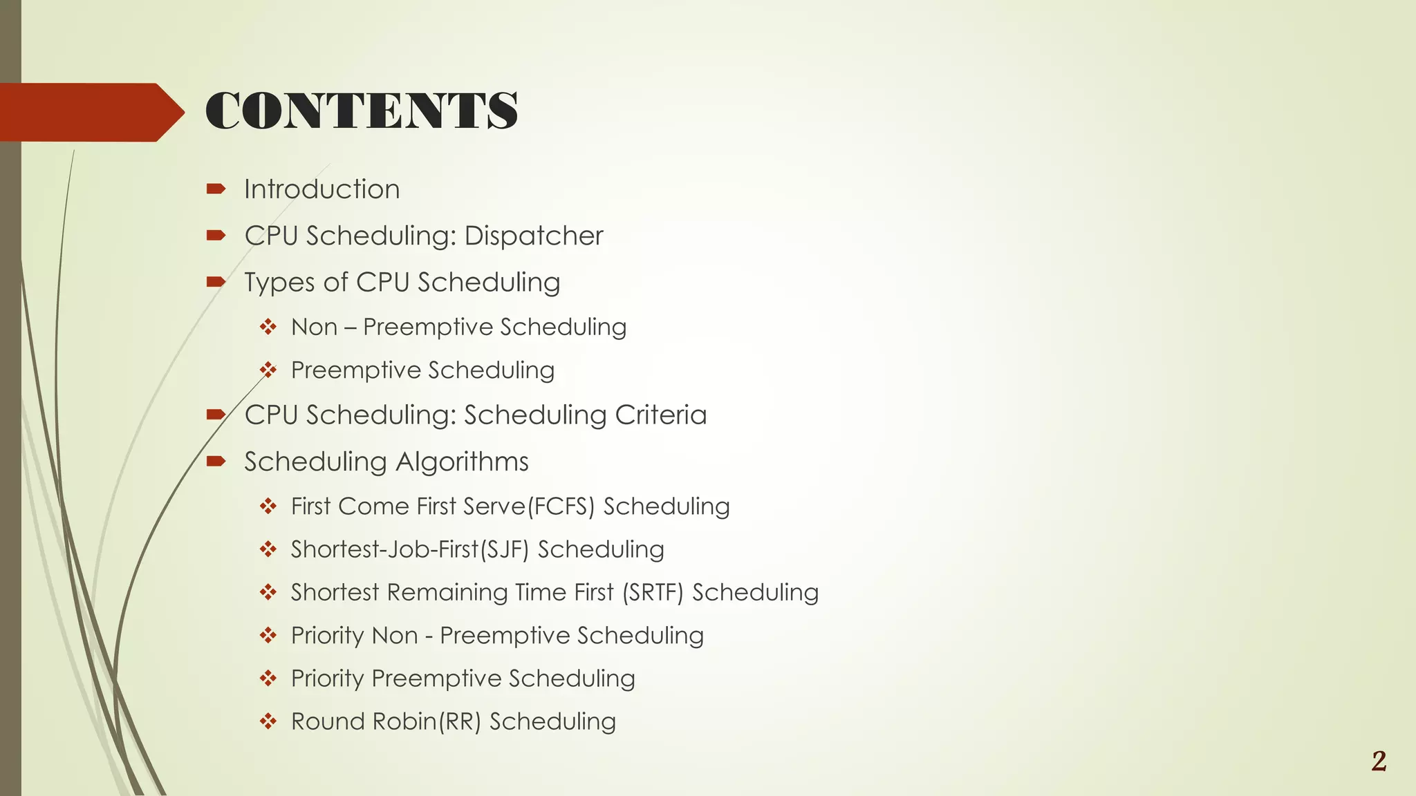
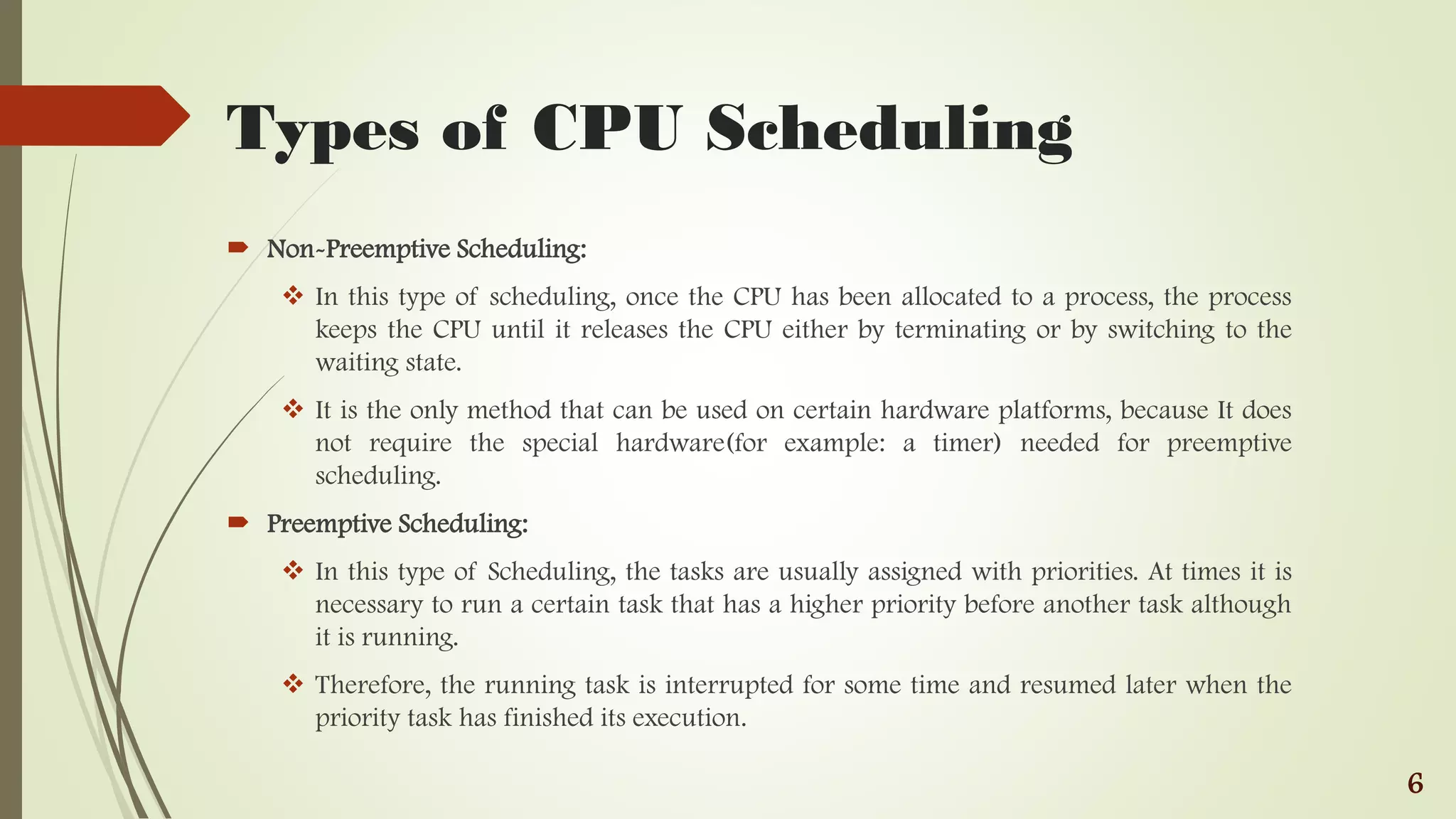
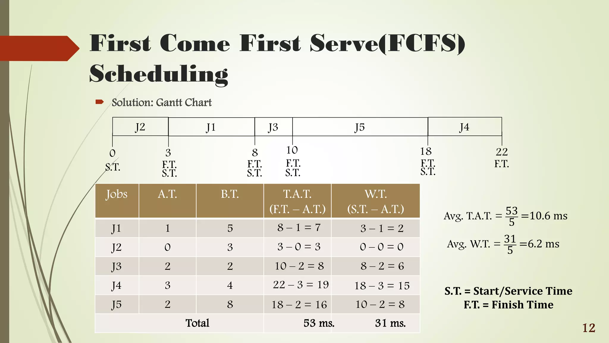
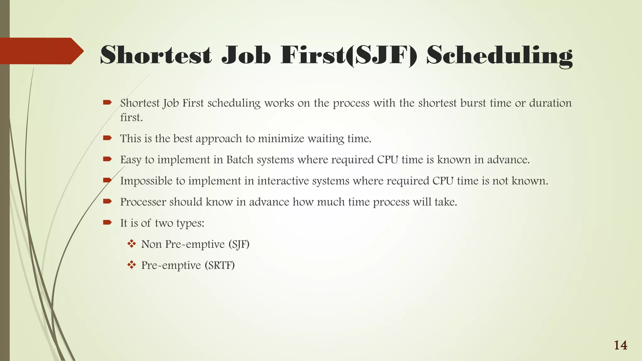
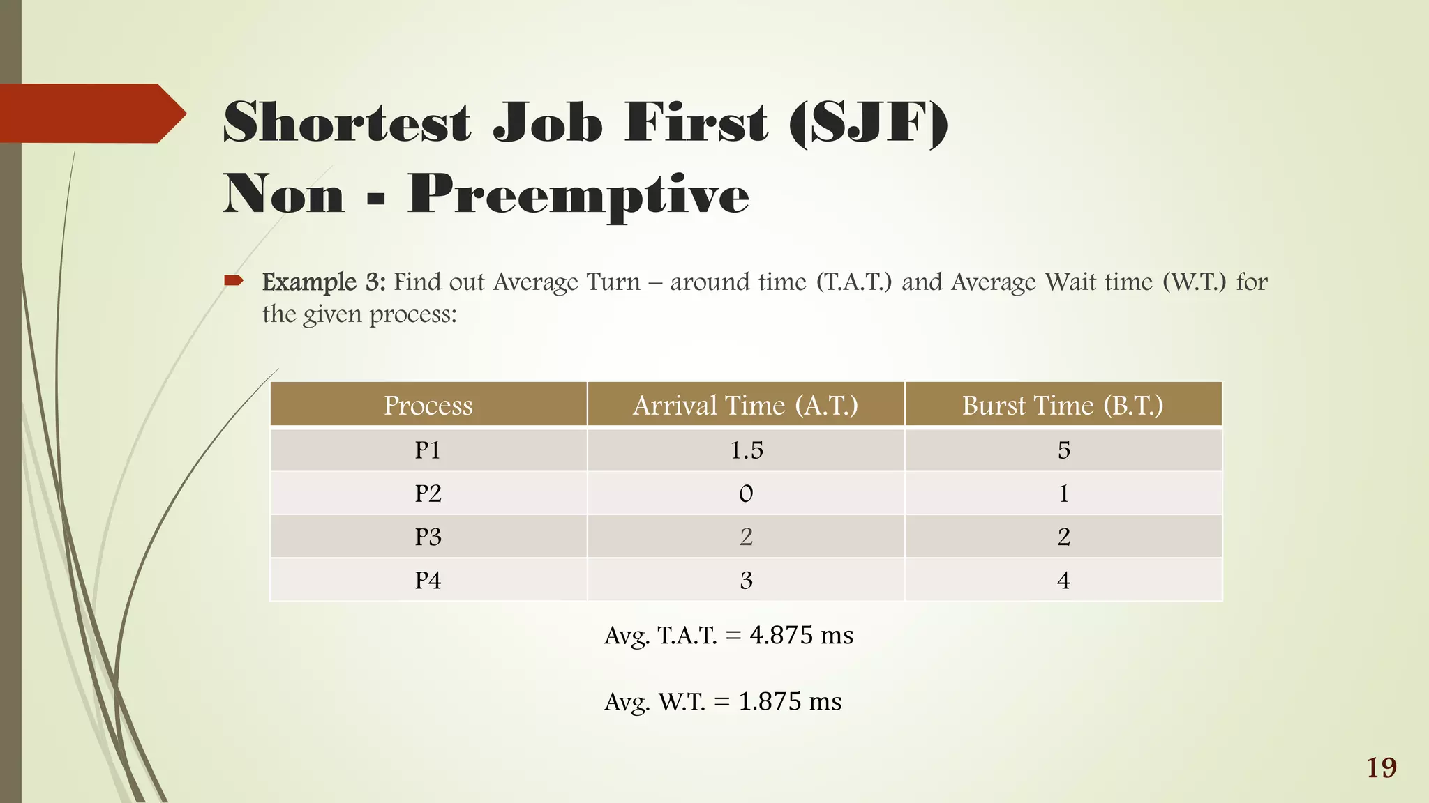
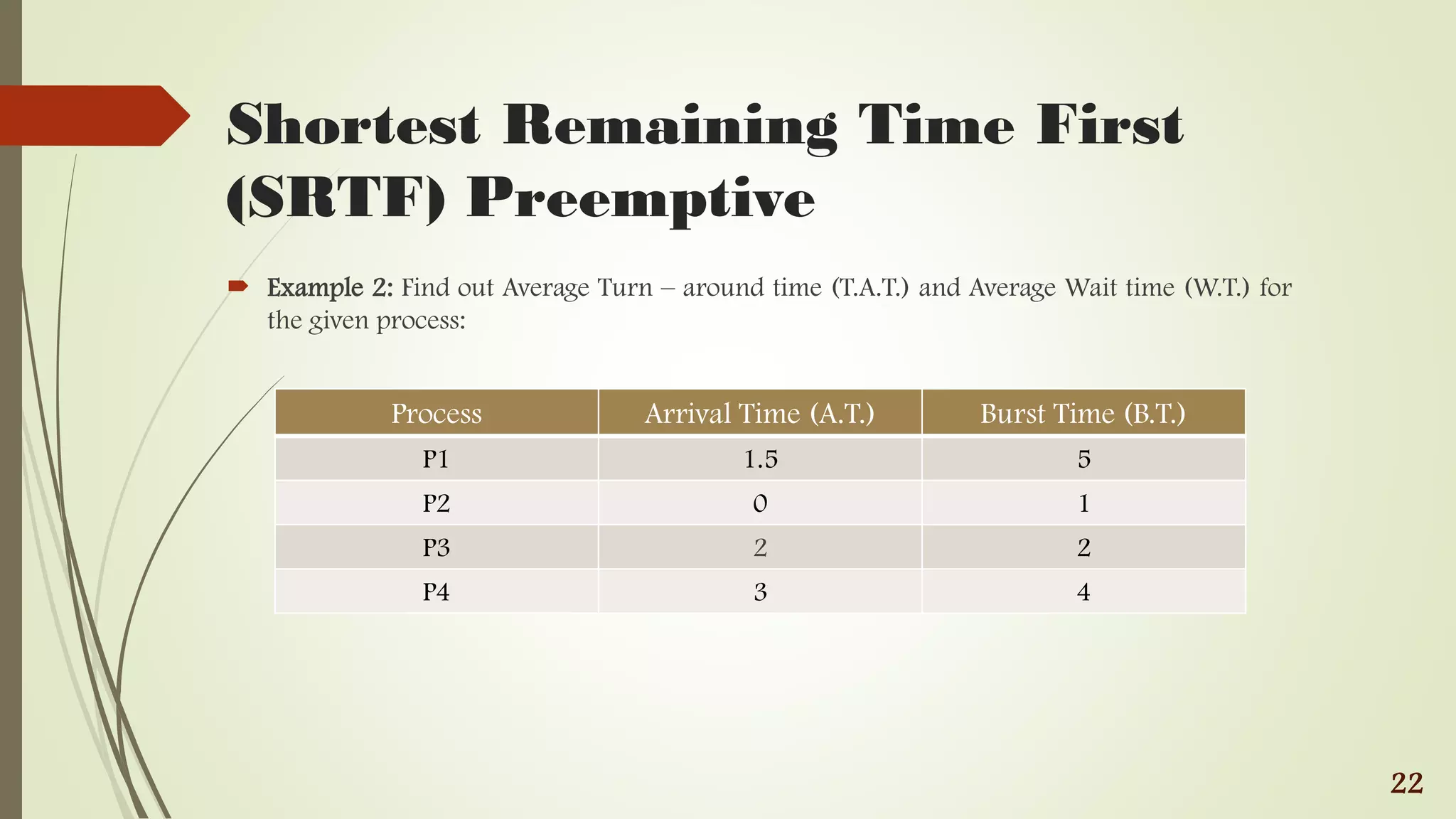
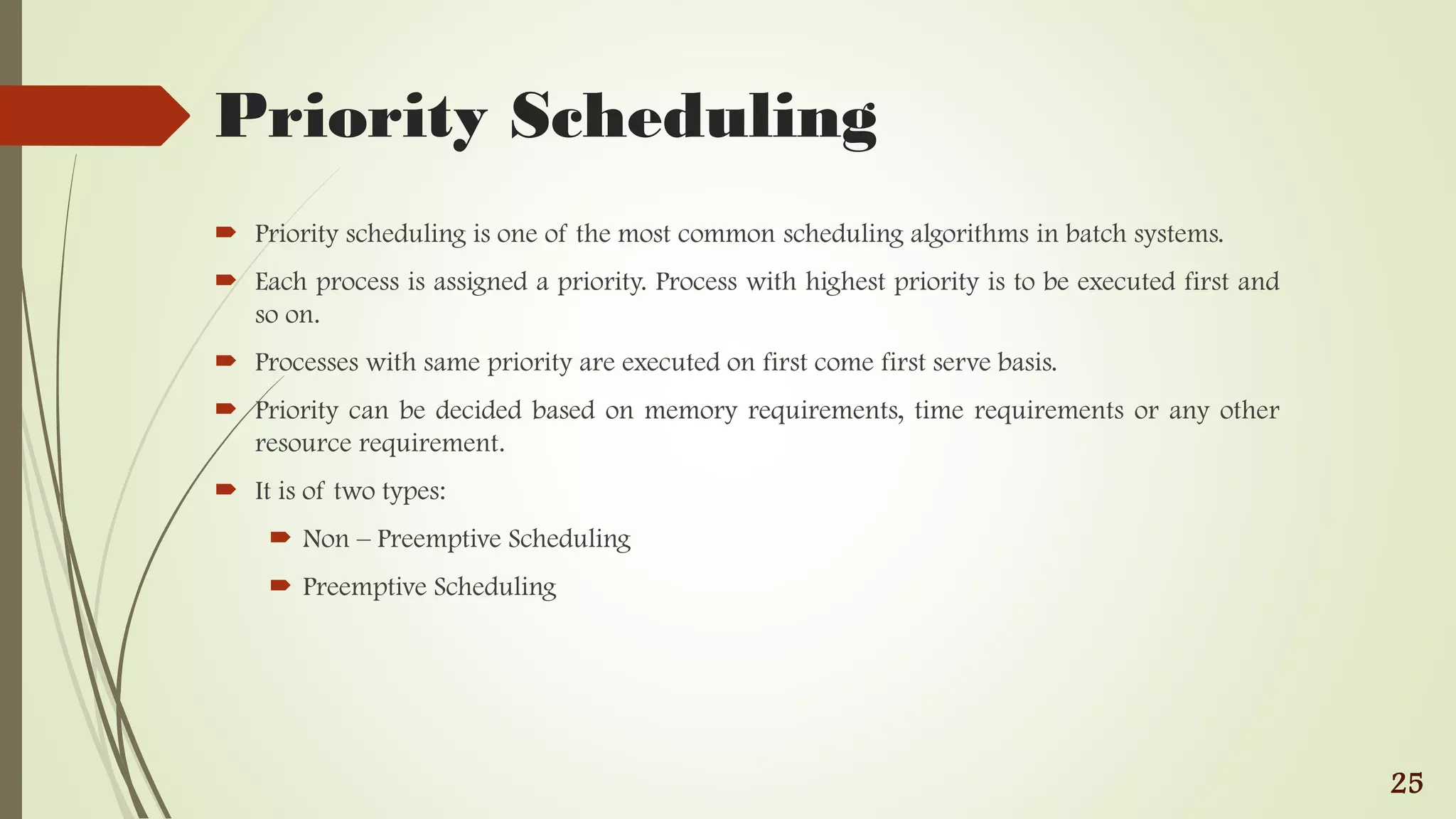
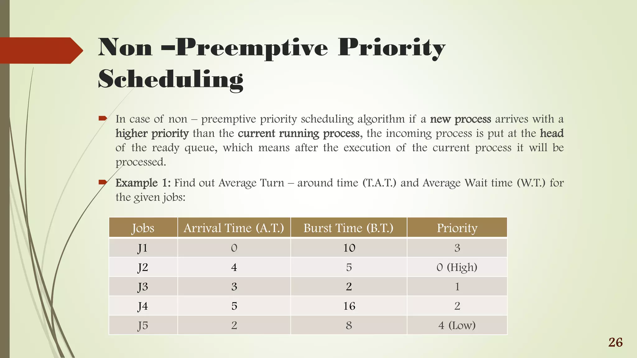
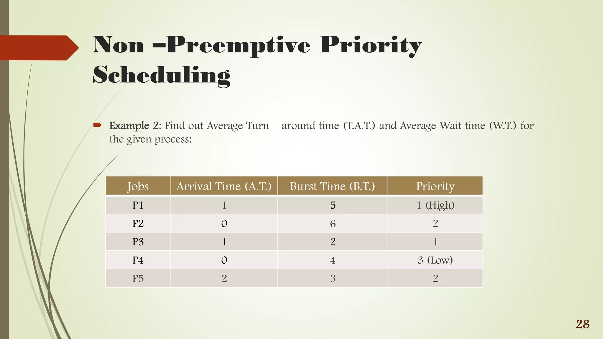
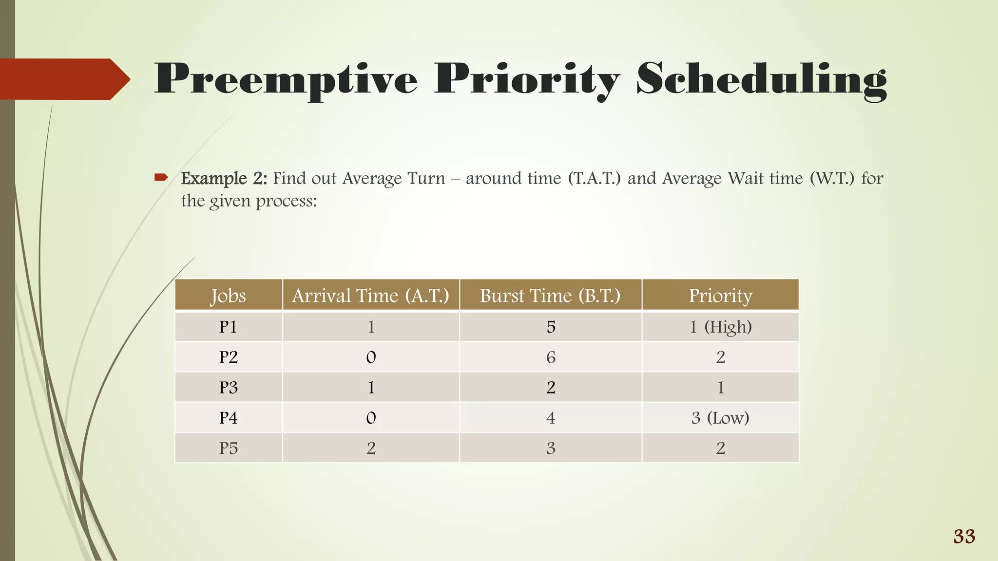
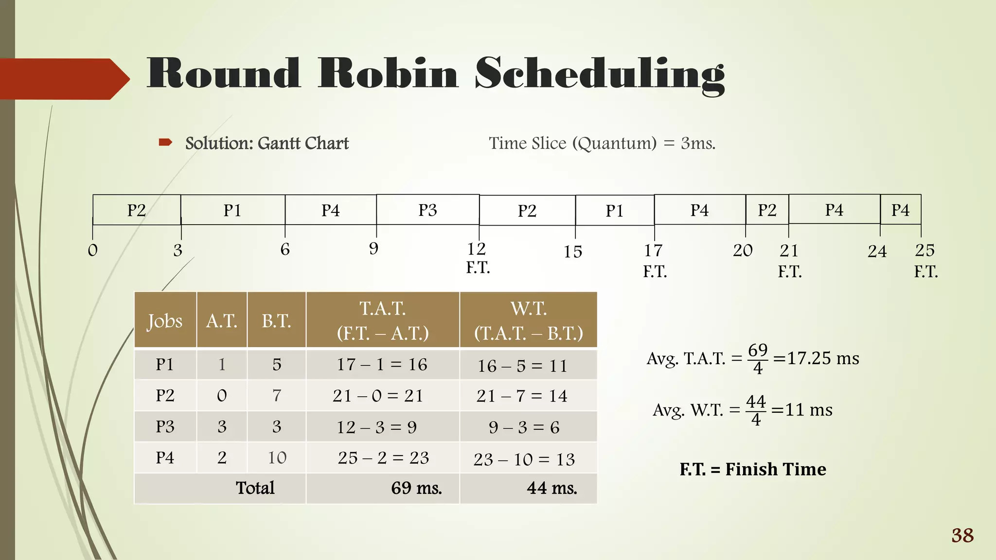
The document discusses CPU scheduling, which involves allocating CPU resources to processes in a way that maximizes efficiency, speed, and fairness. It categorizes CPU scheduling into non-preemptive and preemptive types, and details various scheduling algorithms such as First Come First Serve (FCFS), Shortest Job First (SJF), and priority scheduling. Additionally, it outlines scheduling criteria including CPU utilization, throughput, turnaround time, and waiting time, providing examples to demonstrate average turnaround and wait times.

1. CPU SCHEDULING
T.Y.B.Sc. (CS)
By: Ms. Farhat Rahat Ali Shaikh

2. CONTENTS
 Introduction
 CPU Scheduling: Dispatcher
 Types of CPU Scheduling
 Non – Preemptive Scheduling
 Preemptive Scheduling
 CPU Scheduling: Scheduling Criteria
 Scheduling Algorithms
 First Come First Serve(FCFS) Scheduling
 Shortest-Job-First(SJF) Scheduling
 Shortest Remaining Time First (SRTF) Scheduling
 Priority Non - Preemptive Scheduling
 Priority Preemptive Scheduling
 Round Robin(RR) Scheduling
2

3. Introduction
 CPU scheduling is a process which allows one process to use the CPU while the execution
of another process is on hold(in waiting state) due to unavailability of any resource like
I/O etc., thereby making full use of CPU. The aim of CPU scheduling is to make the
system efficient, fast and fair.
 Whenever the CPU becomes idle, the operating system must select one of the processes in
the ready queue to be executed. The selection process is carried out by the short-term
scheduler (or CPU scheduler). The scheduler selects from among the processes in
memory that are ready to execute, and allocates the CPU to one of them.
3

4. CPU Scheduling: Dispatcher
 The dispatcher is the module that gives control of the CPU to the process selected by the
short-term scheduler. This function involves:
 Switching context
 Switching to user mode
 Jumping to the proper location in the user program to restart that program from
where it left last time.
 The dispatcher should be as fast as possible, given that it is invoked during every process
switch. The time taken by the dispatcher to stop one process and start another process is
known as the Dispatch Latency.
4

5. Types of CPU Scheduling
 CPU scheduling decisions may take place under the following four circumstances:
 When a process switches from the running state to the waiting state (for I/O request or
invocation of wait for the termination of one of the child processes).
 When a process switches from the running state to the ready state (for example, when
an interrupt occurs).
 When a process switches from the waiting state to the ready state (for example,
completion of I/O).
 When a process terminates.
 In circumstances 1 and 4, there is no choice in terms of scheduling. A new process(if one
exists in the ready queue) must be selected for execution. There is a choice, however in
circumstances 2 and 3.
 When Scheduling takes place only under circumstances 1 and 4, we say the scheduling
scheme is Non-preemptive; otherwise the scheduling scheme is Preemptive.
5

6. Types of CPU Scheduling
 Non-Preemptive Scheduling:
 In this type of scheduling, once the CPU has been allocated to a process, the process
keeps the CPU until it releases the CPU either by terminating or by switching to the
waiting state.
 It is the only method that can be used on certain hardware platforms, because It does
not require the special hardware(for example: a timer) needed for preemptive
scheduling.
 Preemptive Scheduling:
 In this type of Scheduling, the tasks are usually assigned with priorities. At times it is
necessary to run a certain task that has a higher priority before another task although
it is running.
 Therefore, the running task is interrupted for some time and resumed later when the
priority task has finished its execution.
6

7. CPU Scheduling: Scheduling Criteria
 There are many different criteria's to check when considering the "best" scheduling
algorithm, they are:
 CPU Utilization: To make out the best use of CPU and not to waste any CPU cycle, CPU
would be working most of the time(Ideally 100% of the time). Considering a real
system, CPU usage should range from 40% (lightly loaded) to 90% (heavily loaded.)
 Throughput: It is the total number of processes completed per unit time or rather say
total amount of work done in a unit of time. This may range from 10/second to
1/hour depending on the specific processes.
 Turnaround Time: It is the amount of time taken to execute a particular process, i.e.
The interval from time of submission of the process to the time of completion of the
process(Wall clock time).
 Waiting Time: It is the total time spent by the process in the ready state waiting to get
control on the CPU.
7

8. CPU Scheduling: Scheduling Criteria
 Load Average: It is the average number of processes residing in the ready queue
waiting for their turn to get into the CPU.
 Response Time: Amount of time it takes from when a request was submitted until the
first response is produced. Remember, it is the time till the first response and not the
completion of process execution(final response).
 In general CPU utilization and Throughput are maximized and other factors are
reduced for proper optimization.
8

9. Scheduling Algorithms
 To decide which process to execute first and which process to execute last to achieve
maximum CPU utilization, we have various scheduling algorithms as follows :
 First Come First Serve(FCFS) Scheduling
 Shortest Job First(SJF) Scheduling
 Priority Scheduling
 Round Robin(RR) Scheduling
9

10. First Come First Serve(FCFS)
Scheduling
 In the "First come first serve" scheduling algorithm, the process which arrives first, gets
executed first, or we can say that the process which requests the CPU first, gets the CPU
allocated first.
 It is a Non-preemptive Scheduling algorithm.
 Easy to understand and implement.
 Its implementation is based on FIFO queue.
 Poor in performance as average wait time is high.
 This is used in Batch Systems.
10

11. First Come First Serve(FCFS)
Scheduling
 Example 1: Find out Average Turn – around time (T.A.T.) and Average Wait time (W.T.) for
the given jobs:
11
Jobs Arrival Time (A.T.) Burst Time (B.T.)
J1 1 5
J2 0 3
J3 2 2
J4 3 4
J5 2 8

12. First Come First Serve(FCFS)
Scheduling
 Solution: Gantt Chart
12
Jobs A.T. B.T. T.A.T.
(F.T. – A.T.)
W.T.
(S.T. – A.T.)
J1 1 5
J2 0 3
J3 2 2
J4 3 4
J5 2 8
J2
0 3
J1
8
J3
10
J5
18
J4
22
S.T. F.T.
8 – 1 = 7
3 – 0 = 3
10 – 2 = 8
22 – 3 = 19
18 – 2 = 16
S.T.
F.T.
S.T.
F.T.
S.T.
F.T.
S.T.
F.T.
3 – 1 = 2
0 – 0 = 0
8 – 2 = 6
18 – 3 = 15
10 – 2 = 8
Avg. T.A.T. = 53
5
=10.6 ms
Avg. W.T. = 31
5
=6.2 ms
Total 53 ms. 31 ms.
S.T. = Start/Service Time
F.T. = Finish Time

13. First Come First Serve(FCFS)
Scheduling
 Example 2: Find out Average Turn – around time (T.A.T.) and Average Wait time (W.T.) for
the given process:
13
Process Arrival Time (A.T.) Burst Time (B.T.)
P1 1 5
P2 0 6
P3 1 2
P4 0 4
Avg. T.A.T. = 11.5 ms
Avg. W.T. = 7.2 ms

14. Shortest Job First(SJF) Scheduling
 Shortest Job First scheduling works on the process with the shortest burst time or duration
first.
 This is the best approach to minimize waiting time.
 Easy to implement in Batch systems where required CPU time is known in advance.
 Impossible to implement in interactive systems where required CPU time is not known.
 Processer should know in advance how much time process will take.
 It is of two types:
 Non Pre-emptive (SJF)
 Pre-emptive (SRTF)
14

15. Shortest Job First (SJF)
Non - Preemptive
 In this type of scheduling CPU allocated to the process(min burst time) cannot be
preempted until completes its CPU burst.
 Example 1: Find out Average Turn – around time (T.A.T.) and Average Wait time (W.T.) for
the given jobs:
15
Jobs Arrival Time (A.T.) Burst Time (B.T.)
J1 0 4
J2 1 1
J3 2 2
J4 3 1

16. Shortest Job First (SJF)
Non - Preemptive
 Solution: Gantt Chart
16
Jobs A.T. B.T. T.A.T.
(F.T. – A.T.)
W.T.
(S.T. – A.T.)
J1 0 4
J2 1 1
J3 2 2
J4 3 1
J1
0 4
J2
5
J4
6
J3
8
S.T. F.T.
4 – 0 = 4
5 – 1 = 4
8 – 2 = 6
6 – 3 = 3
S.T.F.T. S.T.
F.T.
S.T.
F.T.
0 – 0 = 0
4 – 1 = 3
6 – 2 = 4
5 – 3 = 2
Avg. T.A.T. = 17
4
=4.2 ms
Avg. W.T. = 9
4
=2.2 ms
Total 17 ms. 9 ms.
S.T. = Start/Service Time
F.T. = Finish Time

17. Shortest Job First (SJF)
Non - Preemptive
 Example 2: Find out Average Turn – around time (T.A.T.) and Average Wait time (W.T.) for
the given process:
17
Jobs Arrival Time (A.T.) Burst Time (B.T.)
P1 3 5
P2 0 2
P3 4 2
P4 5 3

18. Shortest Job First (SJF)
Non - Preemptive
 Solution: Gantt Chart
18
Jobs A.T. B.T. T.A.T.
(F.T. – A.T.)
W.T.
(S.T. – A.T.)
P1 3 5
P2 0 2
P3 4 2
P4 5 3
P2
0 2
P1
14
P4
9
P3
6
S.T. F.T.
14 – 3 = 11
2 – 0 = 2
6 – 4 = 2
9 – 5 = 4
S.T.F.T. S.T.
F.T.S.T. F.T.
9 – 3 = 6
0 – 0 = 0
4 – 4 = 0
6 – 5 = 1
Avg. T.A.T. = 19
4
=4.75 ms
Avg. W.T. = 7
4
=1.75 ms
Total 19 ms. 7 ms.
S.T. = Start/Service Time
F.T. = Finish Time
4
Idle state

19. Shortest Job First (SJF)
Non - Preemptive
 Example 3: Find out Average Turn – around time (T.A.T.) and Average Wait time (W.T.) for
the given process:
19
Process Arrival Time (A.T.) Burst Time (B.T.)
P1 1.5 5
P2 0 1
P3 2 2
P4 3 4
Avg. T.A.T. = 4.875 ms
Avg. W.T. = 1.875 ms

20. Shortest Remaining Time First
(SRTF) Preemptive
 In Preemptive Shortest Job First Scheduling, jobs are put into ready queue as they arrive,
but as a process with short burst time arrives, the existing process is preempted or removed
from execution, and the shorter job is executed first.
 Example 1: Find out Average Turn – around time (T.A.T.) and Average Wait time (W.T.) for
the given jobs:
20
Jobs Arrival Time (A.T.) Burst Time (B.T.)
J1 0 4
J2 1 1
J3 2 2
J4 3 1

21. Shortest Remaining Time First
(SRTF) Preemptive
 Solution: Gantt Chart
21
Jobs A.T. B.T. T.A.T.
(F.T. – A.T.)
W.T.
(T.A.T. – B.T.)
J1 0 4
J2 1 1
J3 2 2
J4 3 1
J1
0 1
J2
2
J4
5
J3
4
8 – 0 = 8
2 – 1 = 1
4 – 2 = 2
5 – 3 = 2
F.T. F.T. F.T.
8 – 4 = 4
1 – 1 = 0
2 – 2 = 0
2 – 1 = 1
Avg. T.A.T. = 13
4
=3.25 ms
Avg. W.T. = 5
4
=1.25 ms
Total 13 ms. 5 ms.
F.T. = Finish Time
J3
3
J1
8
F.T.
CPU
J1 =
J2 =
J3 =
J4 =
3 =>
1 =>
2 =>
1 =>
0
1 => 0
0
0

22. Shortest Remaining Time First
(SRTF) Preemptive
 Example 2: Find out Average Turn – around time (T.A.T.) and Average Wait time (W.T.) for
the given process:
22
Process Arrival Time (A.T.) Burst Time (B.T.)
P1 1.5 5
P2 0 1
P3 2 2
P4 3 4

23. Shortest Remaining Time First
(SRTF) Preemptive
 Solution: Gantt Chart
23
Jobs A.T. B.T. T.A.T.
(F.T. – A.T.)
W.T.
(T.A.T. – B.T.)
P1 1.5 5
P2 0 1
P3 2 2
P4 3 4
P2
0 1 1.5
P3
4
P3
3
12.5 – 1.5 = 11
1 – 0 = 1
4 – 2 = 2
8 – 3 = 5
F.T. F.T. F.T.
11 – 5 = 6
1 – 1 = 0
2 – 2 = 0
5 – 4 = 1
Avg. T.A.T. = 19
4
=4.75 ms
Avg. W.T. = 7
4
=1.75 ms
Total 19 ms. 7 ms.
F.T. = Finish Time
P1
2
P4
8
F.T.
CPU
P2 =
P1 =
P3 =
P4 =
4.5 =>
0
2 =>
4 =>
0
1 => 0
0
Idle state
P1
12.5

24. Shortest Remaining Time First
(SRTF) Preemptive
 Example 3: Find out Average Turn – around time (T.A.T.) and Average Wait time (W.T.) for
the given process:
24
Jobs Arrival Time (A.T.) Burst Time (B.T.)
P1 3 5
P2 0 2
P3 4 2
P4 5 3
Avg. T.A.T. = 4.5 ms
Avg. W.T. = 1.5 ms

25. Priority Scheduling
 Priority scheduling is one of the most common scheduling algorithms in batch systems.
 Each process is assigned a priority. Process with highest priority is to be executed first and
so on.
 Processes with same priority are executed on first come first serve basis.
 Priority can be decided based on memory requirements, time requirements or any other
resource requirement.
 It is of two types:
 Non – Preemptive Scheduling
 Preemptive Scheduling
25

26. Non –Preemptive Priority
Scheduling
 In case of non – preemptive priority scheduling algorithm if a new process arrives with a
higher priority than the current running process, the incoming process is put at the head
of the ready queue, which means after the execution of the current process it will be
processed.
 Example 1: Find out Average Turn – around time (T.A.T.) and Average Wait time (W.T.) for
the given jobs:
26
Jobs Arrival Time (A.T.) Burst Time (B.T.) Priority
J1 0 10 3
J2 4 5 0 (High)
J3 3 2 1
J4 5 16 2
J5 2 8 4 (Low)

27. Non –Preemptive Priority
Scheduling
 Solution: Gantt Chart
27
Jobs A.T. B.T. Priority
T.A.T.
(F.T. – A.T.)
W.T.
(T.A.T. – B.T.)
J1 0 10 3
J2 4 5 0 (High)
J3 3 2 1
J4 5 16 2
J5 2 8 4 (Low)
J1
0 10
J2
15
J5
41
J4
33
10 – 0 = 10
15 – 4 = 11
17 – 3 = 14
33 – 5 = 28
F.T. F.T. F.T.
10 – 10 = 0
11 – 5 = 6
14 – 2 = 12
28 – 16 = 12
Avg. T.A.T. = 102
5
=20.4 ms
Avg. W.T. = 61
5
=12.2 ms
Total 102 ms. 61 ms.
F.T. = Finish Time
J3
17
F.T. F.T.
41 – 2 = 39 39 – 8 = 31

28. Non –Preemptive Priority
Scheduling
 Example 2: Find out Average Turn – around time (T.A.T.) and Average Wait time (W.T.) for
the given process:
28
Jobs Arrival Time (A.T.) Burst Time (B.T.) Priority
P1 1 5 1 (High)
P2 0 6 2
P3 1 2 1
P4 0 4 3 (Low)
P5 2 3 2

29. Non –Preemptive Priority
Scheduling
 Solution: Gantt Chart
29
Jobs A.T. B.T. Priority
T.A.T.
(F.T. – A.T.)
W.T.
(T.A.T. – B.T.)
P1 1 5 1 (High)
P2 0 6 2
P3 1 2 1
P4 0 4 3 (Low)
P5 2 3 2
P2
0 6
P1
11
P4
20
P5
16
11 – 1 = 10
6 – 0 = 6
13 – 1 = 12
20 – 0 = 20
F.T. F.T. F.T.
10 – 5 = 5
6 – 6 = 0
12 – 2 = 10
20 – 4 = 16
Avg. T.A.T. = 62
5
=12.4 ms
Avg. W.T. = 42
5
=8.4 ms
Total 62 ms. 42 ms.
F.T. = Finish Time
P3
13
F.T. F.T.
16 – 2 = 14 14 – 3 = 11

30. Non –Preemptive Priority
Scheduling
 Example 3: Find out Average Turn – around time (T.A.T.) and Average Wait time (W.T.) for
the given process:
30
Jobs Arrival Time (A.T.) Burst Time (B.T.) Priority
P1 0 4 3
P2 2 3 1(Low)
P3 1 7 4 (High)
P4 3 15 2
Avg. T.A.T. = 16 ms
Avg. W.T. = 8.75 ms

31. Preemptive Priority Scheduling
 If the new process arrived at the ready queue has a higher priority than the currently
running process, the CPU is preempted, which means the processing of the current process
is stopped and the incoming new process with higher priority gets the CPU for its
execution.
 Example 1: Find out Average Turn – around time (T.A.T.) and Average Wait time (W.T.) for
the given jobs:
31
Jobs Arrival Time (A.T.) Burst Time (B.T.) Priority
J1 0 10 3
J2 4 5 0 (High)
J3 3 2 1
J4 5 16 2
J5 2 8 4 (Low)

32. Preemptive Priority Scheduling
 Solution: Gantt Chart
32
Jobs A.T. B.T. Priority
T.A.T.
(F.T. – A.T.)
W.T.
(T.A.T. – B.T.)
J1 0 10 3
J2 4 5 0 (High)
J3 3 2 1
J4 5 16 2
J5 2 8 4 (Low)
J1
0 3
J1
33
J4
26
33 – 0 = 33
9 – 4 = 5
10 – 3 = 7
26 – 5 = 21
F.T. F.T. F.T.
33 – 10 = 23
5 – 5 = 0
7 – 2 = 5
21 – 16 = 5
Avg. T.A.T. = 105
5
=21 ms
Avg. W.T. = 61
5
=12.2 ms
Total 105 ms. 61 ms.
F.T. = Finish Time
J2
9
F.T. F.T.
41 – 2 = 39 39 – 8 = 31
J3
10
J5
41
J3
4

33. Preemptive Priority Scheduling
 Example 2: Find out Average Turn – around time (T.A.T.) and Average Wait time (W.T.) for
the given process:
33
Jobs Arrival Time (A.T.) Burst Time (B.T.) Priority
P1 1 5 1 (High)
P2 0 6 2
P3 1 2 1
P4 0 4 3 (Low)
P5 2 3 2

34. Preemptive Priority Scheduling
 Solution: Gantt Chart
34
Jobs A.T. B.T. Priority
T.A.T.
(F.T. – A.T.)
W.T.
(T.A.T. – B.T.)
P1 1 5 1 (High)
P2 0 6 2
P3 1 2 1
P4 0 4 3 (Low)
P5 2 3 2
P2
0 1
P1
6
P4
20
P5
16
11 – 1 = 10
6 – 0 = 6
13 – 1 = 12
20 – 0 = 20
F.T.F.T. F.T.
10 – 5 = 5
6 – 6 = 0
12 – 2 = 10
20 – 4 = 16
Avg. T.A.T. = 62
5
=12.4 ms
Avg. W.T. = 42
5
=8.4 ms
Total 62 ms. 42 ms.
F.T. = Finish Time
P3
8
F.T. F.T.
16 – 2 = 14 14 – 3 = 11
P2
13

35. Preemptive Priority Scheduling
 Example 3: Find out Average Turn – around time (T.A.T.) and Average Wait time (W.T.) for
the given process:
35
Jobs Arrival Time (A.T.) Burst Time (B.T.) Priority
P1 0 4 3
P2 2 3 1(Low)
P3 1 7 4 (High)
P4 3 15 2
Avg. T.A.T. = 17 ms
Avg. W.T. = 9.75 ms

36. Round Robin Scheduling
 Round Robin is the preemptive process scheduling algorithm.
 Each process is provided a fix time to execute called quantum.
 Once a process is executed for given time period. Process is preempted and other process
executes for given time period.
 Context switching is used to save states of preempted processes.
36

37. Round Robin Scheduling
 Example 1: Find out Average Turn – around time (T.A.T.) and Average Wait time (W.T.) for
the given process with Time Slice (Quantum) = 3ms.
37
Jobs Arrival Time (A.T.) Burst Time (B.T.)
P1 1 5
P2 0 7
P3 3 3
P4 2 10

38. Round Robin Scheduling
 Solution: Gantt Chart Time Slice (Quantum) = 3ms.
38
Jobs A.T. B.T.
T.A.T.
(F.T. – A.T.)
W.T.
(T.A.T. – B.T.)
P1 1 5
P2 0 7
P3 3 3
P4 2 10
P2
0 3
P1
6
P1
17
P2
15
17 – 1 = 16
21 – 0 = 21
12 – 3 = 9
25 – 2 = 23
F.T.F.T. F.T.
16 – 5 = 11
21 – 7 = 14
9 – 3 = 6
23 – 10 = 13
Avg. T.A.T. = 69
4
=17.25 ms
Avg. W.T. = 44
4
=11 ms
Total 69 ms. 44 ms.
F.T. = Finish Time
P4
9
F.T.
P3
12
P4
20
P2
21
P4
24
P4
25

39. Round Robin Scheduling
 Example 2: Find out Average Turn – around time (T.A.T.) and Average Wait time (W.T.) for
the given process with Time Slice (Quantum) = 2ms.
39
Jobs Arrival Time (A.T.) Burst Time (B.T.)
P1 1 5
P2 0 3
P3 2 2
P4 3 4
P5 13 2

40. Round Robin Scheduling
40
Jobs A.T. B.T.
T.A.T.
(F.T. – A.T.)
W.T.
(T.A.T. – B.T.)
P1 1 5
P2 0 3
P3 2 2
P4 3 4
P5 13 2
P2
0 2
P1
4
P1
11
P2
9
16 – 1 = 15
9 – 0 = 9
6 – 2 = 4
13 – 3 = 10
F.T.F.T.F.T.
15 – 5 = 10
9 – 3 = 6
4 – 2 = 2
10 – 4 = 6
Avg. T.A.T. = 40
5
=8 ms
Avg. W.T. = 24
5
=4.8 ms
Total 40 ms. 24 ms.
F.T. = Finish Time
P3
6
F.T.
P4
8
P4
13
P5
15
P1
16
 Solution: Gantt Chart Time Slice (Quantum) = 2ms.
F.T.
15 – 13 = 2 2 – 2 = 0

41. Round Robin Scheduling
 Example 2: Five jobs arrive at 0 arrival time the order is given below. Find out Average
Turn – around time (T.A.T.) and Average Wait time (W.T.) for the given process with
Time Slice (Quantum) = 10ms.
41
Jobs Burst Time (B.T.)
J1 10
J2 29
J3 3
J4 7
J5 12
Avg. T.A.T. = 35.2 ms
Avg. W.T. = 23 ms

42. THANK YOU
42