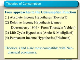
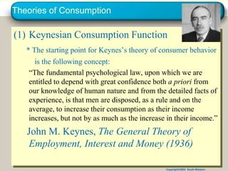
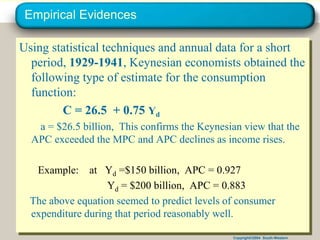
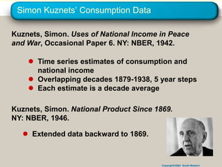
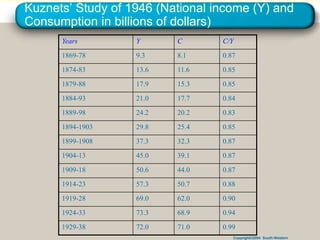
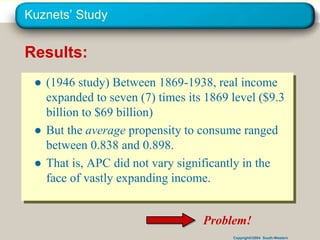
consumption function macro economics.ppt

Copyright©2004 South-Western 1 of 36
A Shocking Rise in White Death Rates in Midlife—and What It Says
about American Society by Anne Case and Angus Deaton

Copyright©2004 South-Western
The Structure of the Model
I—The Spending Sector
* Consumption, Investment, Government and Net exports
II—The Monetary Sector
* Money demand and Money Supply
* Financial sector
III—The Production Sector
*Capital, Labor…..
IV—The Labor Market Sector
*Labor Demand and Supply

Consumption Function
● A good illustration of the interplay of theory and data.
● The consumption/saving decision is the key behavioral
element of the Solow growth model.
● Also underlies the multiplier effects in the short run
model.
● Consumption is also the biggest component of AD.
● We cannot have a good understanding of the economy
unless we have a good theory of consumption
● The primary motivation of the chapter is the puzzle of
the difference between the short-run (cross-section)
and long-run (time-series) consumption function.

U.S. consumption, 2014:2
(RGDP=$15,994.3 chained 2009)
44.9
14.71
8.8
68.23%
7180.4
2,352.9
1,401.0
$10,910.4
Services
Nondurables
Durables
Consumption
% of GDP
Chained $
billions

U.S. Investment, 2014:2
0.5
3.1
13.1
16.9%
83.9
493.8
2,093.3
$2,694.7
Inventory
Residential
Business fixed
Investment
% of GDP
Chained $
billions

● Share of consumers spending

● Each blue dot represents
consumption expenditure and
disposable income in the United
States for a year between 1960
and 2007.
The U.S. Consumption Function
The line CF0 is an estimate
of the U.S. consumption
function during the 1960s.
The line CF1 is an estimate of
the U.S. consumption
function during the 2000s.

● The slope of the consumption
function—the marginal propensity
to consume—is 0.87.
The U.S. Consumption Function
The consumption function
shifted upward as influences
on consumption expenditure
other than disposable income
changed.

Figure 9.2 (a) Growth in Consumption and Investment
Mankiw: Macroeconomics, Seventh Edition
Copyright © 2010 by Worth Publishers

U.S. Personal Saving

Theories of Consumption
Four approaches to the Consumption Function
(1) Absolute Income Hypotheses (Keynes?)
(2) Relative Income Hypothesis (James
Duesenberry 1949 ~ From Thorstein Veblen)
(3) Life Cycle Hypothesis (Ando & Modigliani)
(4) Permanent Income Hypothesis (Friedman)
Theories 3 and 4 are most compatible with Neo-
classical economics.

Theories of Consumption
(1) Keynesian Consumption Function
* The starting point for Keynes’s theory of consumer behavior
is the following concept:
“The fundamental psychological law, upon which we are
entitled to depend with great confidence both a priori from
our knowledge of human nature and from the detailed facts of
experience, is that men are disposed, as a rule and on the
average, to increase their consumption as their income
increases, but not by as much as the increase in their income.”
John M. Keynes, The General Theory of
Employment, Interest and Money (1936)

(1) Keynesian Consumption Function
• This psychological law translates into the Keynesian consumption
function:
C = a + b*Yd Where a > 0, 0 < b < 1
b = Marginal Propensity to consume (MPC) =ΔC/ΔYd
APC = Average Propensity to consume = C/Yd
APC = a/Yd + b
This implies APC is greater than MPC and follows that the
APC declines as the level of income increases.
This version of the consumption function (specifically when
a =0, C = b*Yd ) has been called the Absolute Income
Hypothesis; consumption is assumed to react rather
mechanically to actual current levels of income.

Keynes’s Conjectures
Keynes’s simple consumption function can
be summarized:
(a) Current consumption depends on
current income.
(b)The MPC is between zero and one.
(c) The APC is a decreasing function of
income.

The Keynesian Consumption Function
slope = APC
As income rises, the APC falls (consumers
save a bigger fraction of their income).
C = a + b*Yd
C
Y d

Implications:
The fact that the proportion of income saved apparently
increased as income rose led some early Keynesians to
be concerned about secular stagnation in the economy.
The Stagnation thesis (Alvin Hansen, 1939)
* Due to lack of effective demand. (unless balanced by
the growth of the other components aggregate demand:
government spending & Investment.

Empirical Evidences
Using statistical techniques and annual data for a short
period, 1929-1941, Keynesian economists obtained the
following type of estimate for the consumption
function:
C = 26.5 + 0.75 Yd
a = $26.5 billion, This confirms the Keynesian view that the
APC exceeded the MPC and APC declines as income rises.
Example: at Yd =$150 billion, APC = 0.927
Yd = $200 billion, APC = 0.883
The above equation seemed to predict levels of consumer
expenditure during that period reasonably well.

Empirical Evidences…
Further support for the Keynesian form of the
consumption function came from comparative
studies of families budgets.
*Looking at budgets for families at progressively higher
income levels, the absolute amount of consumption
increased (MPC > 0), But by less than the increase in
income ( 0 < MPC < 1)
* Families at a higher income levels consumed a smaller
proportion of income.  APC declined as income rose.

Simon Kuznets’ Consumption Data
Kuznets, Simon. Uses of National Income in Peace
and War, Occasional Paper 6. NY: NBER, 1942.
 Time series estimates of consumption and
national income
 Overlapping decades 1879-1938, 5 year steps
 Each estimate is a decade average
Kuznets, Simon. National Product Since 1869.
NY: NBER, 1946.
 Extended data backward to 1869.

Kuznets’ Study of 1946 (National income (Y) and
Consumption in billions of dollars)
Years Y C C/Y
1869-78 9.3 8.1 0.87
1874-83 13.6 11.6 0.85
1879-88 17.9 15.3 0.85
1884-93 21.0 17.7 0.84
1889-98 24.2 20.2 0.83
1894-1903 29.8 25.4 0.85
1899-1908 37.3 32.3 0.87
1904-13 45.0 39.1 0.87
1909-18 50.6 44.0 0.87
1914-23 57.3 50.7 0.88
1919-28 69.0 62.0 0.90
1924-33 73.3 68.9 0.94
1929-38 72.0 71.0 0.99

Kuznets’ Study
● (1946 study) Between 1869-1938, real income
expanded to seven (7) times its 1869 level ($9.3
billion to $69 billion)
● But the average propensity to consume ranged
between 0.838 and 0.898.
● That is, APC did not vary significantly in the
face of vastly expanding income.
Results:
Problem!

Empirical Evidences…
● Consumption and National Income (1869-1938)
by Simon Kuznets
* There was no downward trend in the ratio real
consumption to real national income.
* Nor is there evidence for a downward trend in APC
in more recent years.
Example: 1950 APC=0.93
1970 APC=0.89
1990 APC=0.93

Resolving the Empirical Puzzles
● Evidences from short-run annual time series
data (1929-41) and family budget studies
seemed to support the Keynesian view
● Times series data for a longer time period
(1969-1938) suggest that the consumption-
income relationship is proportional rather than
the non-proportional relationship given by
absolute income hypothesis.
● Resolving these puzzles has been the task of the
modern theory of the consumption function.

The Consumption Puzzle
C
Y
Consumption function
from long time series
data (constant APC )
Consumption function
from cross-sectional
household data
(falling APC )

Reconciliation with Keynes’ Theory?
t = 1923
t = 1924
t = 1925
Kuznets
Yt*
Ct*
 Arthur Smithies,
Econometrica, 1954.
 Uses per capita Yd and C,
and a time trend.
 Argues that the Cons.
Function is really Keynesian,
but just looks Kuznets’
because of the shifts in the
function.
 Says the data points just
“happen” to line up to fit
Kuznets’ consumption
function.

Second Failure of Keynesian Consumption
Function
● Predictions of post-WWII period are grossly wrong
● Keynesian Theory argues that the average propensity
to save (APS) rises with income (S = S0 + sY).
● Higher post-war incomes should imply excess saving.
Will we go straight back to the Depression?
● Comparison of the forecasts with the actual results
suggest that:
■ consumption was “under”-predicted
■ saving was “over”-predicted
● IMPLICATION: major determinants in the behavioral
equations must be missing!

(2) The Relative Income Hypothesis
James Duesenberry’s approach says that people are not
just concerned about absolute levels of possession.
They are in fact concerned about their possessions
relative to others, “Keeping up with the Jones.”
● People are not necessarily happier if they have more
money. They do however report higher happiness if
they have more relative to others.
Current economists still support this idea. Ex: Robert
Frank
● Duesenberry argues that we have a greater tendency to
resist spending decreases relative to falls in income
than we do to increase expenditure relative to increases
of income. The reason is that we don’t want to alter
our standard of living downward. Duesenberry’s
Habit Persistence Theory

Irving Fisher and Intertemporal Choice (1930)
● The consumption function by Keynes does not
consider how people make decisions over time.
In other words, when people decide how much
to consume and how much to save, they take
into account both the present and the future.
● People face a tradeoff
● Fisher developed an intertemporal model that
shows how households make decisions about
how much to consume and how much to save.

Intertemporal Budget Constraint
● Let us consider an individual who gets income
today and tomorrow and who consumes today
and tomorrow. What is her budget constraint?
In the first period, she gets income Y1, which
she consumes C1 or saves S:
Y1 = C1 + S.
In the second period, she earns interest on her
savings. Her consumption in the 2nd period:
C2 = Y2 + S (1 + r)

Intertemporal Budget Constraint….
● From the first equation
Y1 - C1 = S.
Substituting into the second equation, we
obtain:
C1 (1+r) + C2 = Y1(1+r) + Y2
Or
C1 + C2/(1+r)= Y1 + Y2 /(1+r)
The present value of consumption must equal the
present value of income. It is the consumer’s
intertemporal budget constraint.

The Intertemporal Budget Constraint
c1
c2
y2
y1
0
0
is the consumption bundle
when period 1 borrowing
is as big as possible.
is the consumption bundle when
period 1 saving is as large as possible.
r
y
y


1
2
1
1
2 )
1
( Y
r
Y 


Life Cycle Hypothesis (LCH)
● Franco Modigliani, Albert Ando, and Richard
Bloomberg (1954) proposed an explanation based
on the ideas in the Fisher model.
● They focused on the role of saving in smoothing
individuals’ consumption over their lifetimes.
“ The point of departure of the life cycle model is the hypothesis that
consumption and saving decisions of households at each point of
time reflect a more or less conscious attempt at achieving the
preferred distribution of consumption over the life cycle, subject
to the constraint imposed by the resources accruing to the
household over its lifetime.”
Franco Madigliani

Income and Consumption—LCH
death
T
Consumption
Income
Dissaving
Saving

Life Cycle….
● A stylized fact of economic data is that
consumption is much smoother than income.
● Let us consider the budget constraint of
someone who expects to live for T more
years, of which R will be spent working and
T-R will spent in retirement with zero
earnings.
● The consumer smoothes consumption
expenditure over his/her life, spending 1/T of
his/her life-time income each period.

Income and Consumption—LCH
● Assuming the initial wealth, W, and the real
interest rate is zero, the constraint will be:
C1 + C2 +…+ CT = W + Y1 + Y2 +…+ YR
CT = W + RY
C = (W + RY)/T
Example: consumer expects to live for 60 years
and working for 40 years. The function is
C = 0.017 W + 0.67Y
Therefore Consumption depends on both income
and wealth.

Testing the LCH
● If the function form looks like this:
● Ando and Modigliani argue that expected future labor
income is proportional to current income, so that the
function can be reduced to:
● When they estimate this function, they get:
t
e
t
t A
b
Y
b
Y
b
C 3
2
1 


t
t
t A
b
Y
b
b
C 3
2
1 )
( 

 
t
t
t A
Y
C 06
.
0
72
.
0 


● The ratio of labor income to disposable income
is 0.88 and the ratio of wealth to disposable
income is 4.75. That means A=4.75Y
● this leads to
)
75
.
4
(
06
.
0
)
88
(.
72
.
0 d
d
t Y
Y
C 

d
t Y
C 92
.
0


Policy Implications of LCH
● Changes in current income have a strong effect on
current consumption ONLY if they affect expected
lifetime income.
● In Q2 1975, a one-time tax rebate of $8 billion was
paid out to taxpayers to stimulate AD.
■ The rebate had little effect.
The only way there can be a significant effect is if
there is a strong liquidity constraint operating.
● This has implications for monetary policy.

Criticisms of LCH
● The households, at all times, have a definite,
conscious vision of:
■ The family’s future size and composition, including
the life expectancy of each member,
■ The entire lifetime profile of the labor income of
each member—after the applicable taxes,
■ The present and future extent and terms of any
credit available, and
■ The future emergencies, opportunities, and social
pressures which might affect its consumption
spending.
● It does not take into account liquidity constraints.

Permanent Income Hypothesis (PIH)
● Milton Friedman (A Theory of the Consumption Function. Princeton
Univ. Press, 1957)
● Assumptions:
■ Perfect certainty about:
♦ Future receipts
♦ Future interest rates
♦ Future prices, etc.
■ People save to reduce fluctuations in expenditures
■ People are immortal (or leave bequests)
● Individual’s utility function:
u = u(c,c1)
where c is current period consumption and c1 is next period consumption.
● People maximize utility based on their permanent (expected
life-time) income
● Allocate their income inter-temporally

PIH
● Friedman postulates that consumption is proportional to
permanent income:
k = factor of proportionality (k>0)
● Friedman does not expect the above consumption function
to predict consumption perfectly. Because measured
income (Y) contains a random element called transitory
income:
p
t
t kY
C 
p
t
Y
Y
Y 


(4) The Permanent Income Hypothesis
Suggested by Milton Friedman (1957)
• This hypothesis shares with the life cycle the assumption that long-term income is the
primary determinant of consumption.
● Milton Friedman argues that it would be more sensible for people to use current
income, but also at the same time to form expectations about future levels of income
and the relative amounts of risk.
● Thus, they are forming an analysis of “permanent income.”
Permanent Income = Past Income + Expected Future Income
● Transitory Income – Income that is earned in excess of, or perceived as an unexpected
windfall. If you get income not equal to what you expected or to what you don’t expect
to get again.
● So, he argues that we tend to spend more out of permanent income than out of
transitory.
● In the Friedman analysis, he treats people as forming their level of expected future
income based on their past incomes. This is known as adaptive expectations.
● Adaptive Expectations – looking forward in time using past expectations. In this case,
we use a distributed lag of past income.

Reviews on the modern theory
●The lifecycle hypotheses pays more attention to
the motives for saving,and provides convincing
reasons to include wealth as well as income in the
C function.
●The permanent income hypotheses pays more
attention to the way in which individuals form
expectations about their future income.
●Modern form of the consumption equation
C = a Wealth + b YD + c YD-1

Consumption
● The following are the five most important
variables that determine the level of consumption:
■ Current disposable income
■ Household wealth
■ Expected future income
■ The price level
■ The interest rate

consumption function macro economics.ppt

More Related Content

Similar to consumption function macro economics.ppt

More from SubhanAli78

Recently uploaded

consumption function macro economics.ppt