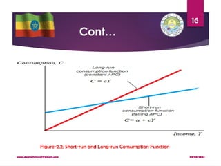
The document discusses the Keynesian consumption function, which posits that consumer spending is primarily determined by current real disposable income, emphasizing concepts like marginal propensity to consume (MPC) and average propensity to consume (APC). It details the empirical validation of Keynes' theories and introduces the notion of short-run versus long-run consumption functions, suggesting that while Keynes' model holds in the short run, it does not fully explain consumption patterns over the long term. Additionally, various hypotheses, including Fisher’s intertemporal model, are reviewed to explain consumer behavior and the consumption puzzle.


![08/08/2024
www.dagimfetene7@gmail.com
20
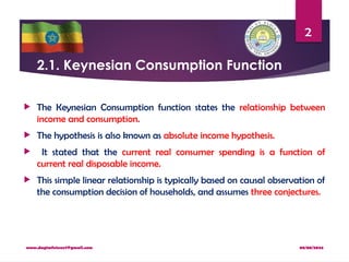
2.3.1. Keynesian absolute income hypothesis
Keynes proposed that consumption is a function of absolute level of
income [C= f(Y)].
In other words, the consumption function can be stated as; C = a + cY.
Where c is the marginal propensity to consume (which is the percentage
change in consumption due to change in income).
Income is the most important explanatory variable of consumption; but
interest rate is irrelevant in explaining consumption.
Some economists argued that interest rate determines consumption level.
When interest rate in the banks increases, people save more money in
banks to receive the higher interest income and consume less.](https://image.slidesharecdn.com/macroiichapter2-240808093539-4821ef34/85/Macro-II-Chapter-2-pptx-For-economics-stude-20-320.jpg)


![08/08/2024
www.dagimfetene7@gmail.com
59
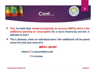
Cont…
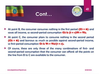
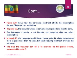
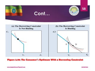
The analysis of borrowing constraints leads us to conclude that there are
two consumption functions.
For some consumers, the borrowing constraint is not binding, and
consumption in both periods depends on the present value of lifetime
income, Y1 + [Y2/(1 + r)].
For other consumers, the borrowing constraint binds, and the
consumption function is C1 = Y1 and C2 = Y2.
Hence, for those consumers who would like to borrow but cannot,
consumption depends only on current income.](https://image.slidesharecdn.com/macroiichapter2-240808093539-4821ef34/85/Macro-II-Chapter-2-pptx-For-economics-stude-59-320.jpg)