UNIT III MESSAGEROUTING
TECHNOLOGIES
Circuit switching, packet switching, message
switching. Internet protocols; IPV4, IPV6, ARP,
RARP, ICMP, IGMP, VPN. Network Routing
Algorithms:- Distance vector routing, OSPF,
Dijikstra‘s , Bellaman Ford, Congestion control
algorithms
2.
Network Layer
•The Networklayer is responsible for
the source-to-destination delivery of a
packet possible across multiple
networks.
• It converts Frames into packets.
Switching
• A networkis a set of connected devices(Whenever we
have multiple devices, we have the problem of how to
connect them to make one-to-one communication
possible)
• One solution is to make a point-to-point connection
between each pair of devices (a mesh topology) or
between a central device and every other device (a star
topology).
• These methods, however, are impractical and wasteful
when applied to very large networks.
• The number and length of the links require too much
infrastructure to be cost-efficient, and the majority of
those links would be idle most of the time.
A better solution is SWITCHING
6.
Switching
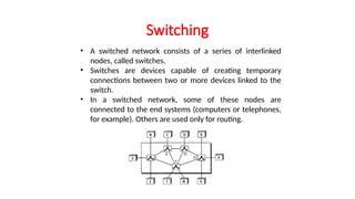
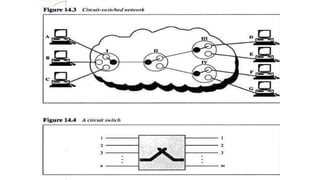
• A switchednetwork consists of a series of interlinked
nodes, called switches.
• Switches are devices capable of creating temporary
connections between two or more devices linked to the
switch.
• In a switched network, some of these nodes are
connected to the end systems (computers or telephones,
for example). Others are used only for routing.
7.
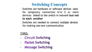
Switching Concepts
Switches arehardware or software devices used
for temporary connection b/w 2 or more
devices linked to the switch in network but not
to each another
Switches are needed to connect multiple devices
for making one-one communication
TYPES:
•
•
•
9.
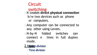
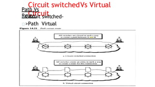
Circuit
switching
It creates directphysical connection
b/w two devices such as phone
or computers.
Any computer can be connected to
any other using Levers.
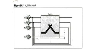
N-by-N folded switches can
connect n lines in full duplex
mode.
2 types:
◦
12.
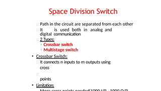
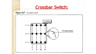
Space Division Switch
Pathin the circuit are separated from each other
It is used both in analog and
digital communication
2 Types:
◦ Crossbar switch
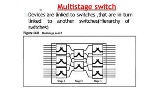
◦ Multistage switch
• Crossbar Switch:
It connects n inputs to m outputs using
cross
points
• Limitation:
Blocking:
The reduction ina number of cross
points causes a phenomena called
Blocking.
During heavy traffic one input
cannot be connected to output
because no path available
16.
Time Division Switches
Ituses time division multiplexing
2 methods:
Time slot
interchange TDM
bus
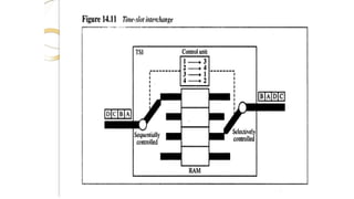
Time slot
interchange:
It changesthe ordering of the slot based on
the desired connection
It uses RAM to store time
slot Ex:
1->3 2->4 3->1 4-
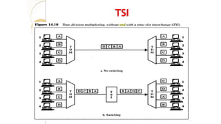
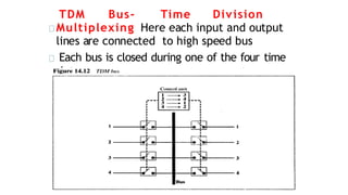
TDM Bus- TimeDivision
Multiplexing Here each input and output
lines are connected to high speed bus
Each bus is closed during one of the four time
slots
20.
Limitations of Circuit
Switching
•It is specially designed for
voice suitabl
e
communication(telephone).
Not for data communication.
• Once a circuit is
established, it remains
for
duration of the session. It
creates
dialed(temporary)and
leased(Permanent).
• Less data rate because of point
to connection.
poin
t
21.
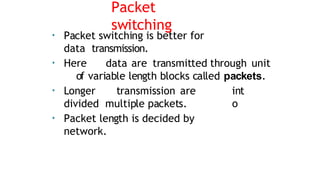
Packet
switching
• Packet switchingis better for
data transmission.
• Here data are transmitted through unit
of variable length blocks called packets.
• Longer transmission are
divided multiple packets.
• Packet length is decided by
network.
int
o
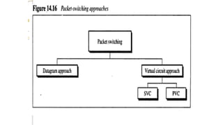
23.
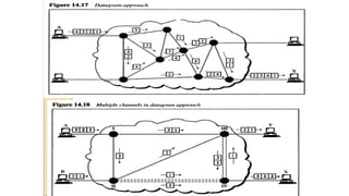
Datagram Approach
• Inthis approach a message is divided
into multiple packets.
• All packets choose various routes
and reaches the destination.
• Ordering of packets in destination is done
by transport layer
.
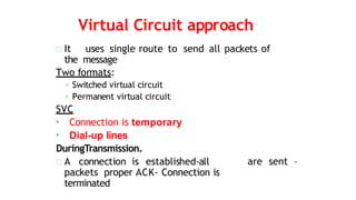
Virtual Circuit approach
Ituses single route to send all packets of
the message
Two formats:
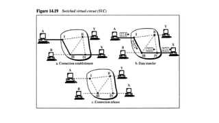
◦ Switched virtual circuit
◦ Permanent virtual circuit
SVC
• Connection is temporary
• Dial-up lines
DuringTransmission.
A connection is established-all
packets proper ACK- Connection is
terminated
are sent –
27.
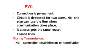
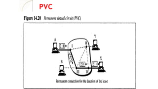
PVC
• Connection ispermanent.
• Circuit is dedicated for two users, No one
else can use the line when
communication takes place.
• It always gets the same route.
• Leased lines.
During Transmission.
No connection establishment or termination
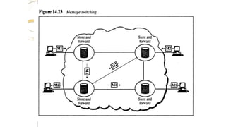
Message
Switching
• It usesa mechanism called store and
forward
• Here a message is received and stored
until a appropriate route is free, then
sends along.
• Message switching- uses
secondary storage(Disk)
• Packet switching – uses
primary storage(RAM)
32.
20.32
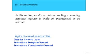
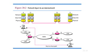
20-1 INTERNETWORKING
In thissection, we discuss internetworking, connecting
networks together to make an internetwork or an
internet.
Need for Network Layer
Internet as a Datagram Network
Internet as a Connectionless Network
Topics discussed in this section:
20.39
20-2 IPv4
The InternetProtocol version 4 (IPv4) is the delivery
mechanism used by the TCP/IP protocols.
Datagram
Fragmentation
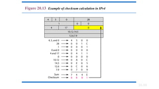
Checksum
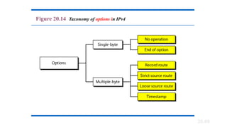
Options
Topics discussed in this section:
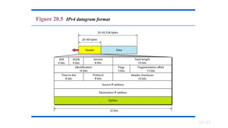
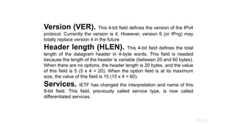
Version (VER). This4-bit field defines the version of the IPv4
protocol. Currently the version is 4. However, version 6 (or IPng) may
totally replace version 4 in the future
Header length (HLEN). This 4-bit field defines the total
length of the datagram header in 4-byte words. This field is needed
because the length of the header is variable (between 20 and 60 bytes).
When there are no options, the header length is 20 bytes, and the value
of this field is 5 (5 x 4 = 20). When the option field is at its maximum
size, the value of this field is 15 (15 x 4 = 60).
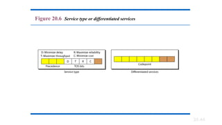
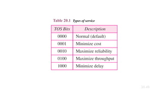
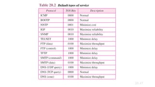
Services. IETF has changed the interpretation and name of this
8-bit field. This field, previously called service type, is now called
differentiated services.
20.42
43.
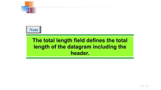
· Total Length---Specifiesthe length, in bytes, of the entire IP packet.
· Identification---Contains an integer that identifies the current datagram.
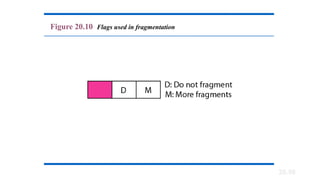
· Flags---The two low-order (least-significant) bits control fragmentation. The low-order bit
specifies whether the packet can be fragmented. The middle bit specifies whether the
packet is the last fragment in a series of fragmented packets. The third or high-order bit is
not used.
· Fragment Offset---Indicates the position of the fragment's data relative to the beginning of
the data in the original datagram.
· Time-to-Live---Maintains a counter that gradually decrements down to zero, at which point
the datagram is discarded. This keeps packets from looping endlessly.
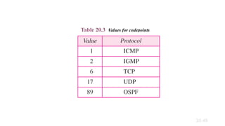
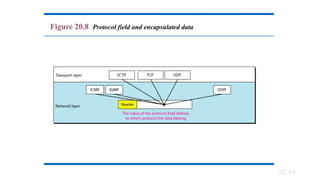
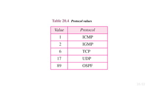
· Protocol---Indicates which upper-layer protocol receives incoming packets after IP processing
is complete.
· Header Checksum---Helps ensure IP header integrity.
· Source Address---Specifies the sending node.
· Destination Address---Specifies the receiving node.
· Options---Allows IP to support various options, such as security.
· Data---Contains upper-layer information.
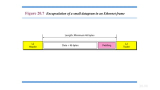
20.53
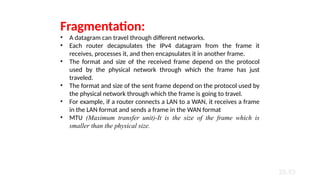
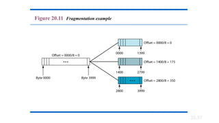
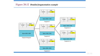
Fragmentation:
• A datagramcan travel through different networks.
• Each router decapsulates the IPv4 datagram from the frame it
receives, processes it, and then encapsulates it in another frame.
• The format and size of the received frame depend on the protocol
used by the physical network through which the frame has just
traveled.
• The format and size of the sent frame depend on the protocol used by
the physical network through which the frame is going to travel.
• For example, if a router connects a LAN to a WAN, it receives a frame
in the LAN format and sends a frame in the WAN format
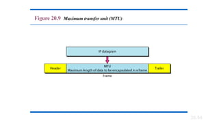
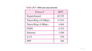
• MTU (Maximum transfer unit)-It is the size of the frame which is
smaller than the physical size.
20.61
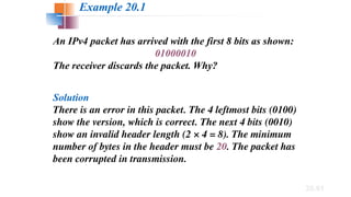
An IPv4 packethas arrived with the first 8 bits as shown:
01000010
The receiver discards the packet. Why?
Solution
There is an error in this packet. The 4 leftmost bits (0100)
show the version, which is correct. The next 4 bits (0010)
show an invalid header length (2 × 4 = 8). The minimum
number of bytes in the header must be 20. The packet has
been corrupted in transmission.
Example 20.1
62.
20.62
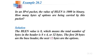
In an IPv4packet, the value of HLEN is 1000 in binary.
How many bytes of options are being carried by this
packet?
Solution
The HLEN value is 8, which means the total number of
bytes in the header is 8 × 4, or 32 bytes. The first 20 bytes
are the base header, the next 12 bytes are the options.
Example 20.2
63.
20.63
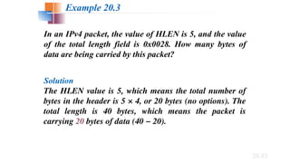
In an IPv4packet, the value of HLEN is 5, and the value
of the total length field is 0x0028. How many bytes of
data are being carried by this packet?
Solution
The HLEN value is 5, which means the total number of
bytes in the header is 5 × 4, or 20 bytes (no options). The
total length is 40 bytes, which means the packet is
carrying 20 bytes of data (40 − 20).
Example 20.3
64.
20.64
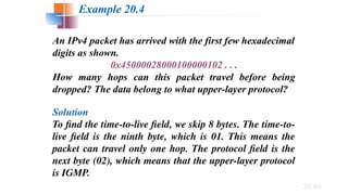
An IPv4 packethas arrived with the first few hexadecimal
digits as shown.
0x45000028000100000102 . . .
How many hops can this packet travel before being
dropped? The data belong to what upper-layer protocol?
Solution
To find the time-to-live field, we skip 8 bytes. The time-to-
live field is the ninth byte, which is 01. This means the
packet can travel only one hop. The protocol field is the
next byte (02), which means that the upper-layer protocol
is IGMP.
Example 20.4
65.
19-1 IPv4ADDRESSES
An IPv4address is a 32-bit address that uniquely and
universally defines the connection of a device (for
example, a computer or a router) to the Internet.
Topics discussed in this section:
Address Space
Notations
Classful Addressing
Classless
Addressing
Network Address
Translation (NAT)
19.
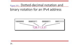
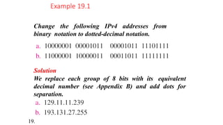
Change the followingIPv4 addresses from
binary notation to dotted-decimal notation.
Example 19.1
Solution
We replace each group of 8 bits with its equivalent
decimal number (see Appendix B) and add dots for
separation.
19.
72.
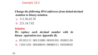
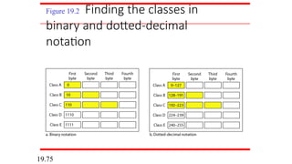
Change the followingIPv4 addresses from dotted-decimal
notation to binary notation.
Example 19.2
Solution
We replace each decimal number with its
binary equivalent (see Appendix B).
19.
73.
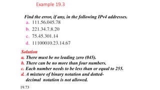
Find the error,if any, in the following IPv4 addresses.
Example 19.3
Solution
a. There must be no leading zero (045).
b. There can be no more than four numbers.
c. Each number needs to be less than or equal to 255.
d. A mixture of binary notation and dotted-
decimal notation is not allowed.
19.73
74.
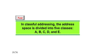
In classful addressing,the address
space is divided into five classes:
A, B, C, D, and E.
Note
19.74
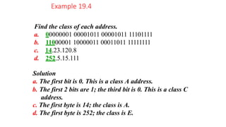
Find the classof each address.
a. 00000001 00001011 00001011 11101111
b. 11000001 10000011 00011011 11111111
c. 14.23.120.8
d. 252.5.15.111
Solution
a. The first bit is 0. This is a class A address.
b. The first 2 bits are 1; the third bit is 0. This is a class C
address.
c. The first byte is 14; the class is A.
d. The first byte is 252; the class is E.
Example 19.4
77.
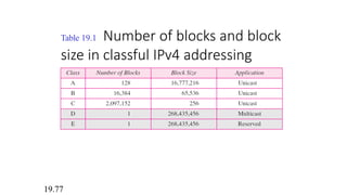
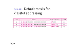
Table 19.1 Numberof blocks and block
size in classful IPv4 addressing
19.77
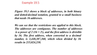
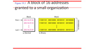
Figure 19.3 showsa block of addresses, in both binary
and dotted-decimal notation, granted to a small business
that needs 16 addresses.
We can see that the restrictions are applied to this block.
The addresses are contiguous. The number of addresses
is a power of 2 (16 = 24), and the first address is divisible
by 16. The first address, when converted to a decimal
number, is 3,440,387,360, which when divided by 16
results in 215,024,210.
Example 19.5
82.
Figure 19.3 Ablock of 16 addresses
granted to a small organization
83.
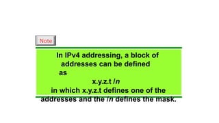
In IPv4 addressing,a block of
addresses can be defined
as
x.y.z.t /n
in which x.y.z.t defines one of the
addresses and the /n defines the mask.
Note
84.
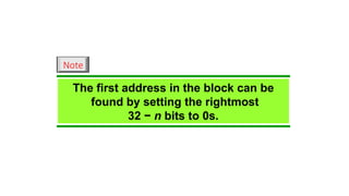
The first addressin the block can be
found by setting the rightmost
32 − n bits to 0s.
Note
85.
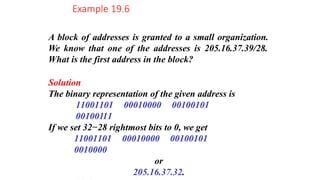
A block ofaddresses is granted to a small organization.
We know that one of the addresses is 205.16.37.39/28.
What is the first address in the block?
Solution
The binary representation of the given address is
11001101 00010000 00100101
00100111
If we set 32−28 rightmost bits to 0, we get
11001101 00010000 00100101
0010000
or
205.16.37.32.
Example 19.6
86.
The last addressin the block can be
found by setting the rightmost
32 − n bits to 1s.
Note
87.
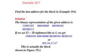
Find the lastaddress for the block in Example 19.6.
Solution
The binary representation of the given address is
11001101 00010000 00100101
00100111
If we set 32 − 28 rightmost bits to 1, we get
11001101 00010000 00100101 00101111
or
205.16.37.47
This is actually the block
shown in Figure 19.3.
Example 19.7
88.
The number ofaddresses in the block
can be found by using the formula
232−n.
Note
89.
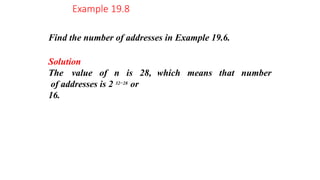
Find the numberof addresses in Example 19.6.
Example 19.8
Solution
The value of n is 28,
of addresses is 2 32−28
or
16.
which means that number
90.
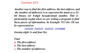
Another way tofind the first address, the last address, and
the number of addresses is to represent the mask as a 32-
bit binary (or 8-digit hexadecimal) number. This is
particularly useful when we are writing a program to find
these pieces of information. In Example 19.5 the /28 can
be represented as
11111111 11111111 11111111 11110000
(twenty-eight 1s and four 0s).
Find
a. The first address
b. The last address
c. The number of addresses.
Example 19.9
91.
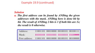
Solution
a. The firstaddress can be found by ANDing the given
addresses with the mask. ANDing here is done bit by
bit. The result of ANDing 2 bits is 1 if both bits are 1s;
the result is 0 otherwise.
Example 19.9 (continued)
92.
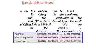
b. The lastaddress can be found
by ORing the given addresses
with the complement of the
mask. ORing here is done bit by bit. The result
of ORing 2 bits is 0 if both bits are
0s; the result is 1
otherwise. The complement of a
number is found by changing each 1
to 0 and each 0 to 1.
Example 19.9 (continued)
93.
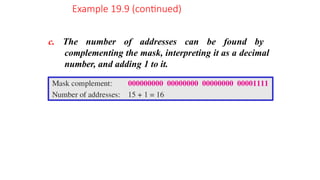
c. The numberof addresses can be found by
complementing the mask, interpreting it as a decimal
number, and adding 1 to it.
Example 19.9 (continued)
94.
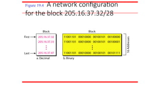
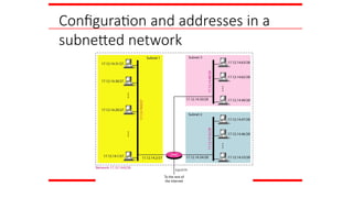
Figure 19.4 Anetwork configuration
for the block 205.16.37.32/28
95.
The first addressin a block is
normally not assigned to any device;
it is used as the network address that
represents the organization
to the rest of the world.
Note
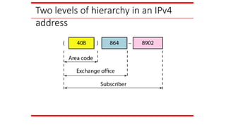
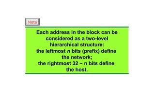
Each address inthe block can be
considered as a two-level
hierarchical structure:
the leftmost n bits (prefix) define
the network;
the rightmost 32 − n bits define
the host.
Note
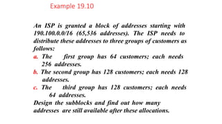
An ISP isgranted a block of addresses starting with
190.100.0.0/16 (65,536 addresses). The ISP needs to
distribute these addresses to three groups of customers as
follows:
a. The first group has 64 customers; each needs
256 addresses.
b. The second group has 128 customers; each needs 128
addresses.
c. The third group has 128 customers; each needs
64 addresses.
Design the subblocks and find out how many
addresses are still available after these allocations.
Example 19.10
102.
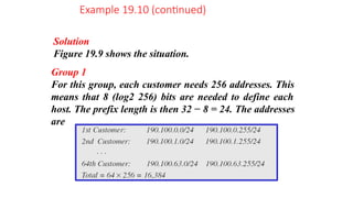
Solution
Figure 19.9 showsthe situation.
Group 1
For this group, each customer needs 256 addresses. This
means that 8 (log2 256) bits are needed to define each
host. The prefix length is then 32 − 8 = 24. The addresses
are
Example 19.10 (continued)
103.
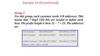
Example 19.10 (continued)
Group2
For this group, each customer needs 128 addresses. This
means that 7 (log2 128) bits are needed to define each
host. The prefix length is then 32 − 7 = 25. The addresses
are
104.
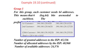
Example 19.10 (continued)
Group3
For this group, each customer needs 64 addresses.
This means that 6 (log264) bits areneeded to
eachhost. The
prefix length is then 32 − 6 = 26. The addresses are
Number of granted addresses to the ISP: 65,536
Number of allocated addresses by the ISP: 40,960
Number of available addresses: 24,576
105.
The network layerprotocol in the TCP/IP protocol suite
is currently IPv4. Although IPv4 is well designed, data
communication has evolved since the inception of IPv4
in the 1970s. IPv4 has some deficiencies that make it
unsuitable for the fast-growing Internet.
Advantages
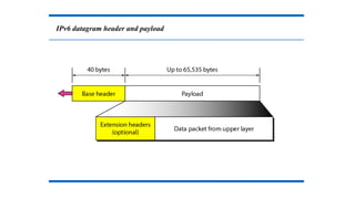
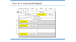
Packet Format
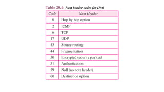
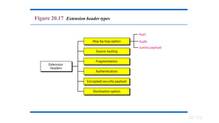
Extension Headers
Topics discussed in this section:
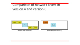
IPv6
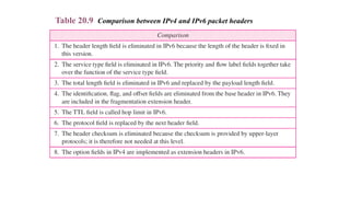
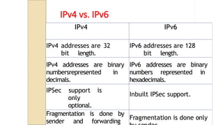
IPv4 vs. IPv6
IPv4IPv6
IPv4 addresses are 32
bit length.
IPv6 addresses are 128
bit length.
IPv4 addresses are binary
numbersrepresented in
decimals.
IPv6 addresses are binary
numbers represented in
hexadecimals.
IPSec support is
only
optional.
Inbuilt IPSec support.
Fragmentation is done by
sender and forwarding
Fragmentation is done only
115.
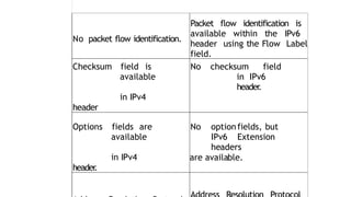
No packet flowidentification.
Packet flow identification is
available within the IPv6
header using the Flow Label
field.
Checksum field is
available
in IPv4
header
No checksum field
in IPv6
header
.
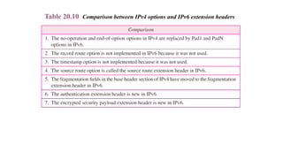
Options fields are
available
in IPv4
header
.
No optionfields, but
IPv6 Extension
headers
are available.
116.
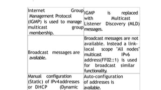
Internet Group
Management Protocol
(IGMP)is used to manage
multicast group
membership.
IGMP is replaced
with Multicast
Listener Discovery (MLD)
messages.
Broadcast messages are
available.
Broadcast messages are not
available. Instead a link-
local scope "All nodes"
multicast IPv6
address(FF02::1) is used
for broadcast similar
functionality.
Manual configuration
(Static) of IPv4addresses
or DHCP (Dynamic
Auto-configuration
of addresses is
available.
117.
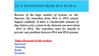
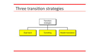
20-4 TRANSITION FROMIPv4 TO IPv6
Because of the huge number of systems on the
Internet, the transition from IPv4 to IPv6 cannot
happen suddenly. It takes a considerable amount of
time before every system in the Internet can move from
IPv4 to IPv6. The transition must be smooth to
prevent any problems between IPv4 and IPv6 systems.
Topics discussed in this section:
Dual Stack
Tunneling
Header
Translatio
118.
•Complete transition fromIPv4 to IPv6 might
not be possible because IPv6 is not backward
compatible.
•This results in a situation where either a site is
on IPv6 or it is not.
•It is unlike implementation of other new
technologies where the newer one is backward
compatible so the older system can still work
with the newer version without any additional
changes.
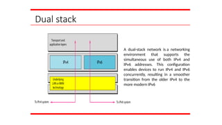
Dual stack
A dual-stacknetwork is a networking
environment that supports the
simultaneous use of both IPv4 and
IPv6 addresses. This configuration
enables devices to run IPv4 and IPv6
concurrently, resulting in a smoother
transition from the older IPv4 to the
more modern IPv6
121.
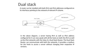
A router canbe installed with both IPv4 and IPv6 addresses configured on
its interfaces pointing to the network of relevant IP scheme.
Dual stack
In the above diagram, a server having IPv4 as well as IPv6 address
configured for it can now speak with all the hosts on both the IPv4 as well
as the IPv6 networks with the help of a Dual Stack Router. The Dual Stack
Router, can communicate with both the networks. It provides a medium
for the hosts to access a server without changing their respective IP
versions.
122.
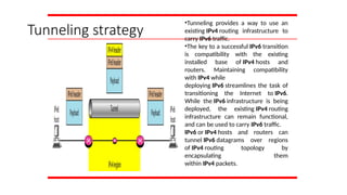
Tunneling strategy
•Tunneling providesa way to use an
existing IPv4 routing infrastructure to
carry IPv6 traffic.
•The key to a successful IPv6 transition
is compatibility with the existing
installed base of IPv4 hosts and
routers. Maintaining compatibility
with IPv4 while
deploying IPv6 streamlines the task of
transitioning the Internet to IPv6.
While the IPv6 infrastructure is being
deployed, the existing IPv4 routing
infrastructure can remain functional,
and can be used to carry IPv6 traffic.
IPv6 or IPv4 hosts and routers can
tunnel IPv6 datagrams over regions
of IPv4 routing topology by
encapsulating them
within IPv4 packets.
123.
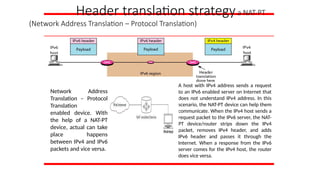
Header translation strategyaNAT-PT
(Network Address Translation – Protocol Translation)
Network Address
Translation – Protocol
Translation
enabled device. With
the help of a NAT-PT
device, actual can take
place happens
between IPv4 and IPv6
packets and vice versa.
A host with IPv4 address sends a request
to an IPv6 enabled server on Internet that
does not understand IPv4 address. In this
scenario, the NAT-PT device can help them
communicate. When the IPv4 host sends a
request packet to the IPv6 server, the NAT-
PT device/router strips down the IPv4
packet, removes IPv4 header, and adds
IPv6 header and passes it through the
Internet. When a response from the IPv6
server comes for the IPv4 host, the router
does vice versa.
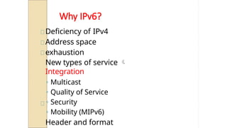
Why IPv6?
Deficiency ofIPv4
Address space
exhaustion
New types of service
Integration
◦ Multicast
◦ Quality of Service
◦ Security
◦ Mobility (MIPv6)
Header and format
126.
Advantages of IPv6over IPv4
Larger address
space Better
header format
New options
Allowance for extension
Support for resource
allocation Support for more
security Support for
mobility
127.
IPv4 companion protocols(1)
ARP: Address Resolution Protocol
◦ Mapping from IP address to MAC address
ICMP: Internet Control Message
Protocol
◦ Error reporting & Query
IGMP: Internet Group Management
Protocol
◦ Multicast member join/leave
Unicast Routing Protocols (Intra-AS)
◦ Maintaining Unicast Routing Table
◦ E.g. RIP, OSPF (Open Shortest Path
128.
IPv4 companion protocols(2)
Multicast Routing Protocols
◦ Maintaining Multicast Routing Table
◦ E.g. DVMRP, MOSPF, CBT, PIM
Exterior Routing Protocols (Inter-
AS)
◦ E.g. BGP (Border Gateway Protocol)
Quality-of-Service Frameworks
◦ Integrated Service (ISA, IntServ)
◦ Differentiated Service (DiffServ)
129.
21-1 ADDRESS MAPPING
Thedelivery of a packet to a host or a router requires
two levels of addressing: logical and physical. We need
to be able to map a logical address to its corresponding
physical address and vice versa. This can be done by
using either static or dynamic mapping.
Topics discussed in this section:
Mapping Logical to Physical
Address Mapping Physical to
Logical Address
21.2
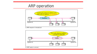
An ARP requestis broadcast;
an ARP reply is unicast.
Note
135.
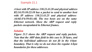
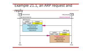
A host withIP address 130.23.43.20 and physical address
B2:34:55:10:22:10 has a packet to send to another host
with IP address 130.23.43.25 and physical address
A4:6E:F4:59:83:AB. The two hosts are on the same
Ethernet network. Show the ARP request and reply
packets encapsulated in Ethernet frames.
Solution
Figure 21.5 shows the ARP request and reply packets.
Note that the ARP data field in this case is 28 bytes, and
that the individual addresses do not fit in the 4-byte
boundary. That is why we do not show the regular 4-byte
boundaries for these addresses.
Example 21.1
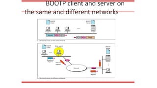
DHCP provides staticand dynamic
address allocation that can be
manual or automatic.
Note
140.
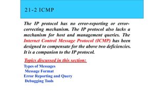
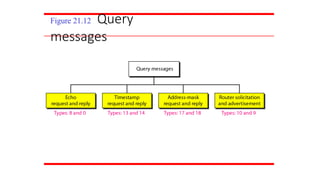
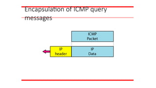
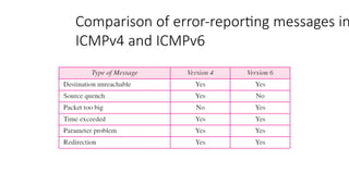
21-2 ICMP
The IPprotocol has no error-reporting or error-
correcting mechanism. The IP protocol also lacks a
mechanism for host and management queries. The
Internet Control Message Protocol (ICMP) has been
designed to compensate for the above two deficiencies.
It is a companion to the IP protocol.
Topics discussed in this section:
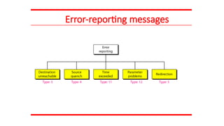
Types of Messages
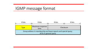
Message Format
Error Reporting and Query
Debugging Tools
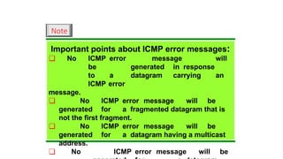
Important points aboutICMP error messages:
❏ No ICMP error message will
be generated in response
to a datagram carrying an
ICMP error
message.
❏ No ICMP error message will be
generated for a fragmented datagram that is
not the first fragment.
❏ No ICMP error message will be
generated for a datagram having a multicast
address.
❏ No ICMP error message will be
Note
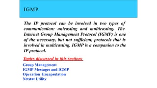
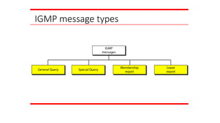
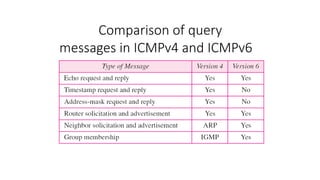
IGMP
The IP protocolcan be involved in two types of
communication: unicasting and multicasting. The
Internet Group Management Protocol (IGMP) is one
of the necessary, but not sufficient, protocols that is
involved in multicasting. IGMP is a companion to the
IP protocol.
Topics discussed in this section:
Group Management
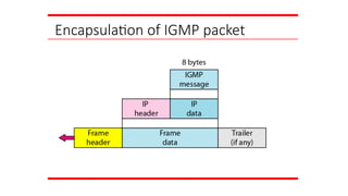
IGMP Messages and IGMP
Operation Encapsulation
Netstat Utility
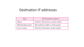
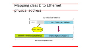
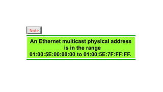
An Ethernet multicastphysical address
is in the range
01:00:5E:00:00:00 to 01:00:5E:7F:FF:FF.
Note
161.
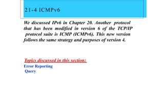
21-4 ICMPv6
We discussedIPv6 in Chapter 20. Another protocol
that has been modified in version 6 of the TCP/IP
protocol suite is ICMP (ICMPv6). This new version
follows the same strategy and purposes of version 4.
Topics discussed in this section:
Error Reporting
Query
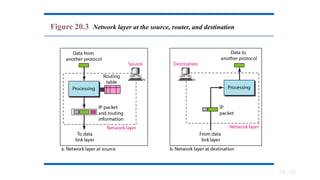
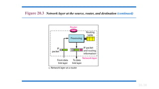
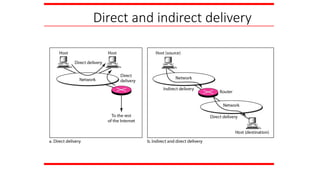
22-1 DELIVERY
The networklayer supervises the handling of the
packets by the underlying physical networks. We
define this handling as the delivery of a packet.
Topics discussed in this section:
Direct Versus Indirect Delivery
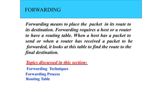
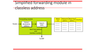
FORWARDING
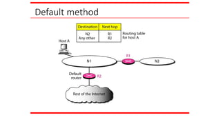
Forwarding means toplace the packet in its route to
its destination. Forwarding requires a host or a router
to have a routing table. When a host has a packet to
send or when a router has received a packet to be
forwarded, it looks at this table to find the route to the
final destination.
Topics discussed in this section:
Forwarding Techniques
Forwarding Process
Routing Table
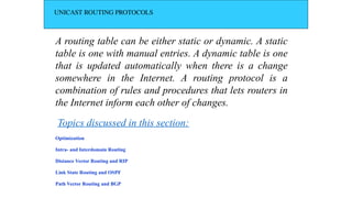
UNICAST ROUTING PROTOCOLS
Arouting table can be either static or dynamic. A static
table is one with manual entries. A dynamic table is one
that is updated automatically when there is a change
somewhere in the Internet. A routing protocol is a
combination of rules and procedures that lets routers in
the Internet inform each other of changes.
Optimization
Intra- and Interdomain Routing
Distance Vector Routing and RIP
Link State Routing and OSPF
Path Vector Routing and BGP
Topics discussed in this section:
173.
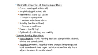
Desirable propertiesof Routing Algorithms:
Correctness (applicable to all)
Simplicity (applicable to all)
Robustness: able to cope up with
changes in topology, load.
hardware and software failures
Stability (hard to achieve)
Converge to equilibrium
Fairness (conflicting)
Optimality (conflicting) see next fig.
Types of Routing Algorithms:
Non-Adaptive: Static. Routing decisions computed in advance,
off-line and downloaded.
Adaptive: Dynamic. Adaptive to the changes in topology and
load. Issue here is how to get the information? Locally, From
adjacent routers, from all routers?
174.
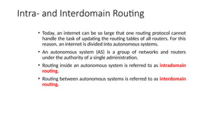
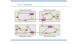
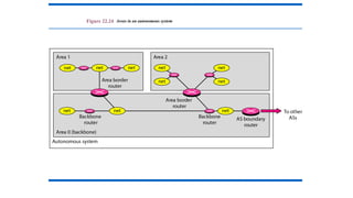
Intra- and InterdomainRouting
• Today, an internet can be so large that one routing protocol cannot
handle the task of updating the routing tables of all routers. For this
reason, an internet is divided into autonomous systems.
• An autonomous system (AS) is a group of networks and routers
under the authority of a single administration.
• Routing inside an autonomous system is referred to as intradomain
routing.
• Routing between autonomous systems is referred to as interdomain
routing.
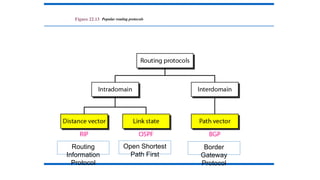
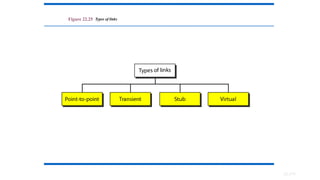
Figure 22.13 Popularrouting protocols
Routing
Information
Protocol
Open Shortest
Path First
Border
Gateway
Protocol
177.
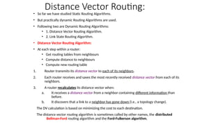
Distance Vector Routing:
•So far we have studied Static Routing Algorithms.
• But practically dynamic Routing Algorithms are used.
• Following two are Dynamic Routing Algorithms:
• 1. Distance Vector Routing Algorithm.
• 2. Link State Routing Algorithm.
• Distance Vector Routing Algorithm:
• At each step within a router:
• Get routing tables from neighbours
• Compute distance to neighbours
• Compute new routing table
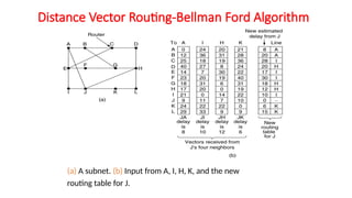
1. Router transmits its distance vector to each of its neighbors.
2. Each router receives and saves the most recently received distance vector from each of its
neighbors.
3. A router recalculates its distance vector when:
a. It receives a distance vector from a neighbor containing different information than
before.
b. It discovers that a link to a neighbor has gone down (i.e., a topology change).
The DV calculation is based on minimizing the cost to each destination.
The distance vector routing algorithm is sometimes called by other names, the distributed
Bellman-Ford routing algorithm and the Ford-Fulkerson algorithm.
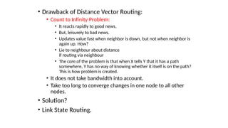
• Drawback ofDistance Vector Routing:
• Count to Infinity Problem:
• It reacts rapidly to good news,
• But, leisurely to bad news.
• Updates value fast when neighbor is down, but not when neighbor is
again up. How?
• Lie to neighbour about distance
if routing via neighbour
• The core of the problem is that when X tells Y that it has a path
somewhere, Y has no way of knowing whether it itself is on the path?
This is how problem is created.
• It does not take bandwidth into account.
• Take too long to converge changes in one node to all other
nodes.
• Solution?
• Link State Routing.
180.
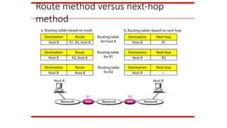
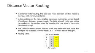
Distance Vector Routing
•In distance vector routing, the least-cost route between any two nodes is
the route with minimum distance.
• In this protocol, as the name implies, each node maintains a vector (table)
of minimum distances to every node. The table at each node also guides
the packets to the desired node by showing the next stop in the route
(next-hop routing).
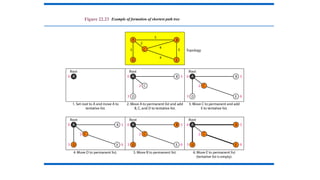
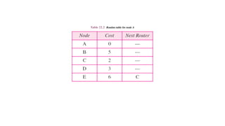
• The table for node A shows how to reach any node from this node. For
example, our least cost to reach node E is 6. The route passes through C.
• Routing Table:
22.180
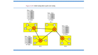
22.182
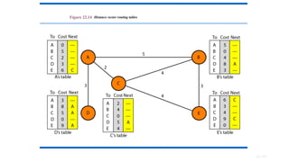
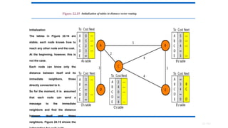
Figure 22.15 Initializationof tables in distance vector routing
Initialization
The tables in Figure 22.14 are
stable; each node knows how to
reach any other node and the cost.
At the beginning, however, this is
not the case.
Each node can know only the
distance between itself and its
immediate neighbors, those
directly connected to it.
So for the moment, it is assumed
that each node can send a
message to the immediate
neighbors and find the distance
between itself and these
neighbors. Figure 22.15 shows the
183.
In distance vectorrouting, each node shares its routing table with its
immediate neighbors periodically and when there is a change.
Note
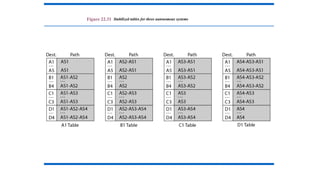
184.
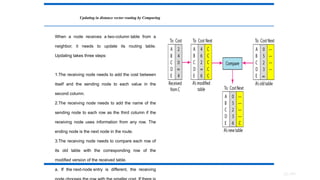
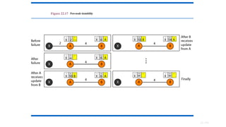
22.184
Updating in distancevector routing by Comparing
When a node receives a two-column table from a
neighbor, it needs to update its routing table.
Updating takes three steps:
1.The receiving node needs to add the cost between
itself and the sending node to each value in the
second column.
2.The receiving node needs to add the name of the
sending node to each row as the third column if the
receiving node uses information from any row. The
ending node is the next node in the route.
3.The receiving node needs to compare each row of
its old table with the corresponding row of the
modified version of the received table.
a. If the next-node entry is different, the receiving
185.
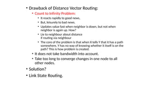
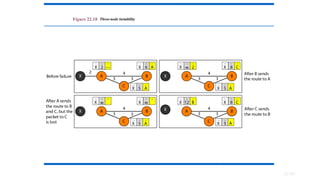
• Drawback ofDistance Vector Routing:
• Count to Infinity Problem:
• It reacts rapidly to good news,
• But, leisurely to bad news.
• Updates value fast when neighbor is down, but not when
neighbor is again up. How?
• Lie to neighbour about distance
if routing via neighbour
• The core of the problem is that when X tells Y that it has a path
somewhere, Y has no way of knowing whether it itself is on the
path? This is how problem is created.
• It does not take bandwidth into account.
• Take too long to converge changes in one node to all
other nodes.
• Solution?
• Link State Routing.
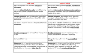
Link State DistanceVector
link states algorithm is an algorithm using global
information
the distance vector algorithm is iterative, asynchronous,
and distributed
each node talks with all other nodes, but tell them only
the cost of it's directly comparison of some of their
attribute
each node talks to only its directly connected neighbors,
but provides its neighbor with least cost estimates from
itself to all the nodes.
Message complexity: With link state, every node has to
keep the information about the cost of each link within
the network.
Message complexity: with distance vector algorithm,
message is exchanged between two hosts which are
directly connected to each other.
very times, if any of the link cost is changed, all the nodes
are updated.
change of cost in the link which is belong to the least cost
path for one of the nodes, the DV algorithm will update
the new value. But if the change doesn't belong to the
least cost part between 2 hosts, there will no updating.
Speed of convergence: can converge faster in comparison
of later.
Speed of convergence: can converge slowly and have
routing loops while the algorithm is converging.
Such probability is less. DV algorithm also suffers from the count to infinity
problem.
Robustness: For LS, when a router is down, it can
broadcast a wrong cost for the closest one. LS node is
computing for its own forwarding table and other node do
the calculation for themselves. Better than DV.
Robustness: DV, the wrong least cost path can be passed
to more than one or all of the node so the wrong
calculation will be process in the entire net work. This
problem of DV is much worse than LS algorithm.
189.
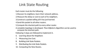
Link State Routing
Eachrouter must do the following:
1.Discover its neighbors, learn their network address.
2.Measure the delay or cost to each of its neighbors.
3.Construct a packet telling all it has just learned.
4.Send this packet to all other routers.
5.Compute the shortest path to every other router.
A complete topology is developed. Then Dijkstra’s Algorithm can be used to
compute the shortest path.
Following 5 steps are followed to implement it.
6. Learning about the Neighbors
7. Measuring Line Cost.
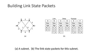
8. Building Link State Packets.
9. Distributing the Link State Packets.
10. Computing the New Routes.
190.
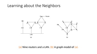
Learning about theNeighbors
(a) Nine routers and a LAN. (b) A graph model of (a).
191.
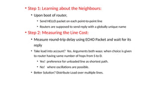
• Step 1:Learning about the Neighbours:
• Upon boot of router,
• Send HELLO packet on each point-to-point line
• Routers are supposed to send reply with a globally unique name
• Step 2: Measuring the Line Cost:
• Measure round-trip delay using ECHO Packet and wait for its
reply
• Take load into account? Yes. Arguments both ways: when choice is given
to router having same number of hops from S to D.
• Yes! preference for unloaded line as shortest path.
• No! where oscillations are possible.
• Better Solution? Distribute Load over multiple lines.
192.
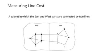
Measuring Line Cost
Asubnet in which the East and West parts are connected by two lines.
193.
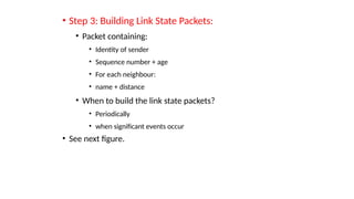
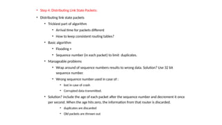
• Step 3:Building Link State Packets:
• Packet containing:
• Identity of sender
• Sequence number + age
• For each neighbour:
• name + distance
• When to build the link state packets?
• Periodically
• when significant events occur
• See next figure.
194.
Building Link StatePackets
(a) A subnet. (b) The link state packets for this subnet.
195.
• Step 4:Distributing Link State Packets:
• Distributing link state packets
• Trickiest part of algorithm
• Arrival time for packets different
• How to keep consistent routing tables?
• Basic algorithm
• Flooding +
• Sequence number (in each packet) to limit duplicates.
• Manageable problems
• Wrap around of sequence numbers results to wrong data. Solution? Use 32 bit
sequence number.
• Wrong sequence number used in case of :
• lost in case of crash
• Corrupted data transmitted.
• Solution? include the age of each packet after the sequence number and decrement it once
per second. When the age hits zero, the information from that router is discarded.
• duplicates are discarded
• Old packets are thrown out
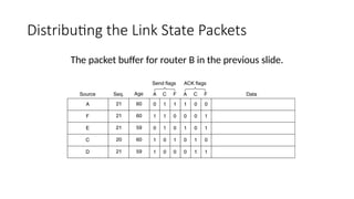
196.
Distributing the LinkState Packets
The packet buffer for router B in the previous slide.
197.
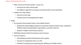
Step 5: Computingnew routes:
• With a full set of link state packets, a router can:
• Construct the entire subnet graph
• Run Dijkstra’s algorithm to compute the shortest path to each destination
• Problems for large subnets
• Memory to store data
• Compute time for developing these tables.
• Usage:
• IS-IS protocol (Intermediate System, Intermediate System)
• Designed for DECnet(digital equipment corporation network protocol suite), adopted by
ISO(international standardization organization), used still in internet.
• Supports multiple network layer protocols
• OSPF(Open Shortest Path First) protocol used in Internet
• Common features:
• Self-stabilizing method of flooding link state updates
• Concept of a designated router on a LAN
• Method of computing and supporting path splitting and multiple metrics.
198.
Link State Routing
•Previous Distance vector routers use a distributed algorithm to compute
their routing tables, link-state routing uses link-state routers to exchange
messages that allow each router to learn the entire network topology.
Based on this each router is then able to compute its routing table by using
a shortest path computation.
• Features of link state routing protocols –
• Link state packet – A small packet that contains routing information.
• Link state database – A collection information gathered from link state
packet.
• Shortest path first algorithm (Dijkstra algorithm) – A calculation
performed on the database results into shortest path
• Routing table – A list of known paths and interfaces.
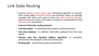
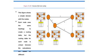
199.
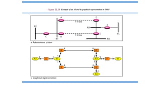
Figure 22.20 Conceptof link state routing
• This figure shows
a simple domain
with five nodes.
• Each node uses
the same
topology to
create a routing
table, but the
routing table for
each node is
unique because
the calculations
are based on
different
200.
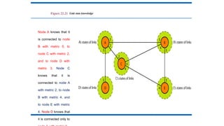
Figure 22.21 Linkstate knowledge
Node A knows that it
is connected to node
B with metric 5, to
node C with metric 2,
and to node D with
metric 3. Node C
knows that it is
connected to node A
with metric 2, to node
B with metric 4, and
to node E with metric
4. Node D knows that
it is connected only to
201.
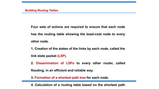
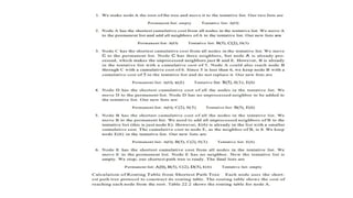
Building Routing Tables
Foursets of actions are required to ensure that each node
has the routing table showing the least-cost node to every
other node.
1. Creation of the states of the links by each node, called the
link state packet (LSP).
2. Dissemination of LSPs to every other router, called
flooding, in an efficient and reliable way.
3. Formation of a shortest path tree for each node.
4. Calculation of a routing table based on the shortest path
202.
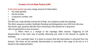
Creation of LinkState Packet (LSP)
A link state packet can carry a large amount of information
• the node identity,
• the list of links,
• a sequence number, and
• age.
The first two, node identity and the list of links, are needed to make the topology.
The third, sequence number, facilitates flooding and distinguishes new LSPs from old ones.
The fourth, age, prevents old LSPs from remaining in the domain for a long time.
LSPs are generated on two occasions:
1. When there is a change in the topology ofthe domain. Triggering of LSP
dissemination is the main way of quickly informing any node in the domain to update its
topology.
2. On a periodic basis. It is done to ensure that old information is removed from the
domain. The timer set for periodic dissemination is normally in the range of 60 min or 2 h
based on the implementation.
203.
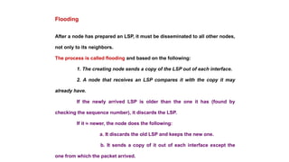
After a nodehas prepared an LSP, it must be disseminated to all other nodes,
not only to its neighbors.
The process is called flooding and based on the following:
1. The creating node sends a copy of the LSP out of each interface.
2. A node that receives an LSP compares it with the copy it may
already have.
If the newly arrived LSP is older than the one it has (found by
checking the sequence number), it discards the LSP.
If it is newer, the node does the following:
a. It discards the old LSP and keeps the new one.
b. It sends a copy of it out of each interface except the
one from which the packet arrived.
Flooding
204.
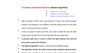
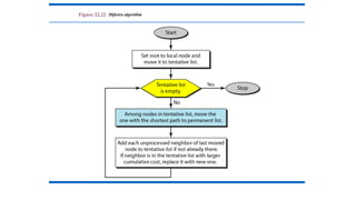
Formation of ShortestPath Tree (Dijkstra Algorithm):
• After receiving all LSPs, each node will have a copy of the whole topology.
However, the topology is not sufficient to find the shortest path to every other
node; a shortest path tree is needed.
• A tree is a graph of nodes and links; one node is called the root. All other
nodes can be reached from the root through only one single route.
• A shortest path tree is a tree in which the path between the root and
every other node is the shortest.
• The Dijkstra algorithm creates a shortest path tree from a graph.
• The algorithm divides the nodes into two sets: tentative and permanent.
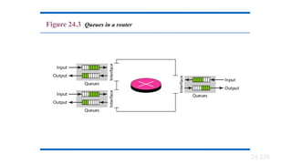
a. Minimize mean packet delay
b. Maximize the network throughput
c. Minimize the number of hops along the path
DATA TRAFFIC
The mainfocus of congestion control and quality of
service is data traffic. In congestion control we try to
avoid traffic congestion. In quality of service, we try to
create an appropriate environment for the traffic. So,
before talking about congestion control and quality of
service, we discuss the data traffic itself.
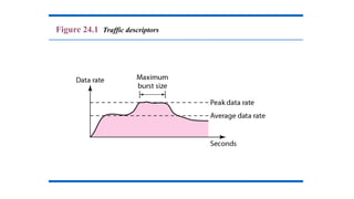
Traffic Descriptor
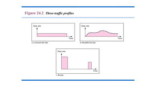
Traffic Profiles
Topics discussed in this section:
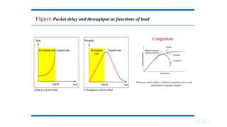
CONGESTION
Congestion in anetwork may occur if the load on the
network—the number of packets sent to the network—is
greater than the capacity of the network—the number of
packets a network can handle. Congestion control refers
to the mechanisms and techniques to control the
congestion and keep the load below the capacity.
Network Performance
Topics discussed in this section:
223.
Congestion Control Introduction:
•When too many packets are present in (a part of) the subnet, performance
degrades. This situation is called congestion.
• As traffic increases too far, the routers are no longer able to cope and they
begin losing packets.
• At very high traffic, performance collapses completely and almost no
packets are delivered.
• Reasons of Congestion:
• Slow Processors.
• High stream of packets sent from one of the sender.
• Insufficient memory.
• High memory of Routers also add to congestion as becomes un manageable and
un accessible. (Nagle, 1987).
• Low bandwidth lines.
• Then what is congestion control? Congestion control has to do with
making sure the subnet is able to carry the offered traffic.
• Congestion control and flow control are often confused but both helps
reduce congestion.
224.
General Principles ofCongestion Control
• Three Step approach to apply congestion control:
1.Monitor the system .
• detect when and where congestion occurs.
2.Pass information to where action can be taken.
3.Adjust system operation to correct the problem.
• How to monitor the subnet for congestion.
1) percentage of all packets discarded for lack of buffer space,
2) average queue lengths,
3) number of packets that time out and are retransmitted,
4) average packet delay
5) standard deviation of packet delay (jitter Control).
225.
• Knowledge ofcongestion will cause the hosts to take appropriate action to reduce the congestion.
• For a scheme to work correctly, the time scale must be adjusted carefully.
• If every time two packets arrive in a row, a router yells STOP and every time a router is idle for 20
µsec, it yells GO, the system will oscillate wildly and never converge.
• Dividing all algorithms into
• open loop or
• closed loop
• They further divide the open loop algorithms into ones that act at the source versus ones that act
at the destination.
• The closed loop algorithms are also divided into two subcategories:
• explicit feedback implicit feedback.
• In explicit feedback algorithms, packets are sent back from the point of congestion to warn
the source.
• In implicit algorithms, the source deduces the existence of congestion by making local
observations, such as the time needed for acknowledgements to come back.
• The presence of congestion means that the load is (temporarily) greater than the resources can
handle.
• Solution?
• increase the resources or
• decrease the load.
• That is not always possible. So we have to apply some congestion prevention policy.
24.228
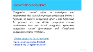
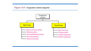
CONGESTION CONTROL
Congestion controlrefers to techniques and
mechanisms that can either prevent congestion, before it
happens, or remove congestion, after it has happened.
In general, we can divide congestion control
mechanisms into two broad categories: open-loop
congestion control (prevention) and closed-loop
congestion control (removal).
Open-Loop Congestion Control
Closed-Loop Congestion Control
Topics discussed in this section:
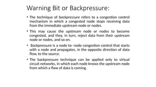
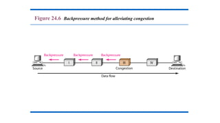
Warning Bit orBackpressure:
• The technique of backpressure refers to a congestion control
mechanism in which a congested node stops receiving data
from the immediate upstream node or nodes.
• This may cause the upstream node or nodes to become
congested, and they, in turn, reject data from their upstream
node or nodes, and so on.
• Backpressure is a node to- node congestion control that starts
with a node and propagates, in the opposite direction of data
flow, to the source.
• The backpressure technique can be applied only to virtual
circuit networks, in which each node knows the upstream node
from which a flow of data is coming.
231.
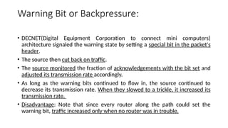
Warning Bit orBackpressure:
• DECNET(Digital Equipment Corporation to connect mini computers)
architecture signaled the warning state by setting a special bit in the packet's
header.
• The source then cut back on traffic.
• The source monitored the fraction of acknowledgements with the bit set and
adjusted its transmission rate accordingly.
• As long as the warning bits continued to flow in, the source continued to
decrease its transmission rate. When they slowed to a trickle, it increased its
transmission rate.
• Disadvantage: Note that since every router along the path could set the
warning bit, traffic increased only when no router was in trouble.
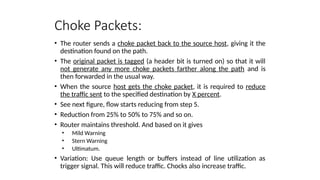
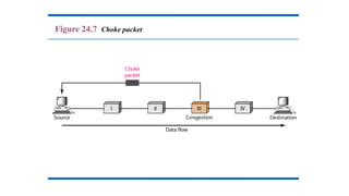
Choke Packets:
• Therouter sends a choke packet back to the source host, giving it the
destination found on the path.
• The original packet is tagged (a header bit is turned on) so that it will
not generate any more choke packets farther along the path and is
then forwarded in the usual way.
• When the source host gets the choke packet, it is required to reduce
the traffic sent to the specified destination by X percent.
• See next figure, flow starts reducing from step 5.
• Reduction from 25% to 50% to 75% and so on.
• Router maintains threshold. And based on it gives
• Mild Warning
• Stern Warning
• Ultimatum.
• Variation: Use queue length or buffers instead of line utilization as
trigger signal. This will reduce traffic. Chocks also increase traffic.
Implicit Signalling Inimplicit signalling, there is no
communication between the congested node or nodes and the
source. The source guesses that there is congestion somewhere
in the network from other symptoms. For example, when a
source sends several packets and there is no acknowledgment
for a while, one assumption is that the network is congested.
The delay in receiving an acknowledgment is interpreted as
congestion in the network; the source should slow down.
Explicit Signalling The node that experiences congestion can
explicitly send a signal to the source or destination. The
explicit-signalling method, however, is different from the
choke-packet method. In the choke-packet method, a separate
packet is used for this purpose; in the explicit-signalling
method, the signal is included in the packets that carry data.
Explicit signalling can occur in either the forward or the
backward direction. This type of congestion control can be seen
236.
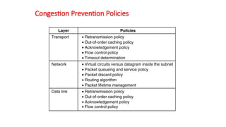
1. Retransmission Policy:It is the policy in which retransmission of
the packets are taken care. If the sender feels that a sent packet is lost or
corrupted, the packet needs to be retransmitted. This transmission may
increase the congestion in the network. To prevent congestion,
retransmission timers must be designed to prevent congestion and also
able to optimize efficiency.
2. Window Policy: The type of window at the sender side may also
affect the congestion. Several packets in the Go-back-n window are
resent, although some packets may be received successfully at the
receiver side. This duplication may increase the congestion in the
network and making it worse. Therefore, Selective repeat window
should be adopted as it sends the specific packet that may have been
lost.
Open Loop Congestion Control
237.
3. Discarding Policy:A good discarding policy adopted by the routers is
that the routers may prevent congestion and at the same time partially
discards the corrupted or less sensitive package and also able to maintain
the quality of a message. In case of audio file transmission, routers can
discard less sensitive packets to prevent congestion and also maintain the
quality of the audio file.
4. Acknowledgment Policy: Since acknowledgement are also the part of
the load in network, the acknowledgment policy imposed by the receiver
may also affect congestion. Several approaches can be used to prevent
congestion related to acknowledgment. The receiver should send
acknowledgement for N packets rather than sending acknowledgement for
a single packet. The receiver should send a acknowledgment only if it has
to send a packet or a timer expires.
5. Admission Policy: In admission policy a mechanism should be used to
prevent congestion. Switches in a flow should first check the resource
requirement of a network flow before transmitting it further. If there is a
chance of a congestion or there is a congestion in the network, router
should deny establishing a virtual network connection to prevent further
congestion.
Open Loop Congestion Control