This document presents a study on improving clock synchronization in clustered wireless sensor networks using a combination of truncated mean and whale optimization techniques. The proposed approach aims to enhance synchronization accuracy by grouping sensor nodes into non-overlapping clusters and employing multi-hop message exchange for synchronization. Simulation results indicate that the new method outperforms existing protocols by achieving lower synchronization errors and reduced communication overhead.
![International Journal of Computer Networks & Communications (IJCNC) Vol.13, No.3, May 2021
DOI: 10.5121/ijcnc.2021.13304 57
CLOCK SYNCHRONIZATION USING TRUNCATED
MEAN AND WHALE OPTIMIZATION FOR
CLUSTERED SENSOR NETWORKS
Karthik Soundarapandian1
and Ashok Kumar Ambrose2
1
Research Scholar, Research and Development Centre,
Bharathiar University, Coimbatore, Tamilnadu, India
2
Assistant Professor, Department of Computer Science,
Alagappa Govt. Arts College, Karaikudi, Tamilnadu, India
ABSTRACT
Clock synchronization is an important component in many distributed applications of wireless sensor
networks (WSNs). The deprived method of clock offset and skew estimation causes inaccuracy,
synchronization delay, and communication overhead in the protocols. Hence, this paper exploits two
techniques of variation truncated mean (VTM) and whale optimization (WO) to enhance the
synchronization metrics. Sensor nodes are grouped into several non-overlapped clusters. The cluster head
collects the member nodes’ local time and computes the synchronization time 𝑆𝑍𝑡 using the truncated
mean method. Nodes with a high variation in the timings compared to a preset value are truncated. The
head node broadcasts the 𝑆𝑍𝑡 in which the whale optimization is aiming at each node to reduce the
synchronization error. The intra and inter-cluster synchronizations are accomplished through the multi-
hop message exchange approach. The theoretical analysis is validated, and the simulation outcomes show
that the performance metrics in the proposed work are better than the conventional methods by achieving
minimum error value.
KEYWORDS
Clustering, Clock Synchronization, Truncated Mean, Whale Optimization, Clock Time Duration.
1. INTRODUCTION
The research focus on the sensor network domain has extensively increased for the use of
prospective applications such as target tracking, industrial automation, area monitoring, military,
and landslide detection. In these applications, nodes are necessitated to maintain a standard time
to specify the timing of events [1]. Therefore, the clocks of the sensor nodes (SNs) are vital to
synchronize which allows the entire network to collaborate and imparts reliable seamless
communication between the nodes without delay. Time synchronization (TS) is a critical
middleware package that requires consistent distribution sensing and control over large-scale
sensor networks. TS may not be required in the centralized networks as there is no uncertainty.
Over the past few years, several protocols have been proposed to address the synchronization
problem like precision, computational complexity, node failure, and energy consumption [2].
The sensors’ hardware clocks are imperfect and functioning at particular frequencies. Since nodes
are deployed randomly at different positions, the temperature fluctuations may cause the clock to
slow down or speed up. The frequency is the speed of clock ticks, and its alteration in the logical
clocks minimizes the error [3]. Sensors maintain their clocks and sometimes obtain disparate](https://image.slidesharecdn.com/13321cnc04-210630084404/85/Clock-Synchronization-using-Truncated-Mean-and-Whale-Optimization-for-Clustered-Sensor-Networks-1-320.jpg)
![International Journal of Computer Networks & Communications (IJCNC) Vol.13, No.3, May 2021
58
timings due to: (i) clocks if started at different times (ii) quartz crystals in nodes might have been
acted on different frequencies causing the clock values to diverge from each other, and (iii) the
frequency of the clocks change over the time due to aging or ambient conditions. The nodes
initiate the synchronization process periodically based on the clock readings, and the
communication delay between two linked nodes is excluded in the delay-free case model [4,5].
The lifetime of synchronization is the amount of time that nodes maintain the clock readings
consistently. Synchronization can be either global, where the timings are equalized in all the
nodes, or local, that is equalization barely in a set of nodes. Though the clocks are synchronized
by the message exchange method, packets are also to be synchronized before the transmission
because sensed data often loses valuable context without accurate time information [6]. The
synchronization shall be based on either a sender-receiver or receiver-receiver approach and
accomplished via one-way message passing, multi-way broadcasting, and pair-wise
synchronization. It is also possible with a timestamp technique that most of the TS protocols
required [7-9].
Cluster-based sensor networks can perform accurate synchronization efficiently. The clustering
technique has been extensively used to solve most of the synchronization issues. The clusters
consist of cluster heads (CHs) and member nodes (MNs). The head nodes are initially
synchronized to the base station (BS), and children nodes synchronize with their heads [10,11].
Such a method of synchronization eradicates message replication that enhances the convergence
rate compared to the traditional topology. The synchronization protocols are categorized into
reference and distributed-based models. The reference node comprises a pre-defined structure to
attain network-wide synchronization whereas, nodes are distributed to scale and robust the entire
network topology. In [12-14], reference nodes are acting as superior nodes that broadcast the
synchronization message with timing information over the neighbours to cover the environment.
A network that has minimal reference nodes reduces the energy dissipation drastically because it
acquires a lesser number of communications. TS protocols have also been developed using
consensus-based technique [15,16]. The concept of consensus is achieving trustworthiness by
involving multiple distributed nodes containing the same time information. The determination of
drift and skew errors, message delay, and oscillation of clock speed are neither designed nor
discussed in the consensus-based synchronization. The robust TS [17] is developed based on
maximum consensus considering the estimation and compensation of errors. As much as the
offset and skew errors are minimized, the synchronization accuracy is increased.
The synchronization delay occurs by the accounting of transmission and propagation times and
reduced at the sender and receiver nodes using the timestamp method that is efficiently devised
based upon a linear clock model [18]. The synchronization process is incomplete if a parent node
or reference node fails. Therefore, the dynamic method of selection may be an optimal solution to
avoid failure. The recovery of data packets from the failure nodes is a challenging task in the
synchronization phase. A protocol called self-recoverable TS [19] adopts a candidate node as a
timer to check whether the synchronization is over. It selects a new root node by considering the
energy level. The single-hop neighbouring pair-wise average transmission gives a quite
difference in timings for the large-sized network. Due to this reason, multi-hop pair-wise
synchronization with a short route is considered to transmit the sync messages. Also, the on-
demand method [20] is adopted for a mutual coordination (a reactive mechanism) in a multi-hop
communication. The propagation of a sync message may increase the message complexity either
if the sensing area is enlarged or network size is increased [21].
In this paper, we develop a cluster-based VTM-WO protocol to solve the addressed problems of
synchronization. The clock time is not modified, and there is no virtual clock in the proposed
work. The sync packets are recorded by the clock time duration (CTD) model. The major
contributions of our proposed work are the followings:](https://image.slidesharecdn.com/13321cnc04-210630084404/85/Clock-Synchronization-using-Truncated-Mean-and-Whale-Optimization-for-Clustered-Sensor-Networks-2-320.jpg)
![International Journal of Computer Networks & Communications (IJCNC) Vol.13, No.3, May 2021
59
A standard procedure of the clustering process for energy-efficient transmission.
Truncated mean method for clock parameters (offset and skew) estimation.
Multi-hop based synchronization with fewer messages overhead.
Whale optimization technique to reduce the synchronization error in both intra and
inter-cluster communications.
Evaluation of synchronization metrics to show the performance of the proposed work
with conventional algorithms.
The rest of the paper is organized as follows: Section 2 presents the existing protocols for time
synchronization and the problem statement. In section 3, the network and clock models are
discussed under system setup. The proposed VTM-WO protocol for intra and inter-cluster
synchronizations is described in section 4. Section 5 illustrates the simulation results of the
performance parameters. At last, the conclusion is given in section 6.
2. RELATED WORK AND PROBLEM STATEMENT
Time is an imperative factor in network operations. The sensor’s clock is defined as a time
calculator and a layer of the network architecture. Nodes’ looping a time division multiple access
(TDMA) protocol must agree for the time slots to avoid collision and overlapping hence,
synchronization becomes essential for any successful event. This section discusses the recent
works and problems related to synchronization in the distributed environment.
J. Wang, et al., [22] proposed the two-hop time synchronization (TTS) protocol for sensory
networks where synchronization overhead is highly reduced. In TTS, the reference node records
the timestamp, and the parent node synchronizes with the children nodes through two-way timing
messages. The synchronization error is reduced by involving the minimum relay nodes. The
problem with the protocol is much sensitive while changing the network size that led to more
delays in the synchronization process. The clustering technique has been integrated into
consensus-based time synchronization (CCTS) algorithm [23] to eradicate the message
replications. The algorithm consists of two phases: (i) intra-cluster synchronization where the
skew and offset parameters are updated by the average value of the virtual clocks (ii) inter-cluster
synchronization in which head nodes' are assigned with weights based on the cluster sizes. The
algorithm achieves faster convergence and better energy consumption. In CCTS, the
synchronization error is not addressed due to the deprived method of clock estimation delay.
Clock skew is one of the important attributes for better accurate synchronization. F. Shi, et al.,
[24] presented maximum likelihood estimation (MLE) algorithm to reduce the skew convergence
error based on the Gaussian distribution delay and multiple one-way broadcast models. The MLE
performs accurate estimation of skew, quick convergence speed, and energy-efficient. Results for
other synchronization parameters are not carried to analyze the overall performance of the
algorithm. In [25], a field-programmable gate array (FPGA) method is introduced for
timestamping pertained to reference broadcast synchronization (RBS). The authors also proposed
a dynamic adjusting time synchronization (DATS) protocol for compensating the node clocks
continuously through dynamic adjustments (coarse and fine). It does not work well for a large-
scale network during the synchronization phase. The prediction scheme over the skew or offset
error in time synchronization does not modify or readjust in any of the parameters. H. Wang, et
al., [26] employed a linear Gaussian delay model to estimate the skew convergence and aimed to
adjust the clock immediately using a multi-hop approach. At every round of synchronization, a
one-way timing message is distributed, and skew is estimated without considering the delay
element. The message overhead and energy consumption are raised due to multiple intermediate
nodes. The use of pulse-coupled synchronization to an acoustic event detection system for a](https://image.slidesharecdn.com/13321cnc04-210630084404/85/Clock-Synchronization-using-Truncated-Mean-and-Whale-Optimization-for-Clustered-Sensor-Networks-3-320.jpg)
![International Journal of Computer Networks & Communications (IJCNC) Vol.13, No.3, May 2021
60
wireless sensor network is presented by Nunez, F et al [27]. It aims at finding the source of
acoustic events using the arrival time and also facilitates the accurate distributed localization even
if there is a clock drift between the nodes. Each sensor creates a variable that increases at a
specified rate by the frequency. The variable is initialized with the incoming pulses and
broadcasts them to the neighbours. The authors use the consensus synchronization technique to
attain both localization and synchronization through simple communication. In this algorithm, the
mean absolute error (MAE) is not minimized in all the cases, and also the accurate localization is
not compensated.
A single-hop communication in consensus-based algorithms performs defective results for both
accuracy and convergence speed. N. Panigrahi and P.M. Khilar, [28] have proposed a consensus-
based selective average time synchronization (SATS) algorithm for multi-hop networks. The
algorithm effectively enhances the topological connectivity and restricts the end-to-end delay
through a constraint-based dynamic programming approach. The multi-hop SATS is equipped
with a rapid convergence however, message complexity is high. In [29], cluster-based
synchronization is addressed called energy-based proportional integral and least common
multiple (EPILCM) protocol. It compares the node’s time with the reference clock and if there is
any difference then, computes the propagation delay. The clock parameters are compensated
using a proportional-integral controller, and the consensus-based synchronization is performed by
the LCM method. The processing time of synchronization is relatively high in EPILCM.
G.S.S. Chalapathi, et al., [30] proposed an efficient and simple algorithm for time
synchronization (E-SATS) to minimize the synchronization error and energy consumption in two
different environments. In E-SATS, clusters are formulated by the head nodes, and the joining
packets are broadcasted. If a node collects more than one acknowledgment from the heads such
node becomes a gateway node. After the clustering process, the head node transmits a
synchronization packet to its members containing a timestamp. All member nodes record the
reception time and sending the acknowledgment packets after a pre-determined time. The clock
skew and offset error rate are not methodologically computed thus, increase the synchronization
complexity, and also precision is defected by the delay. In [31], rapid-flooding multi-broadcast
time synchronization with real-time delay compensation is presented to reduce the packet delay
in a high-density network. The protocol broadcast the redundant packets and estimate the
accurate offset-skew using MLE. Also, a two-way exchange model is used to guarantee the delay
estimate and the precision. The energy wastage is more due to message overhead.
We have addressed the problems of all the above existing synchronization protocols in this
section. The lack of a solution to these problems and limitations motivated us to propose a
proficient protocol for the clock synchronization component.
3. SYSTEM SETUP
The network is designed with the homogeneity of nodes where the base station is situated within
the sensing environment. The clusters are non-overlapped by considering the overall energy
consumption of the network. Both intra and inter-cluster synchronizations are executed based on
the sender-receiver approach. The TDMA protocol is invoked to avoid the same time event
occurrence in the multi-hop messages transmission. The section discusses the network depiction
in a matrix structure, the method of clustering, and the CTD timestamp model for the cluster
synchronization.](https://image.slidesharecdn.com/13321cnc04-210630084404/85/Clock-Synchronization-using-Truncated-Mean-and-Whale-Optimization-for-Clustered-Sensor-Networks-4-320.jpg)
![International Journal of Computer Networks & Communications (IJCNC) Vol.13, No.3, May 2021
61
3.1. Network Model
The sensing field is assumed as a random graph 𝐺 = (𝑉, 𝐸), where 𝑉 symbolizes the group of
nodes and 𝐸 represents the link matrix between the neighbouring nodes. The node is indexed by
𝑛 and it ranges from 𝑣1 to 𝑣𝑛 that is expressed by 𝑣𝑛 ∈ 𝑉. When a node 𝑣𝑚 is in transmission
range with another node 𝑣𝑛 then, the link is created as 𝑙𝑚𝑛 = 1 otherwise, 𝑙𝑚𝑛 = 0, no
connection exists. Each node is uniquely identified in the network. The communication between
the linked nodes is symmetric, undirected, and static. The link 𝑙𝑚𝑛 between nodes is represented
in the 𝑉 × 𝑉 sparse matrix as:
𝐸 = [
𝑙11 ⋯ 𝑙1𝑛
⋮ ⋱ ⋮
𝑙𝑚1 ⋯ 𝑙𝑚𝑛
]
3.2. Clustering Phase
The clustering technique provides optimal energy utilization, lesser communication overhead,
and reduced crashing transmission. In this paper, non-overlapping clusters are formulated by
following our previously proposed REEC non-overlap protocol [10]. The steps for clustering are:
Step 1 : Initially, BS identifies the centroid of a square sensing environment.
Step 2 : BS calculates the average distance between the centroid and the nodes using the
euclidean metric.
Step 3 : 𝑘 number of clusters are determined using the energy communication model [32].
Step 4 : Mean points 𝑀 are initially selected for 𝑘 clusters.
Step 5 : Nodes are assigned to the closest 𝑀. This step is repeated until the static mean points
are met.
Step 6 : After the cluster construction, BS determines the cluster heads (CHs) for 𝑘 clusters
considering the rating value 𝑅𝑣 of sensor nodes. The 𝑅𝑣 is computed based upon the
three parameters such as available energy (AE), node’s degree (ND), and node’s
distance to BS (d_BS).
Step 7 : A node that has higher 𝑅𝑣 would be elected as a CH in the respective cluster. The CHs
are rotated to balance the energy and enhance the lifetime.
Such a method of clustering has proved as a better energy-efficient protocol in [10], and also
enhances the network lifetime, minimized delay, and maximized delivery ratio. Figure 1 shows
the clusters where the sensing area is 250 x 250 in meters, 𝑘 = 7 and BS (Sink node) is
positioned at 240 x 240 (m).](https://image.slidesharecdn.com/13321cnc04-210630084404/85/Clock-Synchronization-using-Truncated-Mean-and-Whale-Optimization-for-Clustered-Sensor-Networks-5-320.jpg)
![International Journal of Computer Networks & Communications (IJCNC) Vol.13, No.3, May 2021
62
Figure 1. Clusters with cluster heads
3.3. Clock Model
Typically, a node’s time 𝐶(𝑡) is composed of a local hardware-based crystal oscillator and a
counter [1]. Such a physical clock is used for tracking the current time of nodes in the sensor
network. At the initial stage, the time is set uniformly in all the nodes 𝑉 however; there will be a
drift in the clocks after a certain time due to signal variations. The local clock of actual initial
time 𝑡 in each sensor is mathematically given as:
𝐶(𝑡) = ∝ ∫ 𝜔(𝑡)
𝑡
0
𝑑𝑡 + 𝐶(𝑡0) (1)
where ∝ is a coefficient of proportionality, 𝜔(𝑡) denotes the oscillator’s angular frequency and
𝐶(𝑡0) represents the initial time of a sensor’s clock. In this paper, the communication is recorded
by a clock time duration (CTD) model as a timestamp shown in figure 2. The timestamp is an
important element to achieve synchronization, and to maintain the clocks. The CTD of a member
node 𝑛 and a head node ℎ is formulated by compiling both clocks offset and skew as:
𝐶𝑛(𝑡) = 𝐶ℎ(𝑡) = 𝜆𝑛 + 𝛾𝑛𝑡 (2)
where 𝜆𝑛 represents the clock offset that is a variation from the real time, and 𝛾𝑛 is the clock
skew that defines the clock frequency signal arrives at different components. Assume that there
are two nodes namely 𝑉1, and 𝑉2 with CTDs represented by 𝐶1(𝑡) and 𝐶2(𝑡)comprising
equivalent signal frequencies that is, expressed as:
𝛾1𝐶1(0) = 𝛾2𝐶2(0) (3)
The clocks offset and skew between two nodes 𝑉1 and 𝑉2 are computed using the following Eq.
(4) and Eq. (5):
𝜆𝑛 = |𝐶1(𝑡) − 𝐶2(𝑡)| = |𝜆1 − 𝜆2| (4)
𝛾𝑛 = |𝛾1𝐶1(𝑡) − 𝛾2𝐶2(𝑡)| (5)](https://image.slidesharecdn.com/13321cnc04-210630084404/85/Clock-Synchronization-using-Truncated-Mean-and-Whale-Optimization-for-Clustered-Sensor-Networks-6-320.jpg)
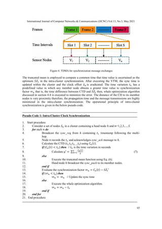
![International Journal of Computer Networks & Communications (IJCNC) Vol.13, No.3, May 2021
66
4.3. Multi-hop Inter-Cluster Synchronization Phase
The cluster heads that are closer to the base station can transmit the synchronization messages in
a single-hop however the distant nodes follow the multi-hop approach. All head nodes in the
inter-cluster do not receive the sync_message concurrently rather receive at different times and
records the timestamp. In intra-cluster, member nodes are synchronized in disparate 𝑆𝑍𝑡 with
their corresponding CHs but head nodes are synchronized in a uniform time with the base station.
Like the intra-cluster synchronization process, the VTM method is applied to compute the
synchronization time based on the CTD, and whale optimization is employed to reduce the
synchronization error at each CH. The step-by-step procedure followed for inter-cluster
synchronization is delineated in pseudo code 2.
Pseudo Code 2: Inter-Cluster Clock Synchronization
1. Start procedure
2. Consider a set of 𝑘ℎ head nodes in the network where ℎ = 1,2,3,....,𝑘
3. for each ℎ do
4. BS broadcast the sync_req containing 𝑡1′ timestamp following the multi-hop.
5. 𝑘 nodes transmit the sync_ack in different timings.
6. Compute the CTD (𝑡1′, 𝑡2′, 𝑡3′,…..,𝑡𝑘′) using 𝐶ℎ(𝑡).
7. if (𝐶ℎ(𝑡) < 𝑡𝑣) then
8. Calculate µ′′ = ∑
𝐶ℎ(𝑡)
𝑘
𝑘
ℎ=1 (8)
9. else
10. Execute the truncated mean function using Eq. (6).
11. BS broadcast the sync_pack to 𝑘 cluster heads.
12. end if
13. Evaluate the synchronization factor ∞ℎ = 𝐶ℎ(𝑡) − 𝑆𝑍𝑡′′
14. if (∞ℎ < 𝑡𝑣) then
15. ∞ℎ = ∞ℎ
16. else
17. Execute the whale optimization algorithm.
18. ∞ℎ = ∞ℎ − 𝑡𝑣
19. end if
20. end for
21. End procedure
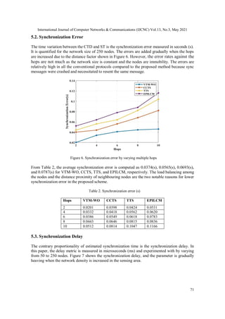
4.4. Synchronization Error Minimization using Whale Optimization
Optimization techniques are proved in resolving different issues of network operations. As
synchronization error 𝑆𝑍𝑒 is constantly challenging in the existing synchronization protocols, a
recently presented whale optimization algorithm (WOA) is integrated to minimize the errors. The
WOA [33] describes the hunting behaviour of humpback whales for the prey in which three
phases are segmented such as encircling, bubble-net feeding, and searching. In the proposed
VTM-WO, the prey is a sync time, humpback whales are sync errors, and the fitness function F
is to reduce the errors between actual and estimated time variation factors. The CTD, 𝑆𝑍𝑡, and ∞
are assumed as the input to a population of WOA. The fitness value is computed to minimize the
occurring errors while updating the sync time that is given as:
𝐹𝑚𝑖𝑛 =
1
𝑉
∑ |𝐴𝑛 − 𝐸𝑛|
𝑉
𝑛=1 (9)](https://image.slidesharecdn.com/13321cnc04-210630084404/85/Clock-Synchronization-using-Truncated-Mean-and-Whale-Optimization-for-Clustered-Sensor-Networks-10-320.jpg)
![International Journal of Computer Networks & Communications (IJCNC) Vol.13, No.3, May 2021
67
where 𝑉 indicates the total number of nodes, 𝐴 and 𝐸 represents the actual and estimated time of
the message transmission and |𝐴𝑛 − 𝐸𝑛 | is referred to 𝑆𝑍𝑒.
Phase 1: Encircling the prey – The whales commence the hunting process in which the present
location is considered as the best solution or close to the optimum region. After the best position
is identified then, the whales are moving towards it. This performance is applied in VTM-WO as:
The nodes’ current time is a source to compute a sync time and time variations are equalized
when member nodes update the new sync time 𝑆𝑍𝑡 that is considered as the best time in the
network. Such a process is expressed as:
∞ = |𝑋 × 𝑡𝑏(𝑖) − 𝑡(𝑖)| (10)
𝑡(𝑖 + 1) = 𝑡𝑏(𝑖) − 𝑌 × ∞ (11)
where 𝑖 represents the iteration, 𝑡𝑏
defines the best time that requires to be updated in the
network, 𝑡 indicates the current time, 𝑋 and 𝑌 denotes the coefficient vectors that are computed
as:
𝑋 = 2𝑥 × 𝑦 − 𝑥 (12)
𝑌 = 2 × 𝑦 (13)
where 𝑥 is sequentially reduced from 2 to 0 over the periods and 𝑦 represents a random number
in the range [0,1].
Phase 2: Bubble-net attacking behaviour – This is referred to as the exploitation phase that
comprises two imperative mechanisms.
Shrinking encircling prey mechanism: This approach shrinks the sync errors by
reducing the value 𝑥 given in the Eq. (12). Subsequently, 𝑌 also is reduced in the
range [−𝑥, 𝑥] from 2 to 0. The new sync time (𝑡𝑏
and CTD) is defined when the
random values for 𝑌 in [-1,1].
Updating spiral position mechanism: This approach computes the time variation
between 𝑡 (whale position), and 𝑡𝑏
(prey position). The spiral equation between
these two is derived as:
𝑡(𝑖 + 1) = ∞′ × 𝑒𝑝𝑞
× cos(2𝜋𝑞) + 𝑡𝑏(𝑖) (14)
where ∞′ = |𝑡𝑏(𝑖) − 𝑡(𝑖)|, 𝑝 is a constant value for the logarithmic spiral and 𝑞 is a random
number in the interval [-1,1]. We assume that there is a 50% possibility to select any one of the
mechanisms to update the sync time while performing optimization and is formulated as given
below:
𝑡(𝑖 + 1) = {
𝑡𝑏(𝑖) − 𝑌 × ∞ 𝑖𝑓 𝑍 < 0.5
∞′ × 𝑒𝑝𝑞
× cos(2𝜋𝑞) + 𝑡𝑏(𝑖) 𝑖𝑓 𝑍 ≥ 0.5
(15)
where 𝑍 is in [0,1] means, 𝑡𝑏
search for CTD to quantify the synchronization factor ∞𝑛.](https://image.slidesharecdn.com/13321cnc04-210630084404/85/Clock-Synchronization-using-Truncated-Mean-and-Whale-Optimization-for-Clustered-Sensor-Networks-11-320.jpg)
![International Journal of Computer Networks & Communications (IJCNC) Vol.13, No.3, May 2021
68
Phase 3: Search for prey – It is also known as the exploration phase. In the network, nodes are
searching for the best 𝑡𝑏
randomly because the optimal sync time is not known. This phase
exploits the variation of 𝑌 in interval [-1,1] to update the best time in the randomly selected
nodes. These two activities are aiming to minimize the errors that are expressed as:
∞ = |𝑋 × 𝑡𝑟𝑎𝑛𝑑 − 𝑡| (16)
𝑡(𝑖 + 1) = 𝑡𝑟𝑎𝑛𝑑 − 𝑌 × ∞ (17)
The current time of the nodes are randomly chosen from the network population and is
represented as 𝑡𝑟𝑎𝑛𝑑. The fitness function of the WOA algorithm for minimizing synchronization
errors is robust and efficient. Hence, this optimization technique can provide a faster convergence
speed by the low time-variation error factor. The pseudo-code for WOA-based synchronization
error minimization is given as follows:
Pseudo Code 3: WOA-Based Synchronization Error Minimization
1. Start procedure
2. Initialize the input (CTD, 𝑆𝑍𝑡, and ∞) with maximum iterations.
3. Compute the fitness using Eq. (9).
4. 𝑡𝑏
is assumed as the best time.
5. while (𝑖 < max_iteration)
6. for each 𝑛 do
7. Update 𝑥, 𝑋, 𝑌, 𝑞, 𝑍
8. if (𝑍 < 0.5) then
9. if (𝑌 < 1) then
10. Execute the Eq. (10).
11. else if (𝑌 >=1) then
12. Select a search node randomly (𝑡𝑟𝑎𝑛𝑑)
13. Execute the Eq. (17).
14. end if
15. else if (𝑍 >= 0.5) then
16. Execute the Eq. (14).
17. end if
18. end for
19. end while
20. return 𝑡𝑏
21. End procedure
4.5. Average Synchronization Error Analysis
Typically, a message transmission through multiple intermediate nodes would persuade the delay
error due to the propagation time component in particular. The timestamp CTD is a vital
parameter to compute the 𝑆𝑍𝑒. The arrival time of a sync_pack and the expected time of delivery
may cause the time variation during the synchronization in the proposed VTM-WO protocol.
Therefore, it is important to analyse the time utilized to calculate and update the sync time among
the nodes. Let assume a cluster consists of 𝑆 nodes for intra-cluster and 𝑘 cluster heads for inter-
cluster that are required to sync with 𝑆𝑍𝑡′ and 𝑆𝑍𝑡′′ respectively, in the network. The average of](https://image.slidesharecdn.com/13321cnc04-210630084404/85/Clock-Synchronization-using-Truncated-Mean-and-Whale-Optimization-for-Clustered-Sensor-Networks-12-320.jpg)
![International Journal of Computer Networks & Communications (IJCNC) Vol.13, No.3, May 2021
69
the relative clock for intra-cluster 𝑆𝑍𝑒′ and inter-cluster 𝑆𝑍𝑒′′ synchronization errors are as
follows:
𝑆𝑍𝑒′ = ∫
[𝐶𝑛(𝑡)−𝐶(𝑡)]
𝑆
𝑆
𝑛=1
(18)
𝑆𝑍𝑒′′ = ∫
[𝐶ℎ(𝑡)−𝐶(𝑡)]
𝑘
𝑘
ℎ=1
(19)
where 𝐶𝑛(𝑡), 𝐶ℎ(𝑡) are defined in Eq. (2), and 𝐶(𝑡) is given in Eq. (1). When a head node ℎ and
BS initiates the sync process, the multi-hop VTM-WO protocol repeats a sync_message
transmission till the process is completed.
𝑆𝑍𝑒′ = ∫
[∞𝑛((𝜆𝑛+𝛾𝑛𝑡)−𝑆𝑍𝑡′)]𝑖
𝑗
𝑆
𝑆
𝑛=1
(20)
𝑆𝑍𝑒′′ = ∫
[∞ℎ((𝜆ℎ+𝛾ℎ𝑡)−𝑆𝑍𝑡′′)]𝑖
𝑗
𝑘
𝑘
ℎ=1
(21)
The synchronization factor ∞ for both intra and inter is delineated in section 4.4., the sync times
𝑆𝑍𝑡′, 𝑆𝑍𝑡′′ are derived from using Eq. (6) at iteration 𝑖=1 to 𝑗, maximum iteration. The time
variation 𝑡𝑣 is a constant predefined value, magnitude in ∞ and 𝑆𝑍𝑡 when the iteration is ended,
that is given as:
𝑆𝑍𝑒′ = ∫
[
∞𝑛
𝑡𝑣
((𝜆𝑛+𝛾𝑛𝑡)−
𝑆𝑍𝑡′
𝑡𝑣
)]
𝑆
𝑆
𝑛=1
(22)
𝑆𝑍𝑒′′ = ∫
[
∞ℎ
𝑡𝑣
((𝜆ℎ+𝛾ℎ𝑡)−
𝑆𝑍𝑡′′
𝑡𝑣
)]
𝑘
𝑘
ℎ=1
(23)
The 𝜆𝑛 , and 𝜆ℎ are eradicated because their values become 0 once the sync time is computed
hence, it is defined as 𝑆𝑍𝑡 = 𝛾𝑡 × ∞. This activity is applied in Eq. (22) and Eq. (23) then, we
obtain
𝑆𝑍𝑒′ = ∫
[
∞𝑛
𝑡𝑣
((𝛾𝑛𝑡)−
𝛾𝑛𝑡×∞𝑛
𝑡𝑣
)]
𝑆
𝑆
𝑛=1
(24)
𝑆𝑍𝑒′′ = ∫
[
∞ℎ
𝑡𝑣
((𝛾ℎ𝑡)−
𝛾ℎ𝑡×∞ℎ
𝑡𝑣
)]
𝑘
𝑘
ℎ=1
(25)
The sync factor value is rounded off to a certain fractional point and is estimated by:
𝑆𝑍𝑒′ = ∫
𝛾𝑛𝑡 [
∞𝑛
𝑡𝑣
−
∞𝑛
𝑡𝑣
]
𝑆
𝑆
𝑛=1
(26)
𝑆𝑍𝑒′′ = ∫
𝛾ℎ𝑡 [
∞ℎ
𝑡𝑣
−
∞ℎ
𝑡𝑣
]
𝑘
𝑘
ℎ=1
(27)
Hence, the average synchronization errors for intra and inter-cluster synchronizations are 𝑆𝑍𝑒′ ≈
0 and 𝑆𝑍𝑒′′ ≈ 0.](https://image.slidesharecdn.com/13321cnc04-210630084404/85/Clock-Synchronization-using-Truncated-Mean-and-Whale-Optimization-for-Clustered-Sensor-Networks-13-320.jpg)
![International Journal of Computer Networks & Communications (IJCNC) Vol.13, No.3, May 2021
70
5. RESULTS AND OBSERVATIONS
In this section, the proposed VTM-WO has experimented with the standard existing TS protocols
such as CCTS [23], TTS [22], and EPILCM [29] using MATLAB 2016a. The nodes' random
deployment in WSN does not guarantee the complete coverage of the network, and VTM-WO
consists of un-even sized clusters. The performance metrics considered for comparison are clock
offset, clock skew, synchronization error, synchronization delay, communication overhead,
energy consumption, and overall processing time. The results of these metrics are illustrated with
the diagrams in the following subsections. The simulation parameters are depicted in Table 1.
Table 1. Simulation parameters
Parameter Values
Sensing area 250m × 250m
Number of nodes 50, 100, 150, 200, 250
Sink position (BS) 240m × 240m
Transmission range 15m
Deployment of nodes Random
MAC protocol TDMA
5.1. Clock Offset and Skew Convergence
The less count of difference among the node’s local clocks enhances the synchronization
precision. VTM-WO is a master-slave synchronization architecture in which every head node
calculates the offset and skew convergences of member nodes using the CTD method. The
network’s convergence rate increases only if clock offset and skew errors are reduced.
Figure 5 demonstrates the results of the clock offset and skews in nanoseconds (ns) for the 250
nodes’ density. The time over the offset and skew are estimated effectively by utilizing truncated
mean square error. As shown in figure 5.a., the clock offset values are 0.57(ns), 0.68(ns),
0.79(ns), and 0.90(ns) for VTM-WO, CCTS, TTS, and EPILCM, respectively. The variation in
time between the nodes’ clock frequencies is shown in figure 5.b. The skew convergence for the
proposed algorithm is 1.07(ns), and other conventional protocols are 1.50(ns), 2.59(ns), and
3.68(ns). Hence, the convergence is quicker in VTM-WO.
5.a. Offset 5.b. Skew
Figure 5. Clock convergence](https://image.slidesharecdn.com/13321cnc04-210630084404/85/Clock-Synchronization-using-Truncated-Mean-and-Whale-Optimization-for-Clustered-Sensor-Networks-14-320.jpg)
![International Journal of Computer Networks & Communications (IJCNC) Vol.13, No.3, May 2021
73
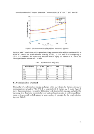
Figure 8. Synchronization messages for different size
All network size together, VTM-WO diminishes the synchronization message overhead by
26.82%, 41.75%, and 49.67% as compared to CCTS, TTS, and EPILCM. This phenomenon
result is reflected in energy dissipation and overall processing time.
Table 4. Communication overhead (Number of messages exchanged)
Network Size VTM-WO CCTS TTS EPILCM
50 57 153 332 481
100 158 316 466 589
150 382 497 591 622
200 491 582 616 709
250 519 648 754 792
5.5. Energy Consumption
The energy depletion is computed by the mathematical derivations discussed in [10]. Figure 9
obtains the energy usage for different sizes during synchronization in which the power dissipation
is increased exponentially between 200 and 250 nodes due to communication overhead. It is
observed that when the network size is enlarged then the involvement of transmitters and
receivers is also increased which led to more energy dissipation. The proposed method dissipates
less energy due to the minimized synchronization of message exchanges at all the network sizes.
For example, at network size 150, VTM-WO consumed 0.2777(J) whereas 0.7359(J), 0.7847(J),
and 0.9374(J) by CCTS, TTS, and EPILCM, respectively.](https://image.slidesharecdn.com/13321cnc04-210630084404/85/Clock-Synchronization-using-Truncated-Mean-and-Whale-Optimization-for-Clustered-Sensor-Networks-17-320.jpg)
![International Journal of Computer Networks & Communications (IJCNC) Vol.13, No.3, May 2021
75
6. CONCLUSIONS AND FUTURE WORK
The proposed VTM-WO achieves the sender-to-receiver synchronization among the nodes in the
clusters. The protocol incorporates the REEC non-overlap clustering to actualize the entire
homogeneous network as energy-efficient. The CTD variations in both intra-cluster and inter-
cluster synchronizations are compensated with a standard time using the truncated mean function.
Also, the synchronization factor between 𝐶𝑛(𝑡) and 𝑆𝑍𝑡 is carried out in less error by the whale
optimization's fitness function. The proposed work has been evaluated and compared with CCTS,
TTS, and EPILCM. Simulation results show that the clock offset and skew errors are minimized
in VTM-WO than the conventional protocols. Further, multi-hop message exchanges are attained
at a lesser hop count that reduces the message transmission overhead. The experimental outcomes
demonstrate that the proposed protocol synchronizes the local clocks with the least amount of
delay and power consumption in the network. The overall performance of VTM-WO is highly
improved where can implement in many applications of WSNs. However, the proposed scheme
has some limitations such as the synchronization delay increases abruptly due to multiple
message exchanges when the network size is augmented, and the nodes' energy is decreased
rapidly if the transmission range is high. The future work will be focused on dynamic cluster
topology with the resynchronization loop for the heterogeneous network considering the delay
parameter.
CONFLICTS OF INTEREST
The authors declare no conflict of interest.
REFERENCES
[1] B. Sundararaman et al., (2005) “Clock synchronization for wireless sensor networks: a survey”, Ad
Hoc Networks, Vol. 3, No. 3, pp. 281-323.
[2] M. Xu, et al., (2016) “Energy-efficient time synchronization in wireless sensor networks via
temperature-aware compensation”, ACM Transactions on Sensor Networks, Vol. 12, No. 2, pp. 1-29.
[3] K. S. Yildirim, (2016) “Gradient descent algorithm inspired adaptive time synchronization in
wireless sensor networks”, IEEE Sensors Journal, Vol. 16, No. 13, pp. 5463-5470.
[4] Z. Wang, et al., (2017) “Cluster-based maximum consensus time synchronization for industrial
wireless sensor networks”, Sensors, Vol. 17, pp. 1-16, doi:10.3390/s17010141.
[5] J. He, et al., (2013) “Time synchronization in WSNs: A maximum-value-based consensus approach”,
IEEE Transactions on Automatic Control, Vol. 59, No. 3, pp. 660-675.
[6] Y. R. Faizulkhakov, (2007) “Time synchronization methods for wireless sensor networks: A survey”,
Programming and Computer Software, Vol. 33, No. 4, pp. 214–226.
[7] J. Li, et al., (2016) “Efficient time synchronization for structural health monitoring using wireless
smart sensor networks”, Structural Control and Health Monitoring, Vol. 23, No. 3, pp. 470-486.
[8] N. Sangjumpa, et al., (2016) “Analysis of adaptive multi-hop time synchronization in large wireless
sensor networks”, 7th International Conference of Information and Communication Technology for
Embedded Systems (IC-ICTES), Bangkok, Thailand, pp. 79-84,
doi:10.1109/ICTEmSys.2016.7467126.
[9] Z. G. Al-Mekhlafi, et al., (2019) “Firefly-inspired time synchronization mechanism for self-
organizing energy-efficient wireless sensor networks: A survey”, IEEE Access, Vol. 7, pp. 115229-
115248.
[10] S. Karthik, & A. Ashok Kumar, (2020) “Ratings based energy-efficient clustering protocol for multi-
hop routing in homogeneous sensor networks”, International Journal of Intelligent Engineering and
Systems, Vol. 13, No. 3, pp. 304-314.
[11] M. Xu, et al., (2014) “A Cluster-based secure synchronization protocol for underwater wireless
sensor networks”, International Journal of Distributed Sensor Networks, Vol 10, No. 4, pp. 1-13.
[12] M. Elsharief, et al., (2018) “FADS: Fast scheduling and accurate drift compensation for time
synchronization of wireless sensor networks”, IEEE Access, Vol. 6, pp. 65507-65520.](https://image.slidesharecdn.com/13321cnc04-210630084404/85/Clock-Synchronization-using-Truncated-Mean-and-Whale-Optimization-for-Clustered-Sensor-Networks-19-320.jpg)
![International Journal of Computer Networks & Communications (IJCNC) Vol.13, No.3, May 2021
76
[13] Y. P. Tian, et al., (2020) “Delay compensation-based time synchronization under random delays:
Algorithm and Experiment”, IEEE Transactions on Control Systems Technology, pp.1-16,
doi:10.1109/TCST.2019.2956031.
[14] Z. Liu, et al., (2018) “Access control model based on time synchronization trust in wireless sensor
networks”, Sensors, Vol. 18, No. 7, pp. 1-15.
[15] J. He, et al., (2017) “Accurate clock synchronization in wireless sensor networks with bounded
noise”, Automatica, Vol. 81, pp. 350–358.
[16] Y. –P. Tian, et al., (2016) “Structural modeling and convergence analysis of consensus-based time
synchronization algorithms over networks: Non-topological conditions”, Automatica, Vol. 65, pp.
64–75.
[17] X. Zhang et al., (2019) “RMTS: A robust clock synchronization scheme for wireless sensor
networks”, Journal of Network and Computer Applications, Vol. 135, pp. 1-10.
[18] X. Sun, X., et al., (2019) “Photovoltaic modules monitoring based on WSN with improved time
synchronization”, IEEE Access, Vol. 7, pp. 132406-132412.
[19] T. Qiu, et al., (2017) “SRTS: A self-recoverable time synchronization for sensor networks of
healthcare IoT”, Computer Networks, Vol. 129, pp. 481-492.
[20] D. Djenouri, et al., (2013) “Fast distributed multi-hop relative time synchronization protocol and
estimators for wireless sensor networks”, Ad Hoc Networks, Vol. 11, No. 8, pp. 2329–2344.
[21] S. Karthik, & A. Ashok Kumar, (2015) “A constructive analysis of time synchronization in wireless
sensor networks”, International Journal of Computer Science and Technology, Vol. 6, No. 3, pp. 56-
60.
[22] J. Wang, et al., (2014) “Two-hop time synchronization protocol for sensor networks”, EURASIP
Journal on Wireless Communications and Networking, Vol. 39, pp. 1-10, doi:10.1186/1687-1499-
2014-39.
[23] J. Wu, et al., (2015) “Cluster-based consensus time synchronization for wireless sensor networks”,
IEEE Sensors Journal, Vol. 15, No. 3, pp. 1404–1413.
[24] F. Shi, et al., (2019) “Novel maximum likelihood estimation of clock skew in one-way broadcast time
synchronization”, IEEE Transactions on Industrial Electronics, Vol. 67, No. 11, pp. 9948-9957.
[25] H. Yan, et al., (2017) “Dynamic adjusting time synchronization for sensor networks”, International
Conference on Computer, Information and Telecommunication Systems (CITS), Dalian, China,
doi:10.1109/CITS.2017.8035324.
[26] H. Wang, et al., (2017) “Estimation of frequency offset for time synchronization with immediate
clock adjustment in multihop wireless sensor networks”, IEEE Internet of Things Journal, Vol. 4, No.
6, pp. 2239-2246.
[27] F. Nunez, et al., (2017) “Pulse-coupled time synchronization for distributed acoustic event detection
using wireless sensor networks”, Control Engineering Practice, Vol. 60, pp. 106-117.
[28] N. Panigrahi, & P.M. Khilar, (2017) “Multi-hop consensus time synchronization algorithm for sparse
wireless sensor network: A distributed constraint-based dynamic programming approach”, Ad Hoc
Networks, Vol. 61, pp. 124-138.
[29] M. Muthumalathi, et al., (2019) “Efficient clock synchronization using energy based proportional
integral and least common multiple protocol in wireless sensor networks”, Journal of Engineering
Science and Technology Review, Vol. 12, No. 4, pp. 144-151.
[30] G. S. S. Chalapathi, et al., (2019) “E-SATS: An efficient and simple time synchronization protocol
for cluster-based wireless sensor networks”, IEEE Sensors Journal, Vol. 19, No. 21, pp. 10144-
10156.
[31] D. Upadhyay, & A. K. Dubey, (2020) “Maximum probable clock offset estimation (MPCOE) to
reduce time synchronization problems in wireless sensor networks”, Wireless Personal
Communications, Vol. 114, No. 2, pp. 1177-1190.
[32] W. Heinzelman, et al., (2002) “An application-specific protocol architecture for wireless micro sensor
networks”, IEEE Transactions on Wireless Communications. Vol. 1, No. 4, pp. 660-670.
[33] S. Mirjalili, & A. Lewis, (2016) “The Whale Optimization Algorithm”, Advances in Engineering
Software, Vol. 95, pp. 51–67.](https://image.slidesharecdn.com/13321cnc04-210630084404/85/Clock-Synchronization-using-Truncated-Mean-and-Whale-Optimization-for-Clustered-Sensor-Networks-20-320.jpg)


![[IJET-V1I3P13] Authors :Aishwarya Manjunath, Shreenath K N, Dr. Srinivasa K G.](https://cdn.slidesharecdn.com/ss_thumbnails/ijet-v1i3p13-150618142708-lva1-app6892-thumbnail.jpg?width=640&height=640&fit=bounds)