Classification Models Machine Learning.pptx

Evaluation of Classification
Models

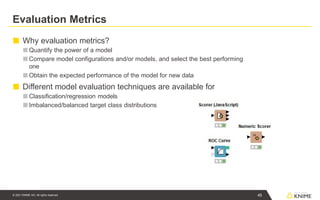
Evaluation Metrics
■ Why evaluation metrics?
■ Quantify the power of a model
■ Compare model configurations and/or models, and select the best performing
one
■ Obtain the expected performance of the model for new data
■ Different model evaluation techniques are available for
■ Classification/regression models
■ Imbalanced/balanced target class distributions
45
© 2021 KNIME AG. All rights reserved.

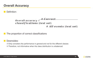
Overall Accuracy
■ Definition:
𝑶𝒗𝒆𝒓𝒂𝒍𝒍 𝒂𝒄𝒄𝒖𝒓𝒂𝒄𝒚 =
# 𝑪𝒐𝒓𝒓𝒆𝒄𝒕
𝒄𝒍𝒂𝒔𝒔𝒊𝒇𝒊𝒄𝒂𝒕𝒊𝒐𝒏𝒔 (𝒕𝒆𝒔𝒕 𝒔𝒆𝒕)
# 𝑨𝒍𝒍 𝒆𝒗𝒆𝒏𝒕𝒔 (𝒕𝒆𝒔𝒕 𝒔𝒆𝒕)
■ The proportion of correct classifications
■ Downsides:
■ Only considers the performance in general and not for the different classes
■ Therefore, not informative when the class distribution is unbalanced
46

Confusion Matrix for Sailing Example
47
■ Rows – true class values
■ Columns – predicted class values
■ Numbers on main diagonal – correctly classified samples
■ Numbers off the main diagonal – misclassified samples
Sailing
yes / no
Predicted
class: yes
Predicted
class: no
True class:
yes
22 3
True class:
no
12 328
Sailing
yes / no
Predicted
class: yes
Predicted
class: no
True class:
yes
0 25
True class:
no
0 340
*,+
Ac𝑐𝑢𝑟𝑎𝑐𝑦 = *+#
=
0,96
*,+
Ac𝑐𝑢𝑟𝑎𝑐𝑦 = * - #
=
0,93

Confusion Matrix
48
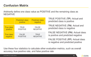
Arbitrarily define one class value as POSITIVE and the remaining class as
NEGATIVE
TRUE POSITIVE (TP): Actual and
predicted class is positive
TRUE NEGATIVE (TN): Actual and
predicted class is negative
FALSE NEGATIVE (FN): Actual class
is positive and predicted negative
FALSE POSITIVE (FP): Actual class
is negative and predicted positive
Use these four statistics to calculate other evaluation metrics, such as overall
accuracy, true positive rate, and false positive rate
Predicted class
positive
Predicted class
negative
True class
positive
TRUE
POSITIVE
FALSE
NEGATIVE
True class
negative
FALSE
POSITIVE
TRUE
NEGATIVE

ROC Curve
■ The ROC Curve shows the false positive rate and true positive rate for
different threshold values
■ False positive rate (FPR)
■ negative events incorrectly classified as positive
■ True positive rate (TPR)
■ positive events correctly classified as positive
Optimal
threshold
Predicted
class positive
Predicted class
negative
True
class
positive
True Positive
(TP)
False Negative
(FN)
True
class
negative
False
Positive (FP)
True Negative
(TN)
𝑇𝑃𝑅
=
𝑇𝑃
𝑇𝑃
+ 𝐹𝑁
𝐹𝑃𝑅
=
𝐹
𝑃
𝐹𝑃
+ 𝑇𝑁
49

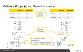
Cohen‘s Kappa (κ) vs. Overall accuracy
Overall
accuracy
�
�
' ! =
19
×
20
100
100
�
�
' $ =
81
×
80
100
100
𝑝' = 𝑝' ! + 𝑝' $ =
0.686
-
10
0
𝑝 =
89
=
0.89
𝜅
= ; : 9
"
9 ! : 9 " #.
%#-
= # . * ; -
≈
0.65
�
�
' ! =
11
×
20
100
100
𝑝' $
=
×
89
80
100
100
𝑝' = 𝑝' ! + 𝑝' $ =
0.734
-
10
0
𝑝 =
81
=
0.81
𝜅
=
! "
=
9 : 9
#.#?,
; : 9 " #.
%,,
=
0.29
Switch TP
and FP
κ = 1: perfect model
performance
κ = 0: the model performance
is equal to a random classifier
50
Positive Negative
Positive 14 6
Negative 5 75
Positive Negative
Positive 6 14
Negative 5 75

Exercise: 01_Training_a_Decision_Tree_Model
51
■ Dataset: Sales data of individual residential properties in Ames, Iowa from 2006
to 2010.
■ One of the columns is the overall condition ranking, with values between 1 and
10.
■ Goal: train a binary classification model, which can predict whether the overall
condition is high or low.
You can download the training workflows from the KNIME
Hub:
https://hub.knime.com/knime/spaces/Education/latest/Courses/

Exercise Session 1
1. Right click on
LOCAL and
select
Import KNIME
Workflow….
■ Import the course material to KNIME Analytics Platform
2. Click on Browse and
select downloaded .knar
file
3. Click on Finish
52

Exercise: Decision_Tree
53

Session II: Regression
Models, Ensemble Models
& Logistic Regression

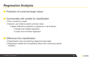
Regression Analysis
56
■ Prediction of numerical target values
■ Commonality with models for classification
■ First, construct a model
■ Second, use model to predict unknown value
■ Major method for prediction is regression in all its flavors
■ Simple and multiple regression
■ Linear and non-linear regression
■ Difference from classification
■ Classification aims at predicting categorical class label
■ Regression models aim at predicting values from continuous-valued
functions

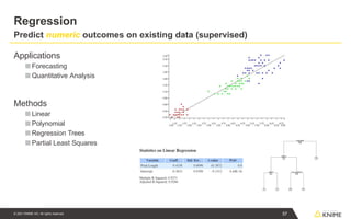
Regression
Predict numeric outcomes on existing data (supervised)
Applications
■ Forecasting
■ Quantitative Analysis
Methods
■ Linear
■ Polynomial
■ Regression Trees
■ Partial Least Squares
57

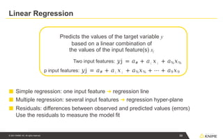
Linear Regression
Predicts the values of the target variable y
based on a linear combination of
the values of the input feature(s) xj
Two input features: 𝑦j = 𝑎# + 𝑎; 𝑥; + 𝑎%𝑥%
p input features: 𝑦j = 𝑎# + 𝑎; 𝑥; + 𝑎%𝑥% + ⋯ + 𝑎9𝑥9
■ Simple regression: one input feature ➔ regression line
■ Multiple regression: several input features ➔ regression hyper-plane
■ Residuals: differences between observed and predicted values (errors)
Use the residuals to measure the model fit
59

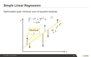
Simple Linear Regression
Optimization goal: minimize sum of squared residuals
x
y
𝑦j
=
𝑎
#
+
𝑎;
𝑥
Residual
ei
∑
$
! " ; ! ! " ;
𝑒%
= ∑$
𝑦!
− 𝑦m!
60
%
yi

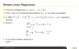
Simple Linear Regression
! " ; ! " ;
■ Think of a straight line 𝑦j = 𝑓 𝑥 = 𝑎 + 𝑏𝑥
■ Find 𝑎 and 𝑏 to model all observations (𝑥!, 𝑦!) as close as possible
■ ➔ SSE 𝐹 𝑎, 𝑏 = ∑$
(𝑓 𝑥 − 𝑦!)% = ∑$
(𝑎 + 𝑏𝑥! − 𝑦!)% should be
minimal
■ That is:
𝜕
𝑎
! " ;
$
!
!
𝜕𝐹
= p 2 𝑎 + 𝑏𝑥 − 𝑦
= 0
𝜕
𝑏
! " ;
$
𝜕𝐹
= p 2 𝑎 + 𝑏𝑥
− 𝑦
61
! !
!
𝑥 =
0
■ ➔ A unique solution exists for 𝑎
and 𝑏

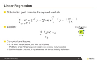
Linear Regression
■ Optimization goal: minimize the squared residuals
■ Solution:
■ Computational issues:
■ 𝑋=𝑋 must have full rank, and thus be invertible
(Problems arise if linear dependencies between input features exist)
■ Solution may be unstable, if input features are almost linearly dependent
∑
$
! " ; ! ! " ; ! @"# @
@,!
%
=
𝑒% = ∑$
𝑦 − ∑$
𝑎 𝑥 𝑦 −
𝑎𝑋 B
𝑦 −
𝑎𝑋
𝑎j
=
𝑋B𝑋 : ; 𝑋
B 𝑦
62

Linear Regression: Summary
63
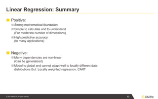
■ Positive:
■ Strong mathematical foundation
■Simple to calculate and to understand
(For moderate number of dimensions)
■High predictive accuracy
(In many applications)
■ Negative:
■Many dependencies are non-linear
(Can be generalized)
■Model is global and cannot adapt well to locally different data
distributions But: Locally weighted regression, CART

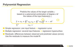
Polynomial Regression
Predicts the values of the target variable y
based on a polynomial combination of degree d of
the values of the input feature(s) xj
■ Simple regression: one input feature ➔ regression curve
■ Multiple regression: several input features ➔ regression hypersurface
■ Residuals: differences between observed and predicted values (errors)
Use the residuals to measure the model fit
@"
;
@"
;
@"
;
ỹ = 𝑎# + ∑9
𝑎@
,
%𝑥%
+ ⋯ +
∑9
@
@
𝑎@,;𝑥@ + ∑9
𝑎@,'𝑥'
64

Evaluation of Regression Models

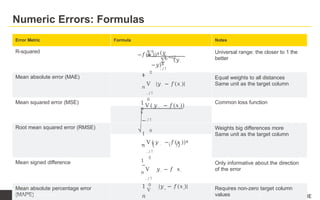
Numeric Errors: Formulas
Error Metric Formula Notes
R-squared ∑0
(𝑦.
−𝑓(𝑥.))$
1 −
. / !
∑0 (𝑦.
−𝑦)$
. / !
Universal range: the closer to 1 the
better
Mean absolute error (MAE) 1
0
𝑛
V |𝑦. − 𝑓(𝑥.)|
. / !
Equal weights to all distances
Same unit as the target column
Mean squared error (MSE)
0
1
𝑛
V ( 𝑦 . − 𝑓(𝑥.))
$
. / !
Common loss function
Root mean squared error (RMSE)
1
0
𝑛
V ( 𝑦 . − 𝑓(𝑥.))$
. / !
Weights big differences more
Same unit as the target column
Mean signed difference 1
0
𝑛
V 𝑦. − 𝑓 𝑥.
. / !
Only informative about the direction
of the error
Mean absolute percentage error
(MAPE)
0
1
V
|𝑦. − 𝑓(𝑥.)|
𝑛
Requires non-zero target column
values 67

MAE (Mean Absolute Error) vs. RMSE (Root Mean Squared Error)
MAE RMSE
Easy to interpret – mean absolute error Cannot be directly interpreted as the average error
All errors are equally weighted Larger errors are weighted more
Generally smaller than RMSE Ideal when large deviations need to be avoided
MAE RMSE
Case 1 2.25 2.29
Case 2 3.25 3.64
Example:
Actual values = [2,4,5,8],
Case 1: Predicted Values = [4, 6, 8, 10]
68

R-squared vs. RMSE
R-squared RMSE
Relative measure:
Proportion of variability explained by the model
Absolute measure:
How much deviation at each point
Range: Usually between 0 and 1.
0 = no variability explained
1 = all variability explained
Same scale as the target
R-sq RMSE
Case 1 0.96 1.12
Case 2 0.65 1.32
Example:
Actual values = [2,4,5,8],
69

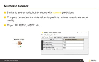
Numeric Scorer
■ Similar to scorer node, but for nodes with numeric predictions
■ Compare dependent variable values to predicted values to evaluate model
quality.
■ Report R2, RMSE, MAPE, etc.
70

Classification Models Machine Learning.pptx

More Related Content

Similar to Classification Models Machine Learning.pptx

Recently uploaded

Classification Models Machine Learning.pptx