Chapter 2 Solving Linear Algebra

1. Chapter 2:
Solving Linear System

2. Learning
Objectives
● At the end of the chapter, we
will be able to:
● 1. Find row echelon form and
reduced row echelon form;
● 2. Solve linear systems using
gauss jordan reduction and
gaussian elimination

3. Learning
Objectives
● 3. Find the inverse of matrix
● 4. Determine the equivalent
matrices
● 5. Discuss the variant of gaussian
elimination which is LU-
Factorization.

4. Table of contents
Row Echelon
Form
2.1
Solving Linear
Systems
2.2
Elementary Matrices;
Finding
2.3
Equivalent Matrices
2.4 2.5
LU
Factorizatio
n

5. ENCHELON FORM OF A
MATRIX
2.1

6. CREDITS: This presentation template was created by Slidesgo
, including icons by Flaticon, infographics & images by
Freepik
An m x n matrix A is said to be in reduced row echelon
from if it satisfies the following properties:
 All zero rows if there are any appear at the bottom of
the matrix.
 The first nonzero entry from the left of a nonzero row is
a 1. This entry is called a leading one of its rows.
 For each nonzero row, the leading one appears to the
right and below any leading ones in preceding rows.
 If a column contains a leading one, then all other
entries in that column are zero.

7. An m x n matrix satisfying properties (a) (b)
and (c) is said to be in row echelon
form.
EXAMPLE:

8. CREDITS: This presentation template was created by Slidesgo
, including icons by Flaticon, infographics & images by
Freepik
An elementary row (column) operation on a Matrix
A is any one of the following operations:
Type I: Interchange any two rows (column).
Ex. R1↔R3
Type II: Multiply row (column) by nonzero
number.
Ex. -3R2→R2
Type III: Add and multiply of one row (column) to
another.
Ex. -3R2 + R4→R4

9. Example 1
Find a row echelon form of each of the given
matrices record the row operations you perform
using the notation for elementary row operations.

10. SOLUTION:

11. Example 2
Find the reduced row echelon form of each of the
given matrices. Record the row operations you
perform, using the notation for elementary row
operations.

12. SOLUTION:

13. Example 3
Find a row echelon form and reduced row echelon
form of the given matrices. Record the row
operations you perform using the notation for
elementary row operations.

14. SOLUTION:
൥
3 3 3
−1 0 −4
2 4 −2
൩ -R2↔R1
൥
1 0 4
3 3 3
2 4 −2
൩ 3R1 + R2 →R2
൥
1 0 4
0 3 −9
2 4 −2
൩ -2R1 + R3 →R3
൥
1 0 4
0 3 −9
0 4 −10
൩ 1
3
R2→R2
൥
1 0 4
0 1 −9
0 4 −10
൩ -4R2 + R3→R3
൥
1 0 4
0 1 −3
0 0 2
൩ 1
2
R3→R3
൥
1 0 4
0 1 −3
0 0 1
൩ 3R3+R2→R2 -row echelon form
൥
1 0 4
0 1 0
0 0 1
൩ -4R3 + R1→R1
൥
1 0 0
0 1 0
0 0 1
൩ Reduced row echelon form

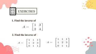
15. EXERCISES
1. Find the reduced row echelon form of each of the given matrices record
the row operation you perform, using the notation for elementary row
operations.
2. Find the row echelon form of each of the given matrices. Record the row
operation you perform, using the notation for elementary row operations.

16. EXERCISES
3. Find the reduce row echelon form of each of the
given matrices. Record the row operation you perform,
using the notation for elementary row operations.

17. SOLVING LINEAR
SYSTEM
2.2

18. Linear equations are equations of the first order.
These equations are defined for lines in the
coordinate system. An equation for a straight line is
called a linear equation. The general representation
of the straight-line equation is y=mx+b, where m is
the slope of the line and b is the y-intercept.
Linear equations are those equations that
are of the first order. These equations are defined for
lines in the coordinate system.

19. The echelon forms are more efficiently in determining
the solution of a linear system compared with the elimination
method. Using the augmented matrix of a linear system
together with an echelon form. we develop two methods for
solving a system of m linear equations in n unknow. These
methods take the augmented matrix of the linear system,
perform elementary row operations on it, and obtain a new
matrix that represents an equivalent linear system. The
important point is that the latter linear system can be solved
more easily.

20. Represents the augmented matrix of a linear system. The n the solution is quickly.
found from the corresponding equations

21. The task of this section is to manipulate the augmented
matrix representing a given linear system into a form from
which the solution can be found more easily. We now
apply row operations to the solution of linear systems.

22. • Theorem 2.3 Let Ax = b and Cx = d be two linear systems each of
m equations in n unknowns. If the augmented matrices [A b] and [C
⁞ ⁞
d] arc row equivalent, then the linear systems are equivalent; that is.
they have the same solutions.
• Proof
•This follows from the definition of row equivalence and from the
fact that the three elementary row operations on the augmented matrix
are the three manipulations on linear systems which yield equivalent
linear systems. We also note that if one system has no solution, then the
other system has no solution.

23. Recall from Section 1.1 that the linear system of the
form:
is called a homogeneous system. We can also write (1) in matrix form as

24. We observe that we have developed the
essential features of two very straight-forward
methods for solving linear systems. The idea
consists of starting with the linear system Ax = b,
then obtaining a partitioned matrix [C d] in either
⁞
row echelon form or reduced row echelon form
that is row equivalent to the augmented matrix [A
b].
⁞

25. The method where [C d] is in row echelon form is called
⁞
Gaussian elimination, the method where [C d] is in reduced row
⁞
echelon form is called Gauss'- Jordan reduction. Strictly speaking,
the original Gauss-Jordan reduction was more along the lines
described in the preceding Remark. The version presented in this
book is more efficient. In actual practice, neither Gaussian
elimination nor Gauss-Jordan reduction is used as much as the
method involving the LU-factorization of A that is discussed in
Section 2.5. However. Gaussian elimination and Gauss-Jordan
reduction are fine for small problems, and we use the latter
heavily in this book.

26. CREDITS: This presentation template was created by Slidesgo
, including icons by Flaticon, infographics & images by
Freepik
Gaussian elimination consists of two steps:
Step 1. The transformation of the augmented
matrix [ A b] to the matrix [ C d] in row echelon
⁞ ⁞
form using elementary row operations.
Step 2. Solution of the linear system
corresponding to the augmented matrix [ C d]
⁞
using back substitution for the case in which A ~ n x
n. and the linear system Ax = h has a unique
solution, the matrix [ C d] has the following form.
⁞

27. Example 1.
The linear system
has the augmented matrix

28. Transforming this matrix to row echelon form, we obtain (verify)
Using back substitution, we now have
Thus, the solution is x = 2, y = -1, z = 3, which is unique.

31. CREDITS: This presentation template was created by Slidesgo
, including icons by Flaticon, infographics & images by
Freepik
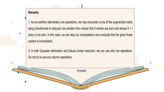
Remarks
1. As we perform elementary row operations, we may encounter a row of the augmented matrix
being transformed to reduced row echelon form whose first II entries are zero and whose II + I
entry is not zero. In this case, we can stop our computations and conclude that the given linear
system is inconsistent.
2. In both Gaussian elimination and Gauss-Jordan reduction, we can use only row operations.
Do not try to use any column operations.

32. 1. Consider the linear system.
x + y +2z= - 1
x – 2y + z = -5
3x+ y + z= 3.
(a) Find all solutions, if any exist. by using the Gaussian
elimination method.
(b) Find all solutions. if any exist. by using the Gauss10rdan reduction method

33. 2. Find an equation relating (a. b. and c so that the linear
system
x + 2-3z = a
2x + 3y + 3z = b
5x + 9y – 6 = c
is consistent for any values of (a, b, and c that satisfy
that equation.

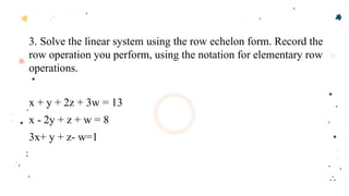
34. 3. Solve the linear system using the row echelon form. Record the
row operation you perform, using the notation for elementary row
operations.
x + y + 2z + 3w = 13
x - 2y + z + w = 8
3x+ y + z- w=1

35. ELEMENTARY MATRICES
FINDING A^-1
2.3

36. • Definition:
An n*n elementary matrix of type
I, type II, or type III is a
matrix obtained from the identity matrix
ln by performing a single elementary
or elementary column operation of type
I, type II, or type III respectively.

37. THEOREM OF ELEMENTARY MATRICES
• Theorem 2.5
Let A be an m*n matrix, and let an elementary row(column) operation of
type I, type II or type III be performed on A to yield matrix B. Let E be the
elementary matrix obtained from lm (ln) by performing the same elementary row
operation as was performed on A. Then B=EA(B=AE).
Example:
• We can readily verify that B= EA

38. Theorem 2.6
If A and B are m*n matrices, then A is
row equivalent to B if and only if there exist
elementary matrices E1,E2,…,Ek such that
B= Ek Ek-1… E2 E1A (B=AE,…E8-1 Ek).
Theorem 2.7
An elementary matrix E is
nonsingular l, and its inverse is an elementary
matrix of the same type.

39. Lemma 2.1
Let A be an n*n matrix and let the homogeneous
system Ax=0 have only the trival solution x=0. Then A is row
equivalent to ln. ( That is the reduced tow echelon form of A is
ln).
Theorem 2.8
A nonsingular if and only if A is a product of
elementary matrices.
Corollary 2.2
A is nonsingular if and only if A is row equivalent to
ln. ( That is the reduced row echelon form of A is ln).

40. Theorem 2.9
The homogeneous system of n linear equations in n unknown
Ax=0 has nontrival solution if and only if A is singular. ( That is, the
reduced row echelon form of A is not equal to ln).
Example:
Consider that homogeneous system Ax=0; that
Let

41. The reduced row
echelon form of
the augmented
Matrix is
(Verify), so a solution is
x= -2r
y= r
Where r is any real number.
Thus the homogeneous system has a nontrivial solution, and A
is singular.

42. Theorem 2.10
An n*n matrix A is singular if and only if A
is row equivalent to matrix B that has a row of zeros
( That is, the reduced row echelon form of A has a
row of zeros).
Theorem 2.11
If A and B are n*n matrices such that
AB=lm, and BA=ln. Thus B A^-1

43. Following are an examples
of Elementary Matrices:

44. EXERCISES
1. Find the inverse of
2. Find the inverse of

45. EXERCISES
3. Determine if the following homogeneous system
has a Nontrivial Solution.
w+2x+3y+2z= 0
w+3x+5y+5z= 0
2w+4x+7y+X= 0
-w-2x-6y+7z= 0

46. EQUIVALENT
MATRICES
2.4

47. We have thus far considered A to be row
(column) equivalent to B if B results from A by
finite sequence of elementary row (column)
operations. A natural extension of this idea is that of
considering B to arise from A by finite sequence of
elementary row (column) operations. This leads to
the notion of equivalence of matrices.

48. If A and B are two m x n matrices, then A is
equivalent to B if we obtain B from A by a finite
sequence of elementary row (column) operations.
A= ቂ
𝑎 𝑐
𝑏 𝑑
ቃ
↶
B= ቂ
𝑎 𝑐
𝑏 𝑑
ቃ

49. I
In the case of row (column) equivalent we can show
that :
A. Every matrix is equivalent to itself
B. If B is equivalent to A, then A is equivalent to
B
C. If C is equivalent to B, and B is equivalent to
A, then C is equivalent to A

50. Let A = Applying elementary row operations, we obtain the
following:
B = A2r3 + r2 → r2 =
C= Br2 ⇔ r3 =

51. D= C2r1 → r1=
So, we show that Matrices A,B,C and D are equivalent by
applying the elementary row operations.. Then, we can also
show that if two matrices are row equivalent, then they are
equivalent.

52. Let A and I be 2x2 matrices defined as
follows :
A= B=
Prove that matrix A is equivalent I

53. A = cr1 – r2 → r2
= 1/cb-d r2
= br2 – r1→ r1
= = I
We can see that we obtain matrix B from A by finite sequence of
elementary row (column) operations.

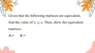
54. Given that the following matrices are equivalent,
find the value of x, y, z. Then, show the equivalent
matrices.
A = b =

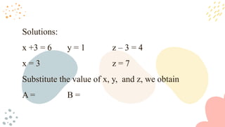
55. Solutions:
x +3 = 6 y = 1 z – 3 = 4
x = 3 z = 7
Substitute the value of x, y, and z, we obtain
A = B =

56. 1. Solve for x, y and z in the Matrix A and B, provided that they are
equivalent
A= B=
2. Given matrix T and Matrix Y, calculate the value of x and y
T = S =
EXERCISES

57. EXERCISES
3. Solve for all variables of the A and B matrix. Then, prove
that they are equivalent.
A = B =

58. LU-Factorization
2.5

59. An LU factorization of an 𝑛𝑥𝑛matrix A is a factorization A= LU, where L is unit lower triangular and U
is upper triangular “Unit” means L has ones on the diagonal.
When U is an upper triangular matrix all of whose diagonal entries are different from zero, then
the linear system 𝑈𝑥= 𝑏can be solve without transforming the augmented matrix [𝑈⁞𝑏] to reduce row
echelon form or to row echelon form. The augmented matrix of such a system is given by
‫ۏ‬
‫ێ‬
‫ێ‬
‫ێ‬
‫ۍ‬
𝑈
11 𝑈
11 𝑈
11 … 𝑈
11 ⁞ 𝑏1
0 𝑈
11 𝑈
11 … 𝑈
11 ⁞ 𝑏2
0 0 𝑈
11 … 𝑈
11 ⁞ 𝑏3
⁞ ⁞ ⁞ … ⁞ ⁞ ⁞
0 0 0 … 𝑈
11 ⁞ 𝑏𝑛 ‫ے‬
‫ۑ‬
‫ۑ‬
‫ۑ‬
‫ې‬

60. The solution is obtained by the following algorithm:
𝑥𝑛 =
𝑏𝑛
𝑈
𝑛𝑛
𝑥𝑛−1 =
𝑏𝑛−1 − 𝑈
𝑛−1 𝑛𝑥𝑛
𝑈
𝑛−1 𝑛−1
⁞
𝑥
𝑗 =
𝑏
𝑗 − σ 𝑈
𝑗 𝑘𝑥𝑘
𝑗−1
𝑘=𝑛
𝑢𝑗𝑗
, j=n ,n-1,…, 2, 1.
This procedure is merely back substitution, which we used in conjunction with Gussian
elimination, in Solving Linear Systems, where it was additionally required that the diagonal entries be 1.

61. In similar manner, if l is a lower triangular matrix all of whose diagonal entries are different from zero,
thelinearsystemLx=bcanbesolvingbyforwardsubstitution,whichconsistsofthefollowingprocedure.
Theaugmentedmatrixhastheform
‫ۏ‬
‫ێ‬
‫ێ‬
‫ێ‬
‫ۍ‬
𝑙11 0 0 … 0 ⁞ 𝑏1
𝑙11 𝑙11 0 … 0 ⁞ 𝑏2
𝑙11 𝑙11 𝑙11 … 0 ⁞ 𝑏3
⁞ ⁞ ⁞ … ⁞ ⁞ ⁞
𝑙11 𝑙11 𝑙11 … 𝑙11 ⁞ 𝑏𝑛 ‫ے‬
‫ۑ‬
‫ۑ‬
‫ۑ‬
‫ې‬

62. And the solution is given by:
𝑥1 =
𝑏1
𝑙11
𝑥2 =
𝑏2 − 𝑙21𝑥1
𝑙22
⁞
𝑥
𝑗 =
𝑏
𝑗 = σ 𝑙𝑗𝑘𝑥𝑘
𝑗−1
𝑘=1
𝑙𝑗𝑗

63. Example 1:
To solve the linear system
5𝑥
1
4𝑥
1 − 2𝑥2
2𝑥
1 + 3𝑥2 + 4𝑥
5𝑥
1 = 10
4𝑥
1 − 2𝑥2 = 28
2𝑥
1 + 3𝑥2 + 4𝑥3 = 26

64. We use forward substitution. Hence we obtain from the previous algorithm
𝑥1 =
10
5
= 2
𝑥2 =
28− 4𝑥1
−2
= −10
𝑥3 =
26− 2𝑥1 − 3𝑥2
4
= 13
Which implies that the solution to the given lower triangular system of equations is
𝑥= ൥
2
−10
13
൩

66. To solve the given system using this LU – factorization, we proceed as follows. Let
൦
2
−4
8
−43
൪
Then we solve Ax=b writing it as Lux=b. First, let Ux=z and use forward substitution solve Lz=b.
‫ۏ‬
‫ێ‬
‫ێ‬
‫ێ‬
‫ۍ‬
1 0 0 0
1
2
1 0 0
−2 −2 1 0
−1 1 −2 1 ‫ے‬
‫ۑ‬
‫ۑ‬
‫ۑ‬
‫ې‬
൦
𝑧
1
𝑧
2
𝑧
3
𝑧
4
൪= ൦
2
−4
8
−43
൪
𝑧
1 = 2

69. Exercises:
1. A= ൥
1 1 1
4 3 −1
3 5 3
൩
,𝑏= ൥
1
6
4
൩
,𝐿= ൥
1 0 0
4 1 0
3 −2 1
൩
,𝑈= ൥
1 1 1
0 −1 −5
0 0 −10
൩
2. 𝐴= ൦
3 −7 −2 2
−3 5 1 0
6 −4 0 −5
−9 5 −5 12
൪, 𝑏= ൦
−9
5
7
11
൪, 𝐿= ൦
1 0 0 0
−1 1 0 0
2 −5 1 0
−3 8 3 1
൪, 𝑈= ൦
3 −7 −2 2
0 −2 −1 2
0 0 −1 1
0 0 0 −1
൪

70. Submitted by Group 2
• Dannazen E. Gullon
• Erica F. Palisoc
• Jhon Lloyd R. Palisoc
• Jessiel P. Quinto
• Elizabeth P. Soriano
• Christine P. Tejada
• Melanie E. Ventura

71. THANK YOU FOR
LISTENING