This document provides an overview of linear algebra, focusing on methods for solving systems of linear equations, including the elimination method, augmented matrices, row echelon form (REF), and reduced row echelon form (RREF). It explains the concepts and applications of these methods, emphasizing Gaussian elimination and Gauss-Jordan elimination techniques used to transform matrices for solving equations. The importance of pivot positions and their roles in matrix transformations is highlighted, along with practical examples and learning outcomes associated with mastering linear algebra.

1. Echelon form and
reduced row echelon
form
L i n e a r A l g e b r a

2. Linear Algebra, a mathematical discipline that deals with vectors and
matrices and, more generally, with vector spaces and linear
transformations. Unlike other parts of mathematics that are frequently
invigorated by new ideas and unsolved problems, linear algebra is very
well understood. Its value lies in its many applications, from
mathematical physics to modern algebra and coding theory.
LINEAR ALGEBRA

3. CONTENT:
1. ELIMINATION METHOD
2. AUGMENTED MATRICES
4. REDUCED ROW ECHELON FORM
3. ROW ECHELON FORM
5. PIVOTS (POSITION & COLUMN)
6. GAUSSIAN ELIMINATION
7. GAUSS-JORDAN ELIMINATION

4. By the end of this lesson, you will be able to:
1. Apply the Elimination Method to solve systems of linear equations.
Learning Objectives
2. Use Augmented Matrices and perform row operations to simplify system
3. Convert Matrices to Row Echelon Form (REF) using Gaussian elimination.
4. Achieve Reduced Row Echelon Form (RREF) using Gauss-Jordan elimination.
5. Identify Pivot Positions and their role in matrix transformations.
6. Solve Systems using matrix methods and interpret solutions efficiently.

5. The elimination method of solving a system of linear equations algebraically is the
most widely used method out of all the methods to solve linear equations. In the
elimination method, we eliminate any one of the variables by using basic arithmetic
operations and then simplify the equation to find the value of the other variable. Then
we can put that value in any of the equations to find the value of the variable
eliminated.
The Elimination Method
As per the elimination method definition, it is about eliminating one of the terms
containing any of the variables to make the calculations easier. This is done by
multiplying or dividing a number by the equation(s) such that the coefficients of any
one of the variable terms become the same. Then, we add or subtract both the
equations to eliminate or remove that term from the result. That is why the elimination
method is also called the addition method.

6. EXAMPLE SYSTEM
Step 1: Add the Equations
Simplify
:
To eliminate y, add the two equations
together:
Step 2: Solve for
x
Step 3: Substitute x=6 into One of the Original Equations
Solve for
y:
Now substitute x=6 into one of the original equations to
find y. We'll use the first equation:
Final
Solution
Step 4: Verify the Solution
Substitute x=6 and y=4 into both original
equations:
For x + y =
10:
For x - y =
2:

7. Solving equations by elimination requires writing the variables x, y, z
and the equals sign = over and over again, merely as placeholders: all that is changing in the
equations is the coefficient numbers. We can make our life easier by extracting only the
numbers, and putting them in a box:
Augmented Matrices and Row Operations
This is called an augmented matrix. The word “augmented” refers to the vertical line, which
we draw to remind ourselves where the equals sign belongs; a matrix or coefficient matrix is a
grid of numbers without the vertical line.

8. In this notation, our three valid ways of manipulating our equations become row operations:
Scaling: multiply all entries in a row by a nonzero number.
Here the notation R1 simply means
“the first row”, and likewise for R2, R3,
etc.
Replacement: add a multiple of one row to another, replacing the second row with the result.
Swap/Interchange: interchange two rows.

9. This lesson introduces the concept of an echelon matrix. Echelon
matrices come in two forms: the row echelon form (REF) and the
reduced row echelon form (RREF).
ECHELON FORM OF A MATRIX

10. ROW ECHELON FORM?
• All nonzero rows are above any rows of all zeros.
A matrix is in row echelon form if it meets the following
conditions:
• Each leading entry of a row is in a column to the right of the leading
• All entries in a column below a leading entry are zeros.

12. EXAMPLES
3x4 matrix in row echelon
form
3x2 matrix in row echelon
form
This matrix is in row echelon form because: This matrix is in Row Echelon Form because:
• All the entries below each leading are
zeros.
• Each leading entry in a row is in a column
to the right of the leading entry of the row
above it, which creates staircase pattern.
• The row with all zeros is positioned at the
bottom
• All the entries below each leading are
zeros.
• The leading entry of row 1 is in column 1,
and the leading entry of row 2 is in column 2,
forming a staircase pattern.

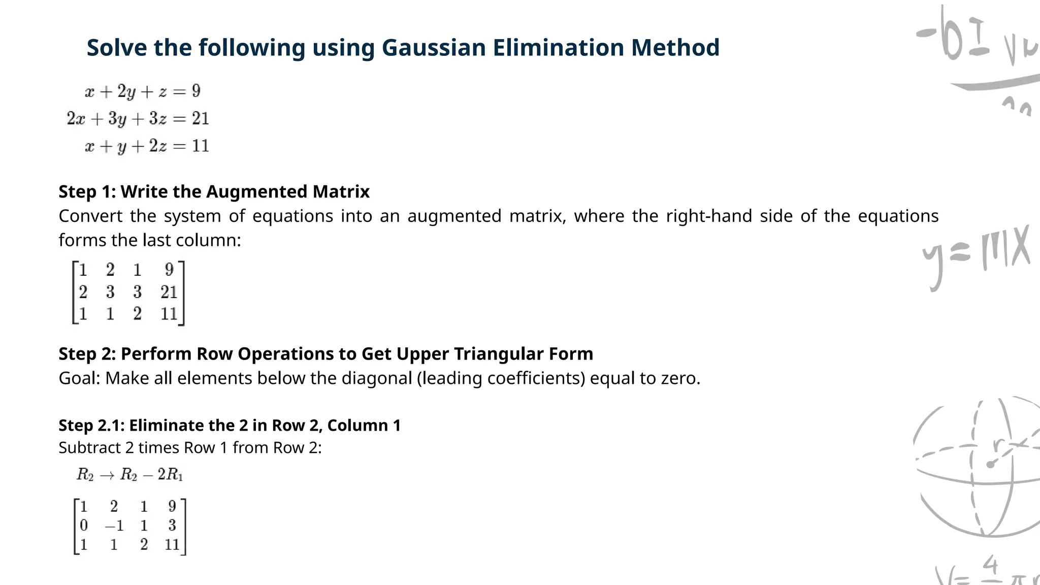
13. STEP 2. Eliminate the leading coefficient in Row 2 by subtracting 2 x Row 1 from Row 2:
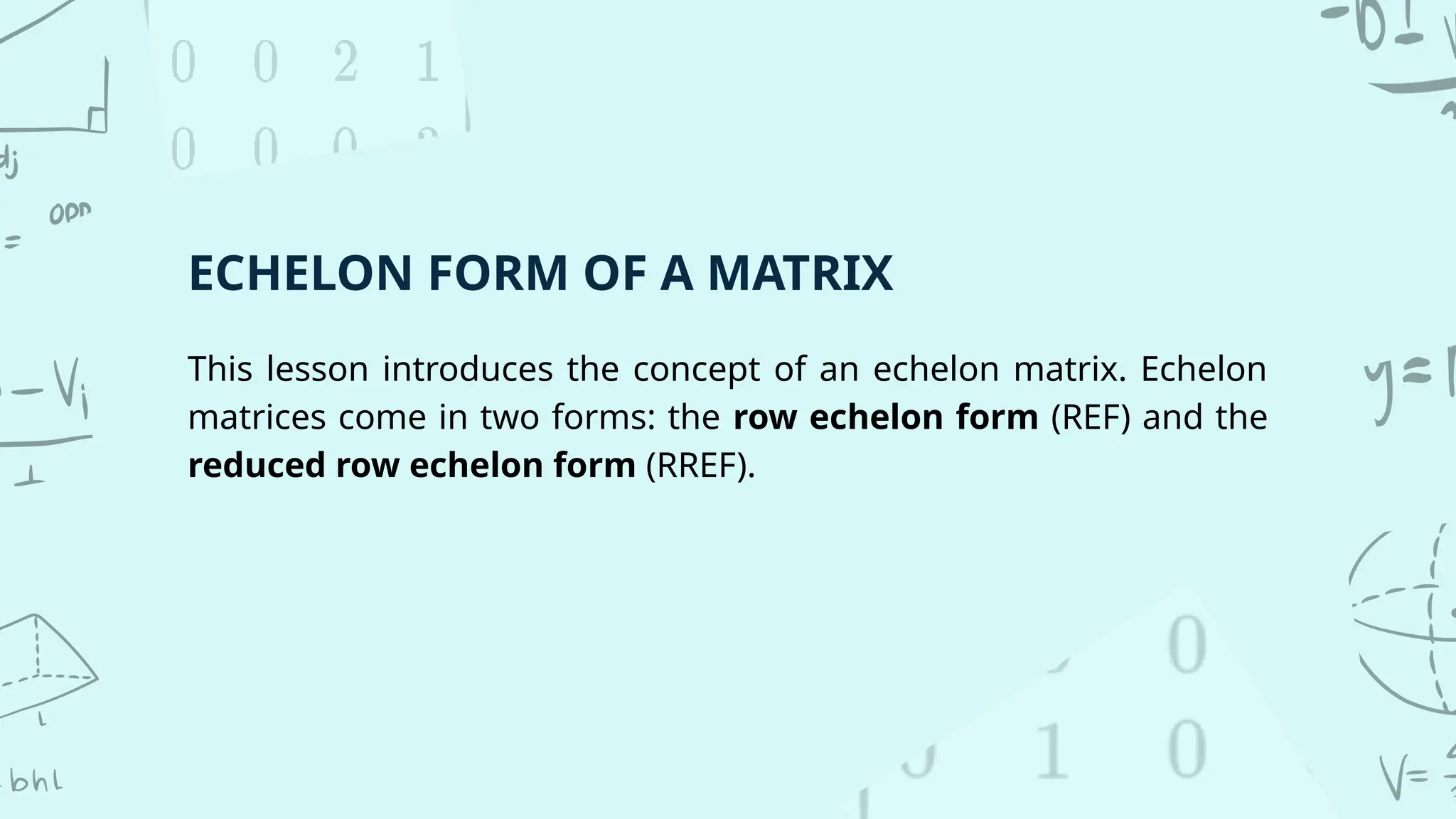
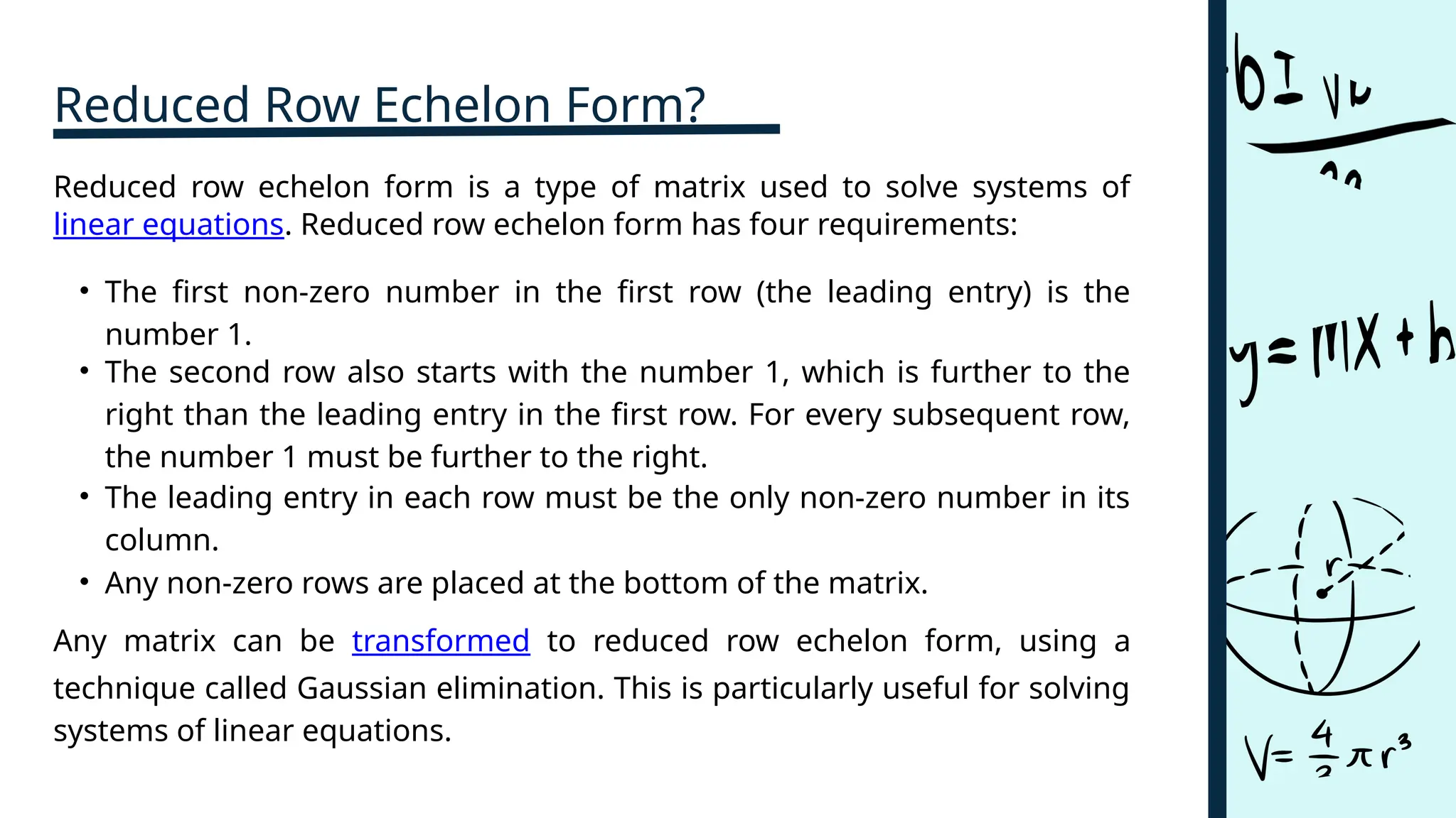
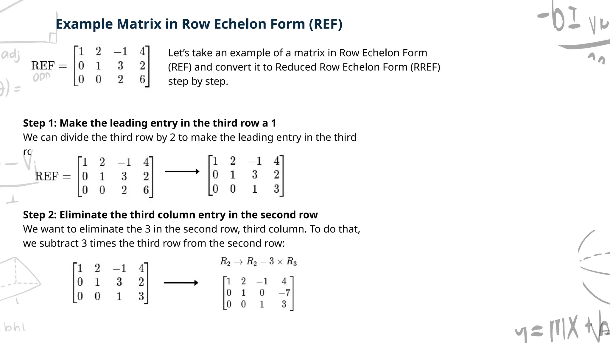
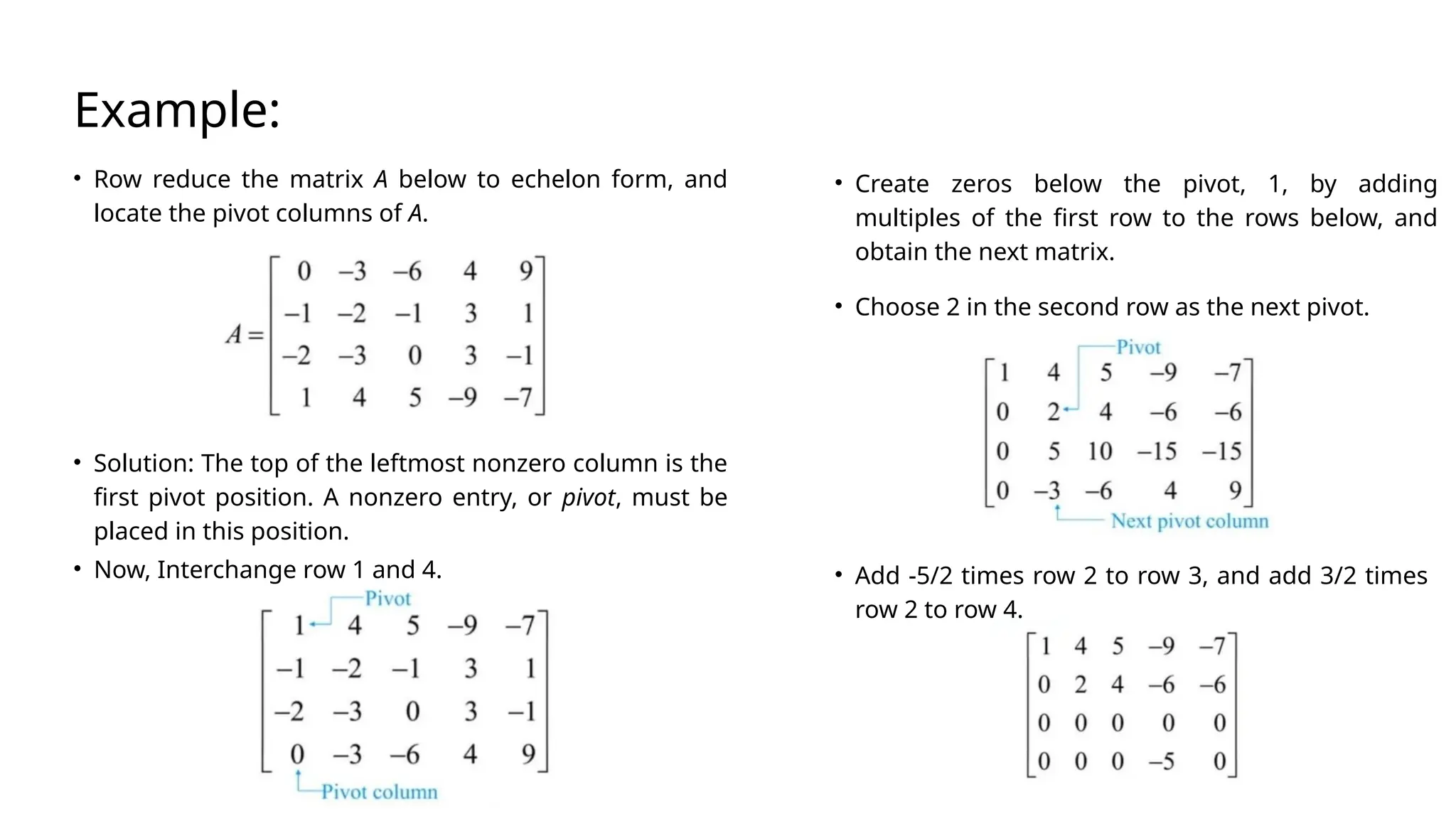
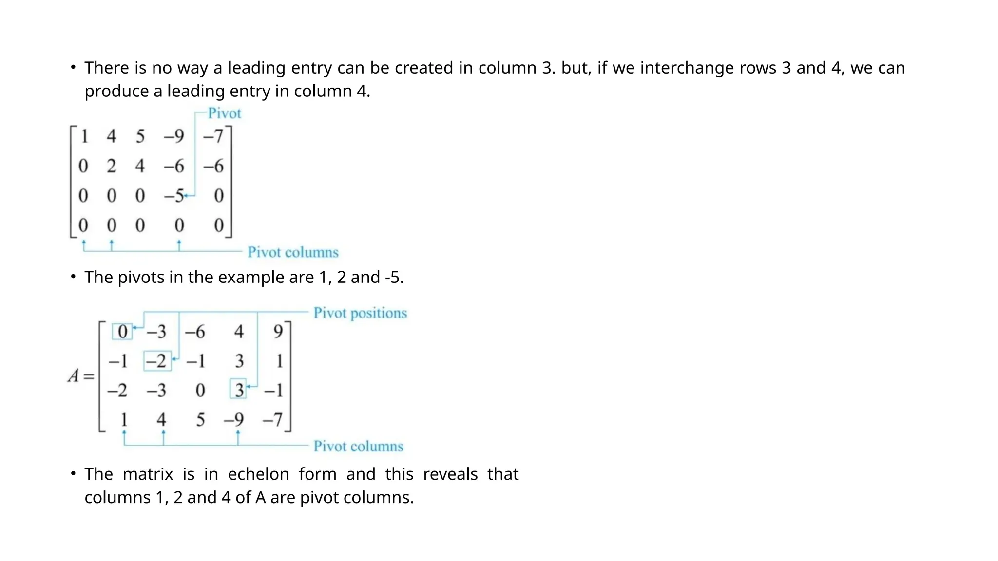
Example of Matrices transforming into Row
Echelon Form (REF)
1.
STEP 1. Swap Row 1 and Row 2 to bring a leading 1 to the
top:
Row 2 Row 2 2×Row 1
→ − ⇒[2 2(1),4 2(2), 2 2(1)]=[0,0, 4]
− − − − −

14. Example of Matrices transforming into Row
Echelon Form (REF)
STEP 3. Eliminate the leading coefficient in Row 3 by subtracting 3×Row 1 from Row 3:
Row 3 Row 3 3×Row 1 [3 3(1),6 3(2),0 3(1)]=[0,0, 3]
→ − ⇒ − − − −
Row 2 1/4​
×Row 2 [0,0,1]
→− ⇒
STEP 4. Scale Row 2 to make the leading entry
1:
STEP 5. Eliminate the entry below Row
2:
Row 3 Row 3+3×Row 2 [0,0, 3+3(1)]=[0,0,0]
→ ⇒ −
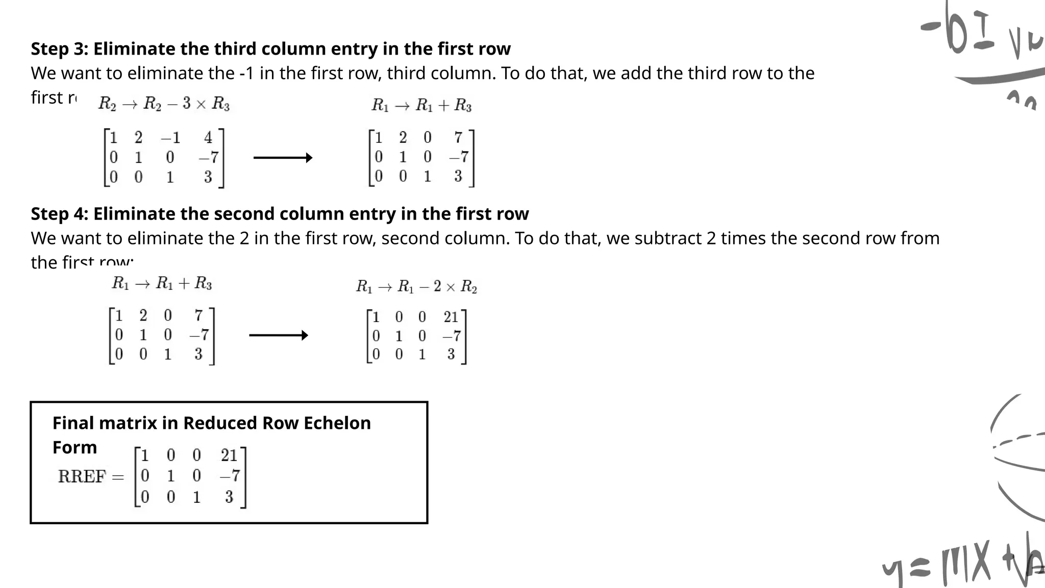
REF=
Final matrix in Row Echelon
Form

15. Example of Matrices transforming into Row
Echelon Form (REF)
2.
STEP 1. Use Row 1 to eliminate leading coefficients in Rows 2 and 3:
For Row 2:
Row 2 Row 2 2×Row 1 [2 2(1),4 2(2),6 2(3)]=[0,0,0]
→ − ⇒ − − −
For Row 3:
Row 3 Row 3 3×Row 1 [3 3(1),6 3(2),9 3(3)]=[0,0,0]
→ − ⇒ − − −
Final matrix of Row Echelon
Form
REF=
This matrix is already in REF, as all non-zero rows
are above any rows of all zeros.

16. Reduced Row Echelon Form?
• The first non-zero number in the first row (the leading entry) is the
number 1.
• The second row also starts with the number 1, which is further to the
right than the leading entry in the first row. For every subsequent row,
the number 1 must be further to the right.
Any matrix can be transformed to reduced row echelon form, using a
technique called Gaussian elimination. This is particularly useful for solving
systems of linear equations.
• Any non-zero rows are placed at the bottom of the matrix.
Reduced row echelon form is a type of matrix used to solve systems of
linear equations. Reduced row echelon form has four requirements:
• The leading entry in each row must be the only non-zero number in its
column.

17. • Asterisks (*) Represent Free Variables:
⚬ The asterisks (*) represent arbitrary entries or
free variables, which could be any value
(including zero). These occur in non-pivot
columns (columns without a leading 1).
⚬ The values in these positions don’t affect the
fact that the matrix is in RREF, but they indicate
flexibility in the solution (free variables).
The matrix is in Reduced Row Echelon Form
because:
• Each row with a non-zero entry starts with a
leading 1.
• The leading 1s move left to right down the
matrix.
• The columns containing the leading 1s are
"clean" with zeros everywhere else in their
respective columns.
• Free Variables and Solutions:
⚬ The columns that do not contain leading 1s
correspond to free variables in the system of
equations.
⚬ The rows with leading 1s correspond to
dependent variables that can be solved in terms
of the free variables.

18. Examples:
• The first two rows each have a leading 1.
Augmented Matrix with a Unique Solution
(3x4)
This could represent a system of linear
equations where:
Rectangular Matrix (3x2)
This matrix is in RREF form because:
• The row below each leading 1 consists
entirely of zeros.
• The final column could be the augmented
part of the matrix, representing the
constants of the system.
• Each row contains a leading 1 with zeros in
all other positions in the column.
• There are three pivot columns.

19. Matrix with a Row of Zeros (4x4)
This matrix has three pivot columns, and the last
row is a zero row. It's still in RREF because:
A Complex 4x5 Matrix (with free
variables)
• The first two rows have leading 1s (pivot
elements) in the first two columns.
• The row of zeros is at the bottom, which is
allowed in RREF.
• The leading 1s move down and to the right.
• The columns with leading 1s have zeros
elsewhere.
• The last row is a zero row, which appears at
the bottom, as required for RREF.
• The third column is a free variable, as there is
no leading 1 in that column.
• The third row has a leading 1 in the fourth
column.

20. Step 1: Make the leading entry in the third row a 1
We can divide the third row by 2 to make the leading entry in the third
row a 1.
Step 2: Eliminate the third column entry in the second row
We want to eliminate the 3 in the second row, third column. To do that,
we subtract 3 times the third row from the second row:
Example Matrix in Row Echelon Form (REF)
Let’s take an example of a matrix in Row Echelon Form
(REF) and convert it to Reduced Row Echelon Form (RREF)
step by step.

21. Step 3: Eliminate the third column entry in the first row
We want to eliminate the -1 in the first row, third column. To do that, we add the third row to the
first row:
Step 4: Eliminate the second column entry in the first row
We want to eliminate the 2 in the first row, second column. To do that, we subtract 2 times the second row from
the first row:
Final matrix in Reduced Row Echelon
Form

22. Pivot position of a matrix?
• refers to a position in a matrix that corresponds to the leading entry
(or the first non-zero entry) in a row after performing Gaussian
elimination (or row-reduction) to transform the matrix into row
echelon form. These pivot positions help identify the basic variables
in a system of linear equations and play a role in solving the system.
• a pivot position of a matrix is any first non-zero term of any non-
zero row.
For instance, in this reduced row echelon matrix,
the pivot positions are indicated in bold:
Pivots

23. Pivot column of a matrix?
• The pivot columns is a column that contains a pivot element. A
pivot element is the first non-zero number in a row when the
matrix is in row echelon form (a form where all the rows below a
pivot are zero).
The matrix is in echelon form and thus
reveals that columns 1, 2, and 4 of A are
pivot columns. The pivots in this example
are 1, 2 and 5.
−
Pivots

24. Example:
• Row reduce the matrix A below to echelon form, and
locate the pivot columns of A.
• Solution: The top of the leftmost nonzero column is the
first pivot position. A nonzero entry, or pivot, must be
placed in this position.
• Now, Interchange row 1 and 4.
• Create zeros below the pivot, 1, by adding
multiples of the first row to the rows below, and
obtain the next matrix.
• Add -5/2 times row 2 to row 3, and add 3/2 times
row 2 to row 4.
• Choose 2 in the second row as the next pivot.

25. • There is no way a leading entry can be created in column 3. but, if we interchange rows 3 and 4, we can
produce a leading entry in column 4.
• The matrix is in echelon form and this reveals that
columns 1, 2 and 4 of A are pivot columns.
• The pivots in the example are 1, 2 and -5.

26. Gaussian Elimination
is a way to find a solution to a system of linear equations. The basic idea is
that you perform a mathematical operation on a row and continue until
only one variable is left. For example, some possible row operations are
• Interchange any two rows
• Add two rows together.
• Multiply one row by a non-zero constant (i.e. 1/3, -1, 5)

27. Following this, the goal is to end up with a matrix in reduced row echelon form
where the leading coefficient, a 1, in each row is to the right of the leading
coefficient in the row above it. In other words, need to get a 1 in the upper left
corner of the matrix. The next row should have a 0 in position 1 and a 1 in position
2. This gives the solution to the system of linear equations.
Can also perform more than one row operation at a time. For example, multiply
one row by a constant and then add the result to the other row.

28. Solve the following using Gaussian Elimination Method
Step 1: Write the Augmented Matrix
Convert the system of equations into an augmented matrix, where the right-hand side of the equations
forms the last column:
Step 2: Perform Row Operations to Get Upper Triangular Form
Goal: Make all elements below the diagonal (leading coefficients) equal to zero.
Step 2.1: Eliminate the 2 in Row 2, Column 1
Subtract 2 times Row 1 from Row 2:

29. Step 2.2: Eliminate the 1 in Row 3, Column 1
Subtract Row 1 from Row 3:
Step 2.3: Eliminate the -1 in Row 3, Column 2
Add Row 2 to Row 3:
Now, the matrix is in upper triangular form (all elements below the
diagonal are zeros).
Step 3: Back Substitution
We now solve the system by back substitution, starting from the last row.
Step 3.1: Solve for z using Row 3
Step 3.2: Solve for y using Row 2
Step 3.3: Solve for x using Row 1
The solution to the system of equations is:

30. GAUSS-JORDAN ELIMINATION?
is an algorithm that can be used to solve systems of linear
equations and to find the inverse of any invertible matrix.
1.Write the augmented matrix.
2. Interchange rows if necessary to obtain a non-zero number
in the first row, first column.​
3. Use a row operation to get a 1 as the entry in the first row and
first column.
4. Use row operations to make all other entries as zeros in
column one.
5. Interchange rows if necessary to obtain a nonzero number in
the second row, second column. Use a row operation to make
this entry 1. Use row operations to make all other entries as
zeros in column two.
6. Repeat step 5 for row 3, column 3. Continue moving along
the main diagonal until you reach the last row, or until the
number is zero.
The final matrix is called the reduced row-echelon form.

31. Examples:
Step 1: Convert the equation into coefficient
matrix form.
x + 5y = 7
-2x – 7y = -5
Solve the system of linear equations using
Gauss-Jordan elimination:
Step 2: Turn the numbers in the bottom row
into positive by adding 2 times the first row:
Step 3: Multiply the second row by 1/3. This
gives you your second leading 1:
Step 4: Multiply row 2 by -5, and then add this
to row 1
• In the first row, have x = -8 and in the second row, y
= 3. Note that x and y are in the same positions as
when converted the equation in step 1, so all have
to do is read the solution:

32. Linear algebra simplifies complex problems and enables powerful
problem-solving techniques across various disciplines. It plays a crucial
role in algorithms, optimizations, simulations, and understanding
multidimensional spaces. Whether you're analyzing data, designing
systems, or exploring scientific phenomena, linear algebra provides a
framework for logical and systematic approaches to solve real-world
problems.
By mastering its concepts, you gain access to a universal language for
problem-solving in both abstract mathematical theory and practical
applications.

33. Khan Academy - https://www.khanacademy.org/math/linear-
algebra
Britannica - https://www.britannica.com/science/linear-
algebra
LibreTexts-Mathematics -
https://math.libretexts.org/Bookshelves/Linear_Algebra/Interactive_Linear_Algebra_(Margalit_and_
Rabinoff)/01%3A_Systems_of_Linear_Equations-_Algebra/1.02%3A_Row_Reduction
References:
Science Direct - https://www.sciencedirect.com/topics/mathematics/linear-algebra

34. Presentation by:
Salcedo, Jaressen Kyle C.
Evangelista, Marc Ace
Calvelo, Mark Paul
Bongalos, Joshua Benedict
B.
Mangente, Kurt Hearick B.
CSAM 112 – LINEAR ALGEBRA
BSCS 1A
Instructor:
Karen Comprado