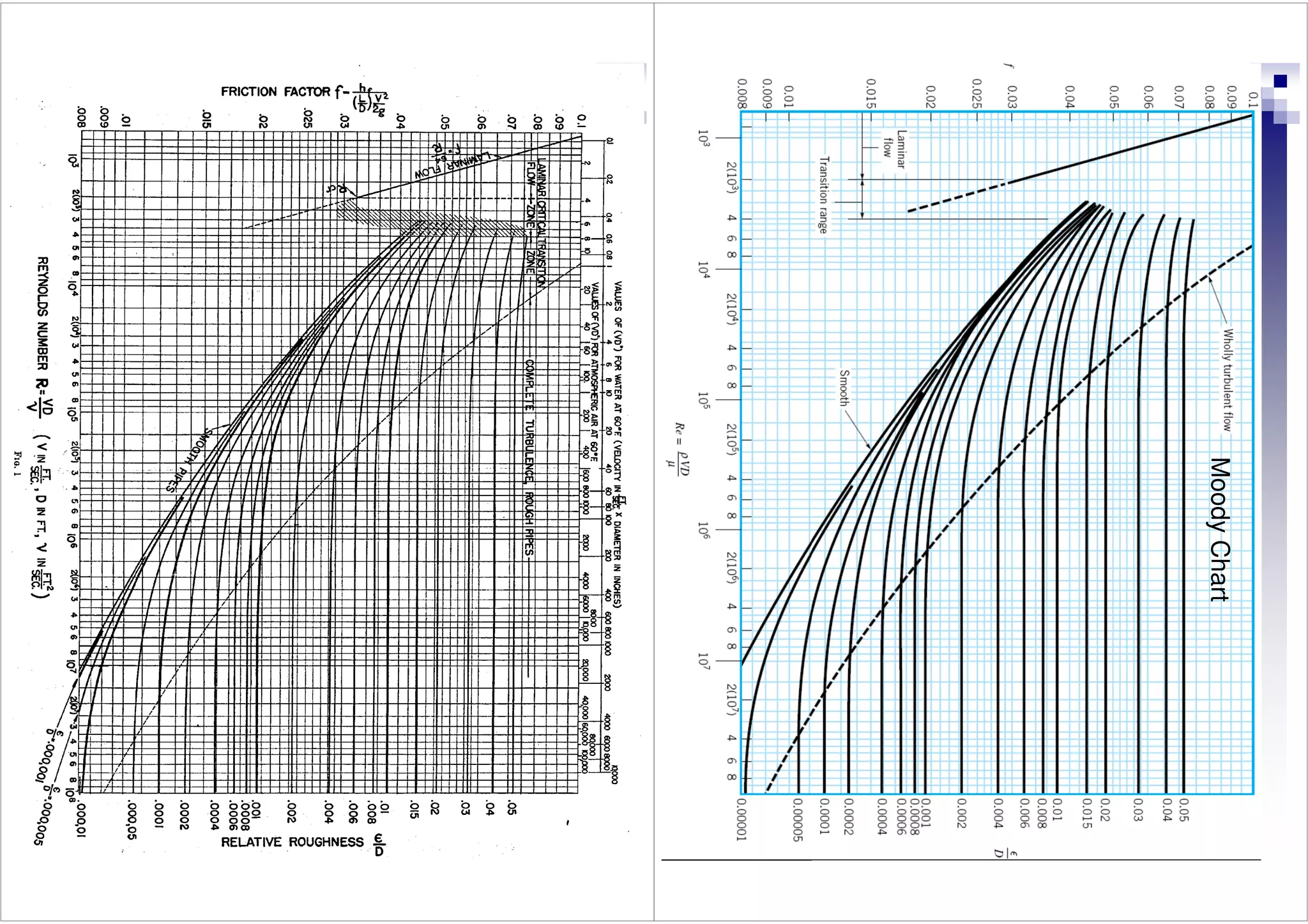
This document discusses flow in pipes. It covers different types of pipe flow including steady/unsteady and laminar/turbulent. The governing equations for pipe flow are presented, including continuity, momentum, and energy equations. Velocity profiles for laminar and turbulent flow are shown. Common pipe flow problems involve specifying a flowrate and calculating the required pressure difference to overcome friction losses.

1. Flow
in
Pipes
Chapter
8
Flow
in
Pipes
Pipe
flow
types
include
steady
or
unsteady,
uniform
or
non-
uniform,
and
laminar
or
turbulent
flow.
In
engineering
applications
such
as
in
oil
and
water
pipelines
flow
in
pipes
is
maintained
for
long
durations
and
does
not
change
with
time
(steady
flow).
Fluids
are
pumped
through
long
straight
pipes
such
that
the
velocity
vector
does
not
change
in
magnitude
or
direction
from
place
to
place
along
the
length
of
the
pipe
(uniform
flow).
Also,
it
is
expected
that
in
many
practical
applications
of
pipe
flow
and
because
of
economical
reasons,
the
flow
will
be
turbulent
flow
and
not
laminar
flow.
This
chapter
is
concerned
mostly
with
steady,
uniform,
turbulent
flow
of
real
fluids
in
pipes.
The
term
velocity
means
the
average
or
mean
velocity,
V
ave
.,
where
V
ave
=
Q/Area

2. 2.
Governing
Equations
The
descriptive
relations
in
pipe
flow
include
the
continuity
equation,
the
momentum
equation,
and
the
energy
equation.
Additional
useful
relation
is
that
of
the
Reynolds
number.
These
equations
are
as
follows:
Continuity
Equation
(Conservation
of
mass)
Compressible
flow
ρ
ρ
ρ
ρ
1
A
1
V
1
=
ρ
ρ
ρ
ρ
2
A
2
V
2
Incompressible
flow
Q
=
A
1
V
1
=
A
2
V
2
Where
ρ
ρ
ρ
ρ
1
,
ρ
ρ
ρ
ρ
2
=
density
at
the
pipe
entrance
and
exit
=
kg/m
3
ρ
ρ
ρ
ρ
1
=
ρ
ρ
ρ
ρ
2
for
incompressible
flow
A
1
,
A
2
=
pipe
entrance
and
exit
cross
section
area,
(m
2
)
ft
2
V
1
,
V
2
=
pipe
entrance
and
exit
average
flow
velocity,
ft/sec
(m/s)
=
mass
flow
rate,
kg/s,
Q
=
volume
flow
rate,
(m
3
/s)
ft
3
/sec,
2
1
m
m
=
m
Bernoulli’s
Equation
(Conservation
of
energy)
where
p
1
,
p
2
=
pipe
entrance
and
exit
static
pressures
z
1
,
z
2
=
entrance
and
exit
height
from
a
datum
(at
the
pump
centerline),
where
above
is
positive,
below
is
negative,
m
(ft)
h
L
=
energy
or
head
loss
due
to
friction,
entrance,
and
fittings,
(m)
g
=gravitational
Acceleration
=
9.81
m/s
2
=
32.2
ft/sec
2
The
velocity
head
or
kinetic
energy
term
V
2
/2g
is
based
on
an
average
or
uniform
velocity
over
the
pipe
cross
section.
Z
p
g
V
H
Energy
Total
+
+
=
γ
2
:
2
2
1
2
2
2
2
1
1
2
1
2
2
−
+
+
+
=
+
+
l
h
Z
p
g
V
Z
p
g
V
γ
γ
Incompressible
Flow:
Real
Flow

3. Velocity
Distributions
Velocity
Distributions
Laminar
flow
Turbulent
flow
)
1
(
(max)
)
(
2
2
1
1
o
r
r
v
r
v
−
=
7
/
1
1
1
)
1
(
(max)
)
(
o
r
r
v
r
v
−
=
Where
r
o
=
pipe
radius,
r
=
radial
distance
from
the
pipe
centerline
V
1
=
average
velocity
The
velocity
profiles
for
these
Equations
are
illustrated
on
the
next
slide.
Pipe
flow
Velocity
Profiles
7
/
1
1
1
)
1
(
(max)
)
(
o
r
r
v
r
v
−
=
)
1
(
(max)
)
(
2
2
1
1
o
r
r
v
r
v
−
=
Turbulent
Laminar

4. Velocity
Profiles
Laminar
OR
Turbulent
Flow
issuing
at
constant
speed
from
a
pipe:
(
a
)
high-viscosity,
low-Reynolds-number,
laminar
flow;
(
b
)
low-viscosity,
high-Reynolds-number,
turbulent
flow.

5. Reynolds
Experiment
Reynolds’
sketches
of
pipe-flow
transition:
(
a
)
low-speed,
laminar
flow;
(
b
)
high-speed,turbulent
flow;
(
c
)
spark
photograph
of
condition
(
b
).
VIDEO
Reynolds
Experiment
Reynolds
Experiment

6. Reynolds
Experiment
Dye
Reservoir
Liquid
flows
smoothly
through
the
bell-shape
inlet
and
dye
flows
through
the
center
line
Laminar
or
turbulent.
You
can
see
from
this
part
of
the
transparent
pipe.
Flow
rate
may
be
measured
by
filling
a
known
volume
while
measuring
the
time.
Flow
rate
(velocity,
Reynolds
number)
is
controlled
using
this
valve.
Over
flow
pipe
Energy
Losses:
Friction
Losses
Force
Viscous
Force
Inertia
Vd
Vd
R
e
=
=
=
ν
µ
ρ
g
V
d
l
f
h
lf
2
2
=
g
V
d
l
f
h
lf
2
2
=
Reynolds
Number
Laminar
Flow
:
For
Laminar
Flow
Re
2000
Friction
is
only
between
the
fluid
layers,
no
friction
between
the
fluid
and
the
pipe
walls.
e
R
f
64
=
and
Friction
Head
Loss,
h
lf
ρ
µ
ν
=
,

7. Transition
Turbulent
flow
When
fluid
flows
at
higher
flowrates,
the
flow
is
not
laminar.
Generally,
the
flow
field
will
vary
in
both
space
and
time
with
fluctuations
that
comprise
turbulence
For
this
case
there
is
no
simple
(exact)
solution
∆
∆
∆
∆
P
=
∆
∆
∆
∆
P
(D,
µ
µ
µ
µ
,
ρ
ρ
ρ
ρ
,
L,
V,ε
ε
ε
ε
)
u
z
ú
z
U
z
average
u
r
ú
r
U
r
average
p
P’
p
average
Time

8. Turbulent
flow
The
Friction
head
loss
expression
is
the
same
as
that
of
laminar
flow
but
the
friction
coefficient
is
different
because
the
friction
is
between
the
fluid
layers
and
between
the
fluid
and
the
pipe
walls:
g
V
d
l
f
h
lf
2
2
=
)
/
,
(
d
R
f
f
e
ε
=
with
Where:
ε
is
the
roughness,
mm
(in)
And
ε/d
is
the
relative
roughness,
dimensionless
Friction
Factor
for
Laminar
and
Turbulent
flows
Nikuradse
(1933)
Re

9. [
]
8
0
Re
log
0
2
1
.
*
*
.
−
=
f
f
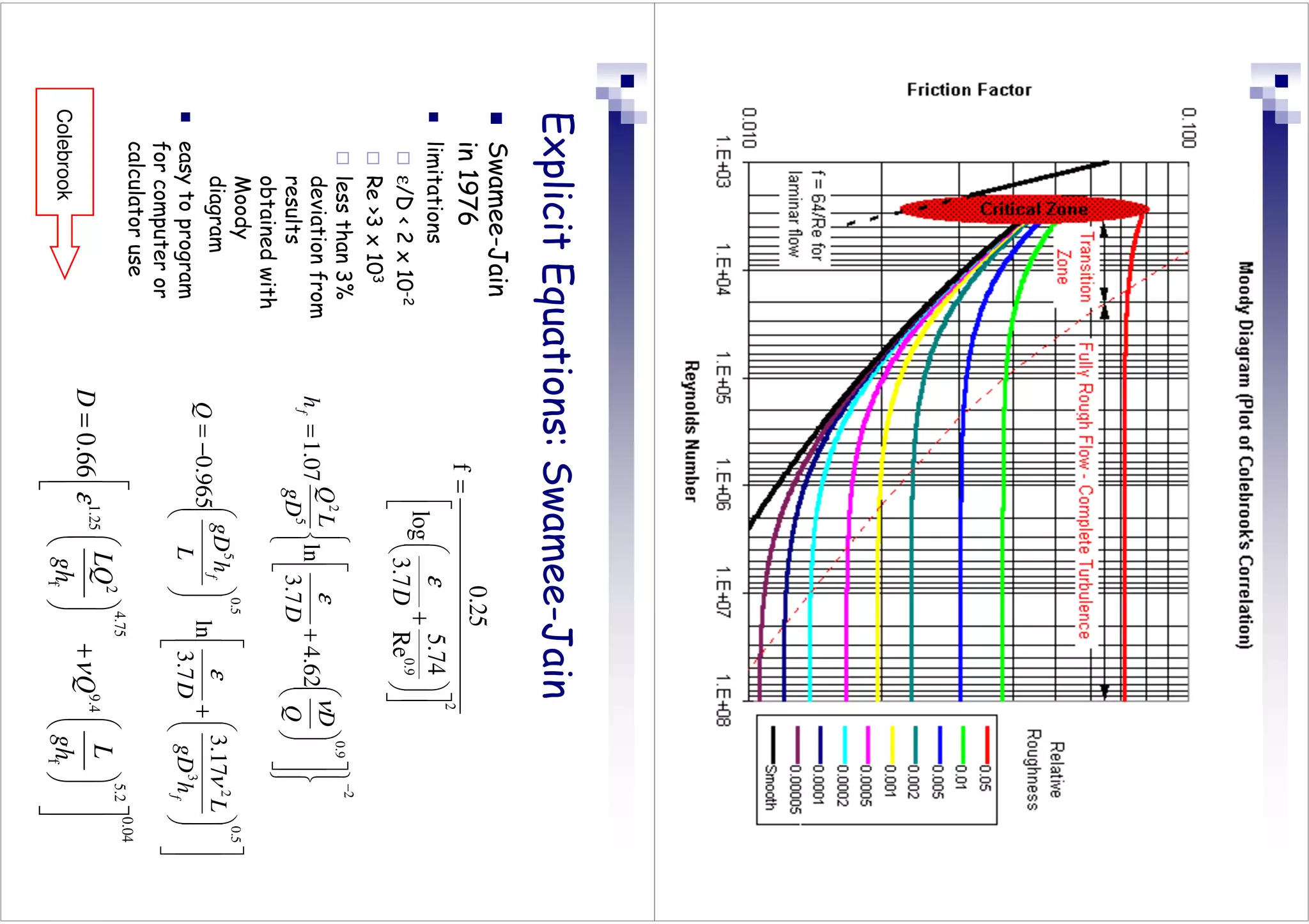
a-Smooth
pipe,
Re4000
f
≠
f
(ε/d)
14
.
1
log
0
2
1
+
−
=
D
f
ε
*
.
b-
Rough
pipe,
[
(D/ε)/(Re√ƒ)
0.01],
f
≠
f
(Re)
)
Re
51
.
2
7
.
3
/
log(
0
2
1
f
D
f
+
−
=
ε
*
.
c
-Transition
function
for
both
smooth
and
rough
pipe
(Colebrook)
25
.
0
Re
316
.
0
−
=
f
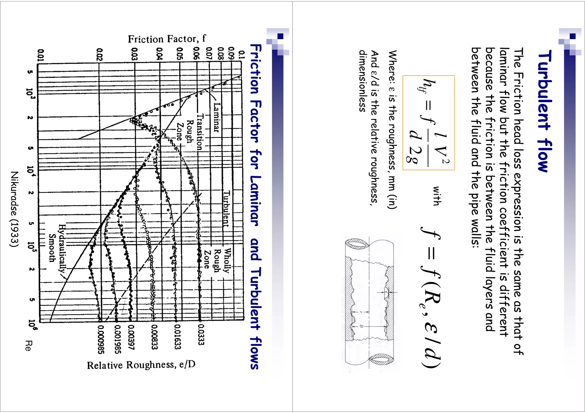
g
V
d
l
f
h
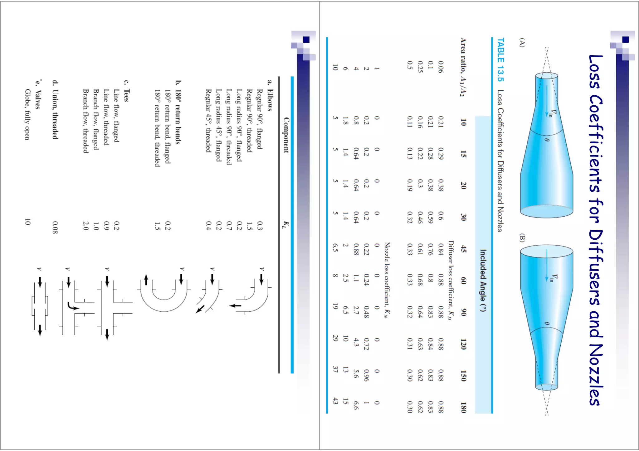
lf
2
2
=
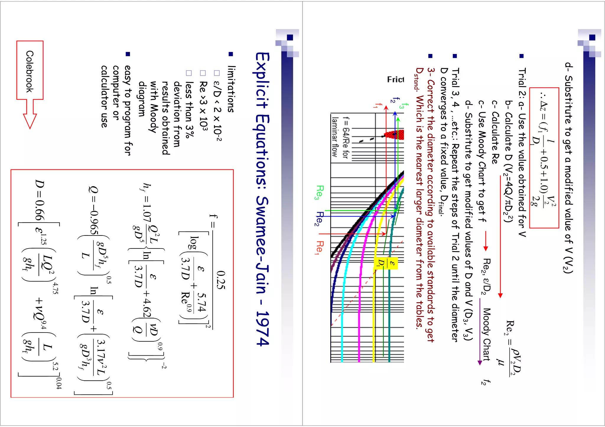
Empirical
Correlations
Friction
Factor
for
Turbulent
flow
Values
of
Equivalent
Roughness
(new
pipes)

10. Moody
Chart

11. Explicit
Equations:
Swamee-Jain
Swamee-Jain
in
1976
limitations
ε/D
2
x
10
-2
Re
3
x
10
3
less
than
3%
deviation
from
results
obtained
with
Moody
diagram
easy
to
program
for
computer
or
calculator
use
2
9
.
0
5
2
62
.
4
7
.
3
ln
07
.
1
−


























+
=
Q
D
D
gD
L
Q
h
f
ν
ε
0.04
4.75
5.2
2
1.25
9.4
f
f
0.66
LQ
L
D
Q
gh
gh
ε
ν






=
+














2
0.9
0.25
f
5.74
log
3.7
Re
D
ε
=




+
























+








−
=
5
.
0
3
2
5
.
0
5
17
.
3
7
.
3
ln
965
.
0
f
f
h
gD
L
D
L
h
gD
Q
ν
ε
Colebrook

12. Minor
(Secondary)
Losses
g
V
D
L
f
g
V
K
g
p
h
eq
b
b
2
2
2
2
=
=
∆
=
ρ
Bend
Characteristics
of
the
flow
in
a
90
bend
and
the
associated
loss
coefficient.

13. Character
of
the
flow
in
a
90°
°
°
°
mitered
bend
and
the
associated
loss
coefficient:
(a)
without
guide
vanes,
(b)
with
guide
vanes
Energy
Loss
in
Valves
(a)
gate
valve,
(b)
globe
valve,
(c)
angle
globe
(d)
swing
check
valve,
(d)
Gate
valve

14. Energy
Loss
in
Valves
Internal
structure
of
various
valves:
(
a
)
globe
valve,
(
b
)
gate
valve,
(
c
)
swing
check
valve,
(
d
)
stop
check
valve
Energy
Loss
in
Valves
Function
of
valve
type
and
valve
position
The
complex
flow
path
through
valves
can
result
in
high
head
loss
h
v
is
the
loss
in
terms
of
velocity
heads
g
V
D
L
f
g
V
K
p
h
eq
v
v
2
2
2
2
=
=
∆
=
γ
L
eq
=
equivalent
length
=
Additional
length
of
the
pipe
to
cause
same
losses
as
the
valve.
Butterfly
valve

15. Friction
Loss
Factors
for
valves
Valve
K
L
eq
/D
Gate
valve,
wide
open
0.15
7
Gate
valve,
3/4
open
0.85
40
Gate
valve,
1/2
open
4.4
200
Gate
valve,
1/4
open
20
900
Globe
valve,
wide
open
7.5
350
g
V
D
L
f
g
V
K
p
h
eq
v
v
2
2
2
2
=
=
∆
=
γ
Entrance
Losses
(
c
)
slightly
rounded,
K
L
=
0.2,
(
d
)
well-rounded,
K
L
=
0.04
(
a
)
Reentrant,
K
L
=
0.8,
(
b
)
sharp-edged,
K
L
=
0.5
(default)

16. Loss
coefficient
for
a
sudden
contraction
0.5?
Exit
Losses
(a)
Reentrant,
K
L
=
1.0,
(b)
Sharp-edged,
K
L
=
1.0
(c)
Slightly
rounded,
K
L
=
1.0
(b)
Well-rounded,
K
L
=
1.0
Tank

17. Loss
coefficient
for
a
sudden
expansion
Loss
coefficient
for
a
typical
conical
diffuser

18. Loss
Coefficients
for
Diffusers
and
Nozzles

19. Pipe
Flow
Problems
In
a
Type
I
problem
we
specify
the
desired
flowrate
or
average
velocity
and
determine
the
necessary
pressure
difference
or
head
loss.
For
example,
if
a
flowrate
of
2.0
gpm
is
required
for
a
dishwasher
that
is
connected
to
the
water
heater
by
a
given
pipe
system,
what
pressure
is
needed
in
the
water
heater?
In
a
Type
II
problem
we
specify
the
applied
driving
pressure
or,
alternatively,
the
head
loss
and
determine
the
flowrate.
For
example,
how
many
gpm
of
hot
water
are
supplied
to
the
dishwasher
if
the
pressure
within
the
water
heater
is
60
psi
and
the
pipe
system
details
(length,
diameter,
roughness
of
the
pipe;
number
of
elbows;
etc.)
are
specified?
In
a
Type
III
problem
we
specify
the
pressure
drop
and
the
flowrate
and
determine
the
diameter
of
the
pipe
needed.
For
example,
what
diameter
of
pipe
is
needed
between
the
water
heater
and
dishwasher
if
the
pressure
in
the
water
heater
is
60
psi
(determined
by
the
city
water
system)
and
the
flowrate
is
to
be
not
less
than
2.0
gpm
(determined
by
the
manufacturer)?

20. Pipe
Flow
Problems
Types
Type
I
Problems
Given:
ρ
and
µ
of
the
fluid
Material
(ε),
D
and
L
of
the
pipe
Flow
rate,
Q
Required:
ΔZ
OR
ΔP
Solution:
1-
Apply
Bernoulli
eqn
z
z
z
∆
=
−
2
1
g
V
K
g
V
D
l
f
z
g
V
p
z
g
V
p
L
2
2
2
2
2
2
2
2
2
2
1
2
1
1
∑
+
+
+
+
=
+
+
γ
γ
0
2
2
,
0
2
2
2
1
2
1
=
=
=
=
g
V
g
V
p
p
γ
γ
g
V
K
D
l
f
z
L
2
)
(
2
∑
+
=
∆
2-
Determine
f
µ
ρ
π
VD
and
D
Q
Area
Q
V
=
=
=
Re
4
/
2
Re,
ε/D
Moody
Chart
f
g
V
D
l
f
z
2
)
0
.
1
5
.
0
(
2
+
+
=
∆
∴
3-
Substitute
note
0
2
2
,
0
2
2
2
1
2
1
=
=
=
=
g
V
g
V
p
p
γ
γ
1
2

21. Type
II
Problems
Given:
ρ
and
µ
of
the
fluid
Material
(ε),
D
and
L
of
the
pipe
Energy
difference,
ΔZ
OR
ΔP
Required:
Flow
rate
Q
Solution:
1-
Apply
Bernoulli
eqn
0
2
2
,
0
2
2
2
1
2
1
=
=
=
=
g
V
g
V
p
p
γ
γ
z
z
z
∆
=
−
2
1
g
V
K
g
V
D
l
f
z
g
V
p
z
g
V
p
L
2
2
2
2
2
2
2
2
2
2
1
2
1
1
∑
+
+
+
+
=
+
+
γ
γ
0
2
2
,
0
2
2
2
1
2
1
=
=
=
=
g
V
g
V
p
p
γ
γ
g
V
K
D
l
f
z
L
2
)
(
2
∑
+
=
∆
2-
Determine
f
(Trial
and
Error)
Trial
1:
a-
Assume
an
initial
value
of
V
(1-3
m/s)
b-
calculate
Re
c-
Use
Moody
Chart
to
get
f
µ
ρ
D
V
1
1
Re
=
Re
1
,
ε/D
Moody
Chart
f
1
note
0
2
2
,
0
2
2
2
1
2
1
=
=
=
=
g
V
g
V
p
p
γ
γ
1
2
Optimum
Diameter
of
a
Pipe
(Economical
Velocity)
Economics
drives
designs.
To
optimize
piping
diameter,
engineers
frequently
use
rules-of-
thumb
that
speed
up
calculations.
But
the
data
underlying
such
rules
must
always
be
verified.
Changes
in
design
variables
cause
some
costs
to
increase
while
others
decrease.
Total
cost
is
the
sum
of
fixed
costs
and
variable
costs.
There
is
always
a
set
of
values
at
which
the
total
costs
are
a
minimum.
At
the
optimum
diameter,
the
economical
velocity
is
from
1
to
3
m/s

22. d-
Substitute
to
get
a
modified
value
of
V
(V
2
)
µ
ρ
D
V
2
2
Re
=
Re
2
,
ε/D
Moody
Chart
f
2
g
V
D
l
f
z
2
)
0
.
1
5
.
0
(
2
2
1
+
+
=
∆
∴
Trial
2:
a-
Use
the
value
obtained
for
V
b-
Calculate
Re
c-
Use
Moody
Chart
to
get
f
d-
Substitute
to
get
a
modified
value
of
V
(V
3
)
Trial
3,
4
,
…etc.:
Repeat
the
steps
of
Trial
2
until
the
velocity
V
converges
to
a
fixed
value,
V
final
.
3-
Substitute
to
get
the
flow
rate:
Q=
V
final
*
Area
D
ε
Re
1
f
1
f
2
Re
2
Re
3
f
3
Type
III
Problems
Given:
ρ
and
µ
of
the
fluid
Material
(ε)
and
L
of
the
pipe
Flow
rate,
Q
and
ΔZ
OR
ΔP
Required:
D
Solution:
1-
Apply
Bernoulli
eqn
0
2
2
,
0
2
2
2
1
2
1
=
=
=
=
g
V
g
V
p
p
γ
γ
z
z
z
∆
=
−
2
1
g
V
K
g
V
D
l
f
z
g
V
p
z
g
V
p
L
2
2
2
2
2
2
2
2
2
2
1
2
1
1
∑
+
+
+
+
=
+
+
γ
γ
0
2
2
,
0
2
2
2
1
2
1
=
=
=
=
g
V
g
V
p
p
γ
γ
g
V
K
D
l
f
z
L
2
)
(
2
∑
+
=
∆
2-
Determine
f
(Trial
and
Error)
Trial
1:
a-
Assume
an
initial
value
of
V
(1-3
m/s)
b-
Calculate
an
initial
value
of
D
(V
1
=4Q/πD
1
2
)
c-
calculate
Re
d-
Use
Moody
Chart
to
get
f
µ
ρ
1
1
1
Re
D
V
=
Re
1
,
ε/D
1
Moody
Chart
f
1
note
0
2
2
,
0
2
2
2
1
2
1
=
=
=
=
g
V
g
V
p
p
γ
γ
1
2

23. µ
ρ
2
2
2
Re
D
V
=
Re
2
,
ε/D
2
Moody
Chart
f
2
d-
Substitute
to
get
a
modified
value
of
V
(V
2
)
g
V
D
l
f
z
2
)
0
.
1
5
.
0
(
2
2
1
1
+
+
=
∆
∴
Trial
2:
a-
Use
the
value
obtained
for
V
b-
Calculate
D
(V
2
=4Q/πD
2
2
)
c-
Calculate
Re
c-
Use
Moody
Chart
to
get
f
d-
Substitute
to
get
modified
values
of
D
and
V
(D
3
,
V
3
)
Trial
3,
4
,
…etc.:
Repeat
the
steps
of
Trial
2
until
the
diameter
D
converges
to
a
fixed
value,
D
final
.
3-
Correct
the
diameter
according
to
available
standards
to
get
D
stand
.
Which
is
the
nearest
larger
diameter
from
the
tables.
1
D
ε
Re
1
f
1
f
2
Re
2
Re
3
f
3
Explicit
Equations:
Swamee-Jain
-
1974
limitations
ε/D
2
x
10
-2
Re
3
x
10
3
less
than
3%
deviation
from
results
obtained
with
Moody
diagram
easy
to
program
for
computer
or
calculator
use
2
9
.
0
5
2
62
.
4
7
.
3
ln
07
.
1
−


























+
=
Q
D
D
gD
L
Q
h
f
ν
ε
0.04
4.75
5.2
2
1.25
9.4
f
f
0.66
LQ
L
D
Q
gh
gh
ε
ν






=
+














2
0.9
0.25
f
5.74
log
3.7
Re
D
ε
=




+
























+








−
=
5
.
0
3
2
5
.
0
5
17
.
3
7
.
3
ln
965
.
0
f
f
h
gD
L
D
L
h
gD
Q
ν
ε
Colebrook

24. Multiple
Pipe
Systems
Pipes
in
Series
One
of
the
simplest
multiple
pipe
systems
is
that
containing
pipes
in
series
.
Every
fluid
particle
that
passes
through
the
system
passes
through
each
of
the
pipes.
Thus,
the
flowrate
(but
not
the
velocity)
is
the
same
in
each
pipe,
and
the
head
loss
from
point
A
to
point
B
is
the
sum
of
the
head
losses
in
each
of
the
pipes.








=
=
i
i
i
i
i
D
D
V
f
f
ε
µ
ρ
,
Re
In
general,
the
friction
factors
will
be
different
for
each
pipe
because
the
Reynolds
numbers
and
the
relative
roughnesses
will
be
different.
3
2
1
3
2
1
L
L
L
L
h
h
h
h
and
Q
Q
Q
B
A
+
+
=
=
=
−
Pipes
in
Parallel
In
this
system
a
fluid
particle
traveling
from
A
to
B
may
take
any
of
the
paths
available,
with
the
total
flowrate
equal
to
the
sum
of
the
flowrates
in
each
pipe.
However,
by
writing
the
energy
equation
between
points
A
and
B
it
is
found
that
the
head
loss
experienced
by
any
fluid
particle
traveling
between
these
locations
is
the
same,
independent
of
the
path
taken.
3
2
1
3
2
1
L
L
L
L
B
A
h
h
h
h
and
Q
Q
Q
Q
B
A
=
=
=
+
+
=
−
−

25. Multiple
Pipe
Loop
System
3
1
2
1
3
2
1
L
L
L
L
L
L
B
A
h
h
h
h
h
h
Q
Q
Q
Q
B
A
B
A
+
=
+
=
+
=
=
−
−
−
Three
equations
in
three
unknowns:
Q
1
,
Q
2
,
Q
3
OR
V
1
,
V
2
,
V
3
3
2
L
L
h
h
=
Note
that
Three-Tank
Problem
3
2
3
1
2
1
3
L
L
L
L
L
L
C
A
B
A
h
h
h
h
h
h
Q
Q
Q
Q
Q
C
B
C
A
+
=
+
=
+
=
=
+
−
−
−
−
Condition1:
If
the
flow
is
from
A
to
B
and
C
Condition
2:
If
the
flow
is
from
A
and
B
to
C
3
1
2
1
3
2
1
L
L
L
L
L
L
C
A
B
A
h
h
h
h
h
h
Q
Q
Q
Q
Q
C
A
B
A
+
=
+
=
+
=
=
+
−
−
−
−
OR

26. Pumps
and
Turbines
The
mechanical
energy
loss
due
to
frictional
effects
causes
the
TEL
and
HGL
to
slope
downward
in
the
direction
of
flow.
A
steep
jump
occurs
in
TEL
and
HGL
whenever
mechanical
energy
is
added
to
the
fluid
by
a
pump.
Likewise,
a
steep
drop
occurs
in
EGL
and
HGL
whenever
mechanical
energy
is
removed
from
the
fluid
by
a
turbine.
Bernoulli’s
equation
may
be
written
as:
E
in
=
E
out
+
E
loss
.
g
V
K
g
V
D
l
f
H
z
g
V
p
H
z
g
V
p
L
Turbine
pump
2
2
2
2
2
2
2
2
2
2
1
2
1
1
∑
+
+
+
+
+
=
+
+
+
γ
γ