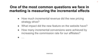
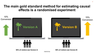
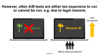
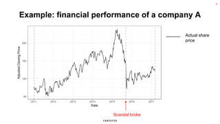
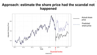
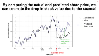
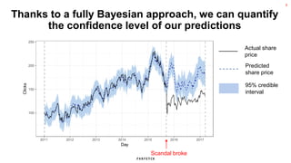
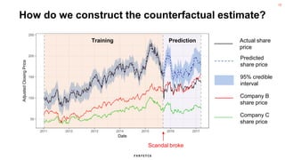
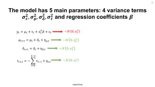
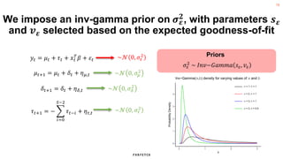
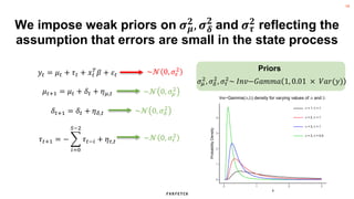
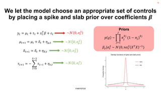
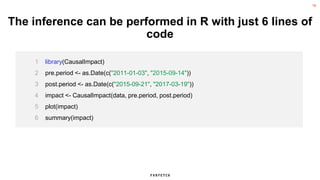
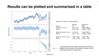
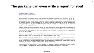
1
Causal Inference in R
Ana Daglis, Farfetch
2
Farfetch
Customer
Customer
Customer
Customer
Customer
Boutique
Boutique
Boutique
Boutique
Boutique
3
One of the most common questions we face in
marketing is measuring the incremental effects
● How much incremental revenue did the new pricing
strategy drive?
● What impact did the new feature on the website have?
● How many incremental conversions were achieved by
increasing the commission rate for our affiliates?
● …
4
The main gold standard method for estimating causal
effects is a randomised experiment
10%
Conversion
15%
Conversion
50% of visitors see Version B
Version B
Version A
50% of visitors see Version A
5
However, often A/B tests are either too expensive to run
or cannot be run, e.g. due to legal reasons
15%
Conversion
100% of visitors see Version B
Version B
Version A
6
Example: financial performance of a company A
80
120
160
200
2011 2012 2013 2014 2015 2016 2017
Date
Adjusted
Closing
Price
Scandal broke
Actual share
price
7
Approach: estimate the share price had the scandal not
happened
100
150
200
2011 2012 2013 2014 2015 2016 2017
Date
Adjusted
Closing
Price
Scandal broke
Actual share
price
Predicted
share price
8
By comparing the actual and predicted share price, we
can estimate the drop in stock value due to the scandal
100
150
200
2011 2012 2013 2014 2015 2016 2017
Date
Adjusted
Closing
Price
Scandal broke
Drop in stock
value due to
scandal
Actual share
price
Predicted
share price
9
Thanks to a fully Bayesian approach, we can quantify
the confidence level of our predictions
100
150
200
250
2011 2012 2013 2014 2015 2016 2017
Day
Clicks
Scandal broke
Actual share
price
Predicted
share price
95% credible
interval
10
How do we construct the counterfactual estimate?
50
100
150
200
250
2011 2012 2013 2014 2015 2016 2017
Date
Adjusted
Closing
Price
Actual share
price
Predicted
share price
95% credible
interval
Company B
share price
Company C
share price
Training Prediction
Scandal broke
11
Causal Impact methodology is based on a Bayesian
structural time series model
𝑦𝑡 = 𝑍𝑡
𝑇
𝛼𝑡 + 𝜀𝑡
𝛼𝑡+1 = 𝑇𝑡
𝑇
𝛼𝑡 + 𝑅𝑡𝜂𝑡
Causal Impact model
Most general form of the model
Observation equation
State equation
𝑦𝑡 = 𝜇𝑡 + 𝜏𝑡 + 𝑥𝑡
𝑇
𝛽 + 𝜀𝑡
𝜇𝑡+1 = 𝜇𝑡 + 𝛿𝑡 + 𝜂𝜇,𝑡
𝛿𝑡+1 = 𝛿𝑡 + 𝜂𝛿,𝑡
𝜏𝑡+1 = −
𝑖=0
𝑆−2
𝜏𝑡−𝑖 + 𝜂𝜏,𝑡
12
The model has 5 main parameters: 4 variance terms
𝝈𝜺
𝟐
, 𝝈𝝁
𝟐
, 𝝈𝜹
𝟐
, 𝝈𝝉
𝟐
and regression coefficients 𝜷
𝑦𝑡 = 𝜇𝑡 + 𝜏𝑡 + 𝑥𝑡
𝑇
𝛽 + 𝜀𝑡
𝜇𝑡+1 = 𝜇𝑡 + 𝛿𝑡 + 𝜂𝜇,𝑡
𝛿𝑡+1 = 𝛿𝑡 + 𝜂𝛿,𝑡
𝜏𝑡+1 = −
𝑖=0
𝑆−2
𝜏𝑡−𝑖 + 𝜂𝜏,𝑡
~𝒩 0, 𝜎𝜀
2
~𝒩 0, 𝜎𝜇
2
~𝒩 0, 𝜎𝛿
2
~𝒩 0, 𝜎𝜏
2
13
We impose an inv-gamma prior on 𝝈𝜺
𝟐
, with parameters 𝒔𝜺
and 𝒗𝜺 selected based on the expected goodness-of-fit
𝑦𝑡 = 𝜇𝑡 + 𝜏𝑡 + 𝑥𝑡
𝑇
𝛽 + 𝜀𝑡
𝜇𝑡+1 = 𝜇𝑡 + 𝛿𝑡 + 𝜂𝜇,𝑡
𝛿𝑡+1 = 𝛿𝑡 + 𝜂𝛿,𝑡
𝜏𝑡+1 = −
𝑖=0
𝑆−2
𝜏𝑡−𝑖 + 𝜂𝜏,𝑡
~𝒩 0, 𝜎𝜀
2
~𝒩 0, 𝜎𝜇
2
~𝒩 0, 𝜎𝛿
2
~𝒩 0, 𝜎𝜏
2
Priors
𝜎𝜀
2
~ 𝐼𝑛𝑣−𝐺𝑎𝑚𝑚𝑎 𝑠𝜀, 𝑣𝜀
0
1
2
3
4
0 1 2 3
x
Probability
Density
a = 1, b = 1
a = 2, b = 1
a = 3, b = 1
a = 3, b = 0.5
Inv−Gamma(a,b) density for varying values of a and b
14
We impose weak priors on 𝝈𝝁
𝟐, 𝝈𝜹
𝟐
and 𝝈𝝉
𝟐 reflecting the
assumption that errors are small in the state process
𝑦𝑡 = 𝜇𝑡 + 𝜏𝑡 + 𝑥𝑡
𝑇
𝛽 + 𝜀𝑡
𝜇𝑡+1 = 𝜇𝑡 + 𝛿𝑡 + 𝜂𝜇,𝑡
𝛿𝑡+1 = 𝛿𝑡 + 𝜂𝛿,𝑡
𝜏𝑡+1 = −
𝑖=0
𝑆−2
𝜏𝑡−𝑖 + 𝜂𝜏,𝑡
~𝒩 0, 𝜎𝜀
2
~𝒩 0, 𝜎𝜇
2
~𝒩 0, 𝜎𝛿
2
~𝒩 0, 𝜎𝜏
2
Priors
𝜎𝜇
2
, 𝜎𝛿
2
, 𝜎𝜏
2
~ 𝐼𝑛𝑣−𝐺𝑎𝑚𝑚𝑎 1, 0.01 × 𝑉𝑎𝑟(𝑦)
0
1
2
3
4
0 1 2 3
x
Probability
Density
a = 1, b = 1
a = 2, b = 1
a = 3, b = 1
a = 3, b = 0.5
Inv−Gamma(a,b) density for varying values of a and b
15
We let the model choose an appropriate set of controls
by placing a spike and slab prior over coefficients 𝜷
𝑦𝑡 = 𝜇𝑡 + 𝜏𝑡 + 𝑥𝑡
𝑇
𝛽 + 𝜀𝑡
𝜇𝑡+1 = 𝜇𝑡 + 𝛿𝑡 + 𝜂𝜇,𝑡
𝛿𝑡+1 = 𝛿𝑡 + 𝜂𝛿,𝑡
𝜏𝑡+1 = −
𝑖=0
𝑆−2
𝜏𝑡−𝑖 + 𝜂𝜏,𝑡
~𝒩 0, 𝜎𝜀
2
~𝒩 0, 𝜎𝜇
2
~𝒩 0, 𝜎𝛿
2
~𝒩 0, 𝜎𝜏
2
Priors
𝛽𝛾|𝜎𝜀
2
~ 𝒩(0, 𝑛𝜎𝜀
2
𝑋𝑇
𝑋 −1
)
𝑝 𝜚 ~
𝑗=1
𝐽
𝜋𝑗
𝜚𝑗
(1 − 𝜋𝑗)
𝜚𝑗
0
1
2
3
4
−2 −1 0 1 2
x
Probability
Density
Spike
Slab
Density functions of spike and slab priors
16
The inference can be performed in R with just 6 lines of
code
1 library(CausalImpact)
2 pre.period <- as.Date(c("2011-01-03", "2015-09-14"))
3 post.period <- as.Date(c("2015-09-21", "2017-03-19"))
4 impact <- CausalImpact(data, pre.period, post.period)
5 plot(impact)
6 summary(impact)
17
Results can be plotted and summarised in a table
original
pointwise
cumulative
2011 2012 2013 2014 2015 2016 2017
100
150
200
250
−80
−40
0
−4000
−3000
−2000
−1000
0
Date
Adjusted
Closing
Price
Cumulative panel only makes sense when the metric is
additive, such as clicks or the number of orders, but not
in the case when it is a share price
18
The package can even write a report for you!
19
Additional considerations
● It is important that covariates included in the model are not
themselves affected by the event. For each covariate included,
it is critical to reason why this is the case.
● The model can be validated by running the Causal Impact
analysis on an ‘imaginary event’ before the actual event. We
should not be seeing any significant effect, and actual and
predicted lines should match reasonably closely before the actual
event.
20
References
● K.H. Brodersen, F. Gallusser, J. Koehler, N. Remy, S. L. Scott,
(2015). Inferring Causal Impact Using Bayesian Structural Time-
Series Models.
https://research.google.com/pubs/pub41854.html.
● S. L. Scott, H. Varian, (2013). Predicting the Present with
Bayesian Structural Time Series.
https://people.ischool.berkeley.edu/~hal/Papers/2013/pred-
present-with-bsts.pdf.
21
Thank you!

Causal Inference in R

  • 1.
    1 Causal Inference inR Ana Daglis, Farfetch
  • 2.
  • 3.
    3 One of themost common questions we face in marketing is measuring the incremental effects ● How much incremental revenue did the new pricing strategy drive? ● What impact did the new feature on the website have? ● How many incremental conversions were achieved by increasing the commission rate for our affiliates? ● …
  • 4.
    4 The main goldstandard method for estimating causal effects is a randomised experiment 10% Conversion 15% Conversion 50% of visitors see Version B Version B Version A 50% of visitors see Version A
  • 5.
    5 However, often A/Btests are either too expensive to run or cannot be run, e.g. due to legal reasons 15% Conversion 100% of visitors see Version B Version B Version A
  • 6.
    6 Example: financial performanceof a company A 80 120 160 200 2011 2012 2013 2014 2015 2016 2017 Date Adjusted Closing Price Scandal broke Actual share price
  • 7.
    7 Approach: estimate theshare price had the scandal not happened 100 150 200 2011 2012 2013 2014 2015 2016 2017 Date Adjusted Closing Price Scandal broke Actual share price Predicted share price
  • 8.
    8 By comparing theactual and predicted share price, we can estimate the drop in stock value due to the scandal 100 150 200 2011 2012 2013 2014 2015 2016 2017 Date Adjusted Closing Price Scandal broke Drop in stock value due to scandal Actual share price Predicted share price
  • 9.
    9 Thanks to afully Bayesian approach, we can quantify the confidence level of our predictions 100 150 200 250 2011 2012 2013 2014 2015 2016 2017 Day Clicks Scandal broke Actual share price Predicted share price 95% credible interval
  • 10.
    10 How do weconstruct the counterfactual estimate? 50 100 150 200 250 2011 2012 2013 2014 2015 2016 2017 Date Adjusted Closing Price Actual share price Predicted share price 95% credible interval Company B share price Company C share price Training Prediction Scandal broke
  • 11.
    11 Causal Impact methodologyis based on a Bayesian structural time series model 𝑦𝑡 = 𝑍𝑡 𝑇 𝛼𝑡 + 𝜀𝑡 𝛼𝑡+1 = 𝑇𝑡 𝑇 𝛼𝑡 + 𝑅𝑡𝜂𝑡 Causal Impact model Most general form of the model Observation equation State equation 𝑦𝑡 = 𝜇𝑡 + 𝜏𝑡 + 𝑥𝑡 𝑇 𝛽 + 𝜀𝑡 𝜇𝑡+1 = 𝜇𝑡 + 𝛿𝑡 + 𝜂𝜇,𝑡 𝛿𝑡+1 = 𝛿𝑡 + 𝜂𝛿,𝑡 𝜏𝑡+1 = − 𝑖=0 𝑆−2 𝜏𝑡−𝑖 + 𝜂𝜏,𝑡
  • 12.
    12 The model has5 main parameters: 4 variance terms 𝝈𝜺 𝟐 , 𝝈𝝁 𝟐 , 𝝈𝜹 𝟐 , 𝝈𝝉 𝟐 and regression coefficients 𝜷 𝑦𝑡 = 𝜇𝑡 + 𝜏𝑡 + 𝑥𝑡 𝑇 𝛽 + 𝜀𝑡 𝜇𝑡+1 = 𝜇𝑡 + 𝛿𝑡 + 𝜂𝜇,𝑡 𝛿𝑡+1 = 𝛿𝑡 + 𝜂𝛿,𝑡 𝜏𝑡+1 = − 𝑖=0 𝑆−2 𝜏𝑡−𝑖 + 𝜂𝜏,𝑡 ~𝒩 0, 𝜎𝜀 2 ~𝒩 0, 𝜎𝜇 2 ~𝒩 0, 𝜎𝛿 2 ~𝒩 0, 𝜎𝜏 2
  • 13.
    13 We impose aninv-gamma prior on 𝝈𝜺 𝟐 , with parameters 𝒔𝜺 and 𝒗𝜺 selected based on the expected goodness-of-fit 𝑦𝑡 = 𝜇𝑡 + 𝜏𝑡 + 𝑥𝑡 𝑇 𝛽 + 𝜀𝑡 𝜇𝑡+1 = 𝜇𝑡 + 𝛿𝑡 + 𝜂𝜇,𝑡 𝛿𝑡+1 = 𝛿𝑡 + 𝜂𝛿,𝑡 𝜏𝑡+1 = − 𝑖=0 𝑆−2 𝜏𝑡−𝑖 + 𝜂𝜏,𝑡 ~𝒩 0, 𝜎𝜀 2 ~𝒩 0, 𝜎𝜇 2 ~𝒩 0, 𝜎𝛿 2 ~𝒩 0, 𝜎𝜏 2 Priors 𝜎𝜀 2 ~ 𝐼𝑛𝑣−𝐺𝑎𝑚𝑚𝑎 𝑠𝜀, 𝑣𝜀 0 1 2 3 4 0 1 2 3 x Probability Density a = 1, b = 1 a = 2, b = 1 a = 3, b = 1 a = 3, b = 0.5 Inv−Gamma(a,b) density for varying values of a and b
  • 14.
    14 We impose weakpriors on 𝝈𝝁 𝟐, 𝝈𝜹 𝟐 and 𝝈𝝉 𝟐 reflecting the assumption that errors are small in the state process 𝑦𝑡 = 𝜇𝑡 + 𝜏𝑡 + 𝑥𝑡 𝑇 𝛽 + 𝜀𝑡 𝜇𝑡+1 = 𝜇𝑡 + 𝛿𝑡 + 𝜂𝜇,𝑡 𝛿𝑡+1 = 𝛿𝑡 + 𝜂𝛿,𝑡 𝜏𝑡+1 = − 𝑖=0 𝑆−2 𝜏𝑡−𝑖 + 𝜂𝜏,𝑡 ~𝒩 0, 𝜎𝜀 2 ~𝒩 0, 𝜎𝜇 2 ~𝒩 0, 𝜎𝛿 2 ~𝒩 0, 𝜎𝜏 2 Priors 𝜎𝜇 2 , 𝜎𝛿 2 , 𝜎𝜏 2 ~ 𝐼𝑛𝑣−𝐺𝑎𝑚𝑚𝑎 1, 0.01 × 𝑉𝑎𝑟(𝑦) 0 1 2 3 4 0 1 2 3 x Probability Density a = 1, b = 1 a = 2, b = 1 a = 3, b = 1 a = 3, b = 0.5 Inv−Gamma(a,b) density for varying values of a and b
  • 15.
    15 We let themodel choose an appropriate set of controls by placing a spike and slab prior over coefficients 𝜷 𝑦𝑡 = 𝜇𝑡 + 𝜏𝑡 + 𝑥𝑡 𝑇 𝛽 + 𝜀𝑡 𝜇𝑡+1 = 𝜇𝑡 + 𝛿𝑡 + 𝜂𝜇,𝑡 𝛿𝑡+1 = 𝛿𝑡 + 𝜂𝛿,𝑡 𝜏𝑡+1 = − 𝑖=0 𝑆−2 𝜏𝑡−𝑖 + 𝜂𝜏,𝑡 ~𝒩 0, 𝜎𝜀 2 ~𝒩 0, 𝜎𝜇 2 ~𝒩 0, 𝜎𝛿 2 ~𝒩 0, 𝜎𝜏 2 Priors 𝛽𝛾|𝜎𝜀 2 ~ 𝒩(0, 𝑛𝜎𝜀 2 𝑋𝑇 𝑋 −1 ) 𝑝 𝜚 ~ 𝑗=1 𝐽 𝜋𝑗 𝜚𝑗 (1 − 𝜋𝑗) 𝜚𝑗 0 1 2 3 4 −2 −1 0 1 2 x Probability Density Spike Slab Density functions of spike and slab priors
  • 16.
    16 The inference canbe performed in R with just 6 lines of code 1 library(CausalImpact) 2 pre.period <- as.Date(c("2011-01-03", "2015-09-14")) 3 post.period <- as.Date(c("2015-09-21", "2017-03-19")) 4 impact <- CausalImpact(data, pre.period, post.period) 5 plot(impact) 6 summary(impact)
  • 17.
    17 Results can beplotted and summarised in a table original pointwise cumulative 2011 2012 2013 2014 2015 2016 2017 100 150 200 250 −80 −40 0 −4000 −3000 −2000 −1000 0 Date Adjusted Closing Price Cumulative panel only makes sense when the metric is additive, such as clicks or the number of orders, but not in the case when it is a share price
  • 18.
    18 The package caneven write a report for you!
  • 19.
    19 Additional considerations ● Itis important that covariates included in the model are not themselves affected by the event. For each covariate included, it is critical to reason why this is the case. ● The model can be validated by running the Causal Impact analysis on an ‘imaginary event’ before the actual event. We should not be seeing any significant effect, and actual and predicted lines should match reasonably closely before the actual event.
  • 20.
    20 References ● K.H. Brodersen,F. Gallusser, J. Koehler, N. Remy, S. L. Scott, (2015). Inferring Causal Impact Using Bayesian Structural Time- Series Models. https://research.google.com/pubs/pub41854.html. ● S. L. Scott, H. Varian, (2013). Predicting the Present with Bayesian Structural Time Series. https://people.ischool.berkeley.edu/~hal/Papers/2013/pred- present-with-bsts.pdf.
  • 21.