This document describes a study that used Monte Carlo simulation to forecast user bandwidth utilization in a campus network. The study collected traffic data from a test campus network setup over 30 days. It analyzed the data to determine bandwidth usage patterns and categorized usage. It then used the data to develop a Monte Carlo simulation model that generated random numbers based on the actual usage data probability distribution. This allowed the model to forecast bandwidth utilization for different days, helping network planners understand demands and design network upgrades accordingly. The model and results help campus networks better plan for high and normal traffic loads to deliver content.

1. International Journal of Electrical and Computer Engineering (IJECE)
Vol. 10, No. 5, October 2020, pp. 4809~4817
ISSN: 2088-8708, DOI: 10.11591/ijece.v10i5.pp4809-4817  4809
Journal homepage: http://ijece.iaescore.com/index.php/IJECE
Campus realities: forecasting user bandwidth utilization
using Monte Carlo simulation
Haruna Bege, Aminu Yusuf Zubairu
Department of Computer Engineering, Nuhu Bamalli Polytechnic, Nigeria
Article Info ABSTRACT
Article history:
Received Oct 31, 2019
Revised Mar 12, 2020
Accepted Mar 30, 2020
Adequate network design, planning, and improvement are pertinent in a campus
network as the use of smart devices is escalating. Underinvesting and
overinvesting in campus network devices lead to low network performance and
low resource utilization respectively. Due to this fact, it becomes very necessary
to ascertain if the current network capacity satisfies the available bandwidth
requirement. The bandwidth demand varies from different times and periods as
the number of connected devices is on the increase. Thus, emphasizing the need
for adequate bandwidth forecast. This paper presents a Monte Carlo simulation
model that forecast user bandwidth utilization in a campus network. This helps in
planning campus network design and upgrade to deliver available content in
a period of high and normal traffic load.
Keywords:
Bandwidth utilization
Campus network
Monte Carlo simulation
Copyright © 2020 Institute of Advanced Engineering and Science.
All rights reserved.
Corresponding Author:
Haruna Bege,
Department of Computer Engineering,
Nuhu Bamalli Polytechnique,
Kaduna State, Nigeria.
Email: begeharuna@gmail.com
1. INTRODUCTION
At the inception of the internet, only limited users were found online in a typical campus network
because mobile smart devices were not common. As mobiles and smart devices started exploding, bandwidth
became a strain on-campus network due to streaming media like YouTube, Netflix, Facebook amongst
others. Now, scientific education is moving to the cloud making file transfer consume more bandwidth on
the campus network [1-5]. Thus, driving many campus network operators to evaluate capacity upgrade.
Due to cost particularly in developing countries, many higher institutions and Universities have not kept to
the pace of network technology investment. However, it is pertinent that these universities find a way to
upgrade their campus network and extend the life of existing infrastructure while simplifying the architecture
to enable the low cost of operation [6-10]. Higher institutions and University education missions are also
dependent on their network capabilities. But most of the traditional campus network designs were built to
operate on a three-tiered routed network model. This model assumes that learning in higher institution and
universities take place in classrooms and data is mostly consumed only within the classroom environment.
Nonetheless, demand varieties in campus networks that support the use of mobile technologies, cloud
applications, research files, and data transfers must be attended to [11-17]. Figure 1 shows the diagram of
a typical campus traffic allocation.
It is evident that these days applications are growing. The use of bandwidth and campus network
traffic is deterministic from end-users accessing content from the internet or cloud data centers.
Therefore, there is a need to develop a model on a high bandwidth network that will help schedule data
movements [18-19]. Efficient network performance is achieved if the planning of network usage is done
a priori. Hence, there is a need to build a model that can predict data usage for real-world traffic in
the campus network. This will help not only in planning and upgrading campus network resources but also
improve the overall performance of the network in terms of bandwidth consumption [20-23]. Literature in

2.  ISSN: 2088-8708
Int J Elec & Comp Eng, Vol. 10, No. 5, October 2020 : 4809 - 4817
4810
the past has tried to address the issue of bandwidth utilization in campus and residential networks by
forecasting the bandwidth demands for aggregated subscribers as presented in the works of [1-4]. The use of
statistical techniques was employed to quantify the concurrent number of traffic of fixed access networks
with a specific target to residential areas only. [18-21] explicitly developed an adaptive bandwidth
management system for higher education institutions with a view to increasing the bandwidth of the users
who access more educational websites. The theory of their design was based on the work of the authors
in [24] that studied the utilization of bandwidth in the face of increased internet traffic in the era of 'bring
your own device'(BYOD) and increased digital content. Traffic policing and shaping was applied to prioritize
traffic to effectively utilize bandwidth. A hybrid data mining scheme that utilized clustering and
classification for the allocation of bandwidth in a priority-based manner has also be used to manage
bandwidth as presented in the work of [25]. The essence of the work was to study and forecast students’
behavioral patterns in a campus network and determine the primary aspects that influence the students in
browsing the internet. The reviewed works showed that there is still a need to develop a user bandwidth
utilization model based on campus realities.
Hence, the contribution of this paper is the development of a realistic model based on
the experimental setup that can forecast user bandwidth utilization in a campus network from the User end.
The remaining aspects of the paper are itemized as follows: section two presents the review of related works,
its contributions, and limitations. In section three, the model formulation as well as governing equations.
Results analysis and conclusions drawn from in section four and section five respectively.
2. RESEARCH METHOD
The step by step approach employed for successfully implementing the proposed model presented in
this paper are discussed as follows.
2.1. Campus network design and upgrade
Usually, in a campus network, the best-used design is the hierarchical network design. This design
presents three layers which are the core layer, the distribution layer, and the access layer. The distribution
layer switches at higher layers are directly connected to the internet, while access layer switches are directly
connected to the end-users (computer or smart devices). To collect data, we set up a network from higher
layers to lower layers in the hierarchies of networks. We had a dedicated database server responsible for
the collection of network traffic and network behavior. This server was in operation 24/7 with a view to
providing an adequate result. As depicted in Figure 2, we collected traffic data on a private network by
configuring different user profiles. This is a typical scenario of a campus network where each student or staff
user has a unique username and password for accessing the internet.
2.2. Traffic generation
Approximately, 50 computers (users) were accessing and surfing various websites on the network at
the same time 24/7 using their login profile to generate diversified traffic within a particular interval of time.
The captured traffic from different LANs and WANs is monitored and stored in a database server. This is
done constantly without any interruption and downtime. The daily, weekly and monthly traffic data generated
shows the average bandwidth and resource usage information of the testbed network based on the login in
the information of the Mikrotik device as in Figures 2–5. As a network setup testbed, it was subjected to
rigorous usage within a week to collect traffic data as presented in Figures 3–5.
Figure 1: Typical campus traffic allocation Figure 2. Topology for data collection

3. Int J Elec & Comp Eng ISSN: 2088-8708 
Campus realities: forecasting user bandwidth utilization using Monte Carlo simulation (Haruna Bege)
4811
Figure 3. Daily average usage
Figure 4. Weekly average usage
Figure 5. Monthly average usage
2.3. Traffic observation
In this particular research paper, we try to monitor the In-Out traffic on the Router's port for all
the incoming and outgoing traffic with the aid of the Wireshark software. This was done to achieve an
accurate and precise result. The packets sent were recorded for varying times in hours and minutes as shown
in Figure 6 using Wireshark. From the Wireshark software, the values in Table 1 were extracted that shows
the payload used in each day by all the users surfing the net.
Figure 6. Sample of traffic observed

4.  ISSN: 2088-8708
Int J Elec & Comp Eng, Vol. 10, No. 5, October 2020 : 4809 - 4817
4812
As presented in the captured sample data in Table 1, we have the bandwidth payload captured for
the different days of the week. The payload is comprised of traffic generated from research, social media and
video streaming sites. This was monitored and presented in Table 2 according to their usage.
Table 1. Extracted sample data
S/N Days Week Day Time (Hours) Payload (Kilobytes)
1 Day 1 Thursday 24 1184110.82
2 Day 2 Friday 24 4910853.06
3 Day 3 Saturday 24 5978301.75
4 Day 4 Sunday 24 4644118.73
5 Day 5 Monday 24 8899905.00
6 Day 6 Tuesday 24 5476324.33
7 Day 7 Wednesday 24 1234567.67
8 Day 8 Thursday 24 3214561.65
9 Day 9 Friday 24 4567891.76
10 Day10 Saturday 24 1289085.76
11 Day11 Sunday 24 5965301.75
12 Day12 Monday 24 4710835.06
13 Day13 Tuesday 24 3116451.14
14 Day14 Wednesday 24 3011344.68
15 Day15 Thursday 24 1156789.10
16 Day16 Friday 24 9867543.10
17 Day17 Saturday 24 1235471.12
18 Day18 Sunday 24 1117854.19
19 Day19 Monday 24 1213450.78
20 Day20 Tuesday 24 4348721.11
21 Day21 Wednesday 24 3216783.10
22 Day22 Thursday 24 2315676.10
23 Day23 Friday 24 7653293.10
24 Day24 Saturday 24 2569791.76
25 Day25 Sunday 24 6215643.1
26 Day26 Monday 24 1247321.88
27 Day27 Tuesday 24 4126543.00
28 Day28 Wednesday 24 3354678.01
29 Day29 Thursday 24 1123863.11
30 Day30 Friday 24 4590345.72
Table 2. Category of traffic usage
S/N Traffic Type Usage
1 Research activity Medium
2 Social media high
3 Live to stream Low
3. RESULTS AND DISCUSSIONS
Looking at the network topology in Figure 2, and from the sample of data traffic collected, our
creative outcomes help the analytical results for decision making and precision the network bandwidth.
Based on the data collected, our analysis and result are as follows. Let the total number of users a campus
network can concurrently support be U, amount of available network bandwidth in an institution be A,
average utilization be K, average utilization per applications be Kp and transfer data rate be D. Therefore,
𝑈 =
𝐴 𝑏
8 ∗ 𝑇𝑑
(1)
where 𝐴 𝑏 is the available bandwidth, 𝑇𝑏 is the transfer data rate and 𝑈 is the current user. The amount of
available bandwidth is in Gbps and needs to be converted to Mbps to determine how much bandwidth each
application is consuming. The bandwidth total 𝐵(𝑀𝑏𝑝𝑠) 𝑇 can be calculated as:
𝐵(𝑀𝑏𝑝𝑠) 𝑇 = (𝑈 ∗ 𝐾𝑝𝑅) + (𝑈 ∗ 𝐾𝑝𝑠𝑚) + (𝑈 ∗ 𝐾𝑝𝑙𝑠) (2)
where KpR is data usage on research, Kpsm is data usage on social media, Kpls is data usage on live streaming.
The required minimum bandwidth is calculated using (3) as:

5. Int J Elec & Comp Eng ISSN: 2088-8708 
Campus realities: forecasting user bandwidth utilization using Monte Carlo simulation (Haruna Bege)
4813
𝐵 𝑚𝑖𝑛 =
𝐴 𝑏
𝑈
(3)
The bandwidth utilization of each user can be limited (increased or decreased) using (4).
𝐵𝑐𝑜𝑛𝑡𝑟𝑜𝑙 = 𝐵 𝑚𝑖𝑛 +
𝛿𝜏 + 𝜂 + 𝛼
𝛾
× 𝐵 𝑚𝑖𝑛 (4)
where 𝛿 is the number of research sites accessed, 𝜂 is the number of the live streaming site accessed, 𝛼 is
the number of social media site accessed and 𝛾 is the total number of sites accessed?
3.1. Bandwidth forecast using Monte Carlo simulation
The steps employed for the Monte Carlo simulation are highlights as follows
a. Step 1
Sort the data in ascending order.
b. Step 2
Compute the margin of the extremum and calculate the number of intervals using (5) and (6)
respectively.
𝜙 = |𝑥 𝑚𝑎𝑥 − 𝑥 𝑚𝑖𝑛| (5)
𝑚 = √ 𝑥 𝑛 (6)
where 𝜙 is the extremum margin, 𝑥 𝑚𝑎𝑥 is the maximum of the data, 𝑥 𝑚𝑖𝑛 is the minimum of the data, 𝑚 is
the number of intervals and 𝑥 𝑛 is the total number of elements in the data. Then the margin (𝜔) between
the lower and upper bound of the data is calculated using (7).
𝜔 =
𝜙
𝑚
(7)
The equation shows the margin between the upper and lower bound of 5 intervals. Based on (5)-(7),
the calculated interval values are given in Table 3.
c. Step 3
In this step, we compute the frequency distribution and then converted into probability values.
Thereafter the cumulative probability distributions are computed as shown in Table 4. The daily payload
occurrence probability is shown in Figure 7. From Figure 7, it can be observed that the payload with a higher
probability of occurrence falls within the interval values of the first interval. The corresponding probability of
the order intervals is as given in the figure. Using this information, we can perform a probability and the
Anderson Darling test is given in Figure 8. It was observed that the data follows a normal probability
distribution with a p-value=0,664 ≥ α=0,05. Thus, fifty (50) normally distributed random numbers were
generated for each day of the month using Minitab simulator. Table 5 shows samples of the generated
random numbers
Table 3. Interval values
Interval No. Interval Value (Kilobytes)
1 11178.54-2867792
2 2867793-4617730
3 4617731-6367668
4 6367669-8117606
5 8117607-9867543
Table 4. Cumulative probability distribution
Interval No. Interval Values Frequency Occurrence Probability Cumulative Probability
1 1117854-2867792 11 0.37 0.37
2 2867793-4617730 9 0.30 0.67
3 4617731-6367668 7 0.23 0.90
4 6367669-8117606 1 0.03 0.93
5 8117607-9867543 2 0.07 1.00

6.  ISSN: 2088-8708
Int J Elec & Comp Eng, Vol. 10, No. 5, October 2020 : 4809 - 4817
4814
Figure 7. Probability of occurrence
Table 5. Samples of the generate random numbers
S/N Days Week Day Time (Hrs) Random 1 Random 2 Random 3 … Random 50
1 Day 1 Thursday 24 0.6702 0.1019 0.4057 … 0.1116
2 Day 2 Friday 24 0.2243 0.4852 0.4346 … 0.8552
3 Day 3 Saturday 24 0.4020 0.7602 0.2864 … 0.3283
4 Day 4 Sunday 24 0.1769 0.5001 0.5555 … 0.1829
5 Day 5 Monday 24 0.5502 0.5569 0.1635 … 0.5484
6 Day 6 Tuesday 24 0.1729 0.9062 0.9319 … 0.8120
7 Day 7 Wednesday 24 0.6229 0.3172 0.9256 … 0.9962
8 Day 8 Thursday 24 0.5303 0.2159 0.1234 … 0.5458
9 Day 9 Friday 24 0.8654 0.9977 0.3652 … 0.2649
10 Day10 Saturday 24 0.7962 0.5698 0.3663 … 0.6757
11 Day 11 Sunday 24 0.4253 0.9379 0.8040 … 0.8891
12 Day 12 Monday 24 0.1687 0.4318 0.5697 … 0.0062
13 Day 13 Tuesday 24 0.0282 0.2373 0.7316 … 0.0058
14 Day 14 Wednesday 24 0.7120 0.9510 0.3111 … 0.5161
15 Day 15 Thursday 24 0.8771 0.5661 0.9999 … 0.9533
16 Day 16 Friday 24 0.4945 0.5719 0.9920 … 0.3387
17 Day 17 Saturday 24 0.2653 0.3188 0.5350 … 0.9216
18 Day 18 Sunday 24 0.1892 0.1252 0.4569 … 0.2023
19 Day 19 Monday 24 0.1014 0.2837 0.4123 … 0.9313
20 Day 20 Tuesday 24 0.8929 0.6781 0.7934 … 0.3061
21 Day 21 Wednesday 24 0.4556 0.6819 0.1318 … 0.8733
22 Day 22 Thursday 24 0.3782 0.2718 0.4887 … 0.3610
23 Day 23 Friday 24 0.8700 0.5190 0.9949 … 0.8373
24 Day 24 Saturday 24 0.9646 0.1077 0.4299 … 0.8557
25 Day 25 Sunday 24 0.6944 0.3961 0.8047 … 0.4908
26 Day 26 Monday 24 0.0338 0.3254 0.5172 … 0.7945
27 Day 27 Tuesday 24 0.7765 0.2509 0.1982 … 0.4346
28 Day 28 Wednesday 24 0.9599 0.7262 0.3101 … 0.3168
29 Day 29 Thursday 24 0.5692 0.2861 0.5674 … 0.2807
30 Day 30 Friday 24 0.5677 0.2291 0.2015 … 0.6084
The probability intervals (upper and lower bound intervals) were calculated using the cumulative
probability intervals obtained from the previous table. This probability intervals and its interval values are
given in Table 6. The average of the lower and upper bound values is calculated for each of the intervals
corresponding to the intervals for which the random numbers were classified. These classified average values
are given in Table 7.
The average of each row in Table 7 is computed as shown in the last column of the table.
The average value is treated as the Monte Carlo simulation of the payloads for each day for the next thirty
schools’ days. These Monte Carlo simulated values were then compared with the actual daily payloads as
shown in Table 8.
Table 6. Interval values
Interval No. Probability Intervals
1 0.0000-0.3699
2 0.3700-0.6699
3 0.6700-0.8999
4 0.9000-0.9299
5 0.9299-1.0000

7. Int J Elec & Comp Eng ISSN: 2088-8708 
Campus realities: forecasting user bandwidth utilization using Monte Carlo simulation (Haruna Bege)
4815
Table 7. Classified average values
S/N Days Week Day Time (Hrs) Random 1 Random 2 … Random 50 Average
1 Day 1 Thursday 24 1992823 1412980 1992823 1202766
2 Day 2 Friday 24 3742761 1992823 5492700 4992749
3 Day 3 Saturday 24 7242637 1992823 3742762 5587777
4 Day 4 Sunday 24 3742762 1992823 5492700 4547733
5 Day 5 Monday 24 8992575 1992823 1992823 8742761
6 Day 6 Tuesday 24 3742762 5492700 5492700 5302742
7 Day 7 Wednesday 24 5492700 5492700 1992823 1847758
8 Day 8 Thursday 24 1992823 1992823 5492700 2962746
9 Day 9 Friday 24 1992823 8992575 5492700 4742761
10 Day10 Saturday 24 1992823 1992823 8992575 1777760
11 Day 11 Sunday 24 1992823 3742762 1992823 5672764
12 Day 12 Monday 24 3.742762 3742762 7242638 4742761
13 Day 13 Tuesday 24 3.742762 5492700 3742762 3127748
14 Day 14 Wednesday 24 1992823 5492700 3742762 3337740
15 Day 15 Thursday 24 1992823 1992823 1992823 1337765
16 Day 16 Friday 24 1992823 3742762 1992823 9462746
17 Day 17 Saturday 24 1992823 3742762 5492700 1442736
18 Day 18 Sunday 24 3742762 3742762 1992823 1232744
19 Day 19 Monday 24 3742762 5492700 3742762 1227519
20 Day 20 Tuesday 24 3742762 5492700 3742762 4477760
21 Day 21 Wednesday 24 1992823 1992823 8992575 3337765
22 Day 22 Thursday 24 3742762 5492700 3742762 2402749
23 Day 23 Friday 24 1992823 3742762 8992575 7427772
24 Day 24 Saturday 24 7242638 1992823 1992823 3127748
25 Day 25 Sunday 24 1992823 1992823 3742762 6367906
26 Day 26 Monday 24 5.492610 3742762 5492700 1347758
27 Day 27 Tuesday 24 1992823 8992575 1992823 4462771
28 Day 28 Wednesday 24 1992823 1992823 5492700 3377760
29 Day 29 Thursday 24 5.492610 3742762 3742762 1312759
30 Day 30 Friday 24 1992823 1992823 5492700 4707763
Table 8. Monte Carlo estimates
S/N Days Week Day Time (Hours) Actual Values Monte Carlo Estimates
1 Day 1 Thursday 24 1184110.82 1202766
2 Day 2 Friday 24 4910853.06 4992749
3 Day 3 Saturday 24 5978301.75 5587777
4 Day 4 Sunday 24 4644118.73 4547733
5 Day 5 Monday 24 8899905.00 8742761
6 Day 6 Tuesday 24 5476324.33 5302742
7 Day 7 Wednesday 24 1234567.67 1847758
8 Day 8 Thursday 24 3214561.65 2962746
9 Day 9 Friday 24 4567891.76 4742761
10 Day10 Saturday 24 1289085.76 1777760
11 Day 11 Sunday 24 5965301.75 5672764
12 Day 12 Monday 24 4710835.06 4742761
13 Day 13 Tuesday 24 3116451.14 3127748
14 Day 14 Wednesday 24 3011344.68 3337740
15 Day 15 Thursday 24 1156789.10 1337765
16 Day 16 Friday 24 9867543.10 9462746
17 Day 17 Saturday 24 1235471.12 1442736
18 Day 18 Sunday 24 1117854.19 1232744
19 Day 19 Monday 24 1213450.78 1227519
20 Day 20 Tuesday 24 4348721.11 4477760
21 Day 21 Wednesday 24 3216783.10 3337765
22 Day 22 Thursday 24 2315676.10 2402749
23 Day 23 Friday 24 7653293.10 7427772
24 Day 24 Saturday 24 2569791.76 3127748
25 Day 25 Sunday 24 6215643.1 6367906
26 Day 26 Monday 24 1247321.88 1347758
27 Day 27 Tuesday 24 4126543.00 4462771
28 Day 28 Wednesday 24 3354678.01 3377760
29 Day 29 Thursday 24 1123863.11 1312759
30 Day 30 Friday 24 4590345.72 4707763
It can be observed that the two series presented in Table 7, are generated with different samples
(t-sample). This is then used to test whether the population's means are equal or not. The graphical view of
the actual payloads and the Monte Carlo simulated payload is presented in Figure 8. From Figure 8, it can be
observed the forecasted data follows the trend of the actual data very closely. This shows that the developed

8.  ISSN: 2088-8708
Int J Elec & Comp Eng, Vol. 10, No. 5, October 2020 : 4809 - 4817
4816
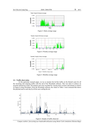
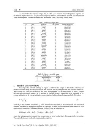
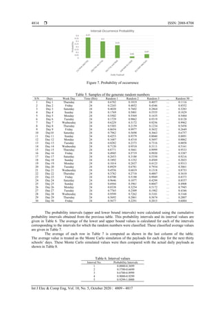
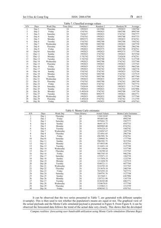
Monte Carlo based simulation model is effective in forecasting the payload internet usage of the study
campus area network. The statistical data used for this study was generated for 50 users for 30 school days.
On average, the total amount of data required to meet the network demand of the user in a month is estimated
as 7.64 gigabytes. Therefore, the total amount of data required to cater to the need of 2500 students in
the campus is estimated as 382 gigabytes.
Figure 8. Actual and Monte Carlo forecast
4. CONCLUSION
The aim of this research work which is to forecast user bandwidth utilization on a campus network
has been largely met. The research used Nuhu Bamalli Polytechnic, Zaria, Kaduna State, Nigeria as a case
study. A network of 50 users concurrently surfing various sites for 30 days was set up with for collecting
data. Monte Carlo simulation was used to forecast user bandwidth utilization to plan campus network design
and capacity upgrade for 2500 users and beyond.
ACKNOWLEDGEMENTS
The authors of this research work will like to take this opportunity to express their gratitude to
the Tertiary Education Trust Fund (TetFund) Institution Based Research for funding this research.
REFERENCES
[1] E. Harstead and R. Sharpe, “Forecasting of access network bandwidth demands for aggregated subscribers using
Monte Carlo methods,” IEEE Communications Magazine, vol. 53, no. 3, pp. 199-207, 2015.
[2] B. Mikavica, V. Radojičić, and A. Kostić-Ljubisavljević, “Estimation of optical access network bandwidth
demand using Monte Carlo simulation,” International Journal for Traffic and Transport Engineering, vol. 5, no. 4,
pp. 384-399, 2015.
[3] S. R. Talpur and T. Kechadi, “A Forecasting Model for Data Center Bandwidth Utilization,” in Proceedings of SAI
Intelligent Systems Conference, pp. 315-330, 2016.
[4] Alaknantha Eswaradass, Xian-He Sun, and Ming Wu, “Network bandwidth predictor (nbp): A system for online
network performance forecasting,” Sixth IEEE International Symposium on Cluster Computing and the Grid,
CCGRID 06, vol. 1, pp. 1-4, 2006.
[5] B. Krithikaivasan, K. Deka, and D. Medhi, “Adaptive Bandwidth Provisioning based on Discrete Temporal
Network Measurements”, in IEEE INFOCOM 04, Hong Kong, China, pp. 1786–1796, 2004.
[6] C. Xiang, P. Qu, and X. Qu, “Network Traffic Prediction Based on MKSVR,” Journal of Information &
Computational Science, pp. 3185–3197, 2015.
[7] G. Booker, et al., “Efficient availability evaluation for transport backbone networks,” in Proceedings of International
Conference on Optical Network Design and Modeling (ONDM), pp. 1-6, 2008. Doi: 10.1109/ONDM.2008.4578386.
[8] Y. Song and F. A. Kuipers, “Traffic Uncertainty Models in Network Planning,” IEEE Communications Magazine,
vol. 52, no. 2, pp. 172-177, 2014. Doi: 10.1109/MCOM.2014.6736759.

9. Int J Elec & Comp Eng ISSN: 2088-8708 
Campus realities: forecasting user bandwidth utilization using Monte Carlo simulation (Haruna Bege)
4817
[9] W. Yoo and A. Sim, “Network bandwidth utilization forecast model on high bandwidth networks,” in 2015
International Conference on Computing, Networking and Communications (ICNC), pp. 494-498, 2015.
[10] N. Rana, K. P. Bhandari, and S. J. Shrestha, “Network Bandwidth Utilization Prediction Based on Observed SNMP
Data,” Journal of the Institute of Engineering, vol. 13, no. 1, pp. 160-168, 2017.
[11] S. Arora and B. S. Brinkman, “A randomized online algorithm for bandwidth utilization,” Journal of Scheduling,
vol. 7, no. 3, pp.187-194, 2004.
[12] D. N. Thaba, “A Framework for optimizing internet bandwidth utilization a Kenyan perspective,” Thesis,
Strathmore University, 2008. [Online]. Available: https://su-plus.strathmore.edu/handle/11071/1477
[13] M. E. Ekpenyong and P. J. Udoh, “Modeling the Effect of Bandwidth Allocation on Network Performance,”
Science World Journal, vol. 9, no. 4, pp. 12-22, 2014.
[14] L. Zhao, et al., “A Filtering Mechanism to Reduce Network Bandwidth Utilization of Transaction Execution,”
ACM Transactions on Architecture and Code Optimization (TACO), vol. 12, no. 4, pp. 1-26, 2016.
[15] R. F. Reale, W. Neto, and J. S. Martins, “AllocTC-sharing: A new bandwidth allocation model for DS-TE
networks,” in 2011 7th Latin American Network Operations and Management Symposium, pp. 1-4, 2011.
[16] S. M. Hasan, M. A. Sahib, A. T. Namel, “Bandwidth Utilization Prediction in LAN Network Using Time
Series Modeling,” Iraqi journal of Computers, Communication, Control, and Systems Engineering, vol. 19, no. 2,
pp. 78-89, 2019.
[17] Y. Li, et al., “Optimization of Bandwidth Utilization in Data Center Network with SDN,” in 2017 2nd International
Conference on Automation, Mechanical Control and Computational Engineering (AMCCE 2017), 2017.
[18] E. Eldesouky, et al., “A Hybrid Cooperative Model for Bandwidth Utilization in Vehicular Ad hoc Networks Based
on Game Theory,” International Journal of Control and Automation, vol. 7, no. 12, pp. 177-188, 2014.
[19] A. Johnson, “Modeling, Implementation, and Evaluation of IP Network Bandwidth Measurement Methods,”
Doctoral thesis, Institutionen för datavetenskap och Elektronik, 2007.
[20] R. K. Paredes and A. A. Hernandez, “Designing an Adaptive Bandwidth Management for Higher Education
Institutions,” International Journal of Computing Sciences Research, vol. 2, no. 1, pp. 17-35, 2018.
[21] M. Kassim, et al., “Bandwidth Control Algorithm on YouTube Video Traffic in Broadband Network,” ournal of
Telecommunication, Electronic and Computer Engineering (JTEC), vol. 10, no. 1-5, pp. 151-156, 2018.
[22] M. Kassim, M. Ismail, and M. I. Yusof, “A New Adaptive Throughput Policy Algorithm on Campus
Ip-Based Network Internet Traffic,” Journal of Theoretical and Applied Information Technology, vol. 71,
no. 2, pp. 205-214, 2015.
[23] O. M. Olanrewaju, “The Modeling and Simulation of Wireless Campus Network,” International Journal of
Computer Science & Information Security, vol. 16, no. 9, 2018.
[24] L. Chitanana, and D. W. Govender, “Bandwidth management in the era of brings your own device,” The Electronic
Journal of Information Systems in Developing Countries, vol. 68, no. 1, pp. 1-14, 2015.
[25] E. A. Noughabi, B. H. Far, and B. Raahemi, “Predicting students’ behavioral patterns in university networks for
efficient bandwidth allocation: A hybrid data mining method,” in IEEE 17th International Conference on
Information Reuse and Integration (IRI), Pittsburgh, PA, USA, 2016. Doi:10.1109/iri.2016.21.
BIOGRAPHIES OF AUTHORS
Haruna Bege is a lecturer at the department of Computer Engineering technology, Nuhu
Bamalli Polytechnic Zaria undergoing his Meng. Electronics and Communications Engineering
at the Nigerian Defence Academy, Kaduna. He obtained his Bachelor’s Degree in
Electrical/Electronic Engineering from Abubakar Tafawa Balewa University, Bauchi, Nigeria.
His research interest is in fields of electronics, communication systems and computer networks.
He is affiliated with Nigeria society of Engineers
Aminu Yusuf Zubairu is a lecturer in the department of Computer Engineering
Technology Nuhu Bamalli Polytechnic Zaria with and Msc Control and Instrumentation from
the University of Derby, United Kingdom. He obtained his bachelor’s degree from Ahmadu
Bello University Zaria in Electrical Enginering. His research interest is in fields of electronics,
control systems, computer technology and artificial intelligence. He is affliated with the Council
for the Reguations of Engineers in Nigeria