How to Doxtabond2
How to Do xtabond2
David Roodman
David Roodman
Research Fellow
Research Fellow
Center for Global Development
Center for Global Development
2.
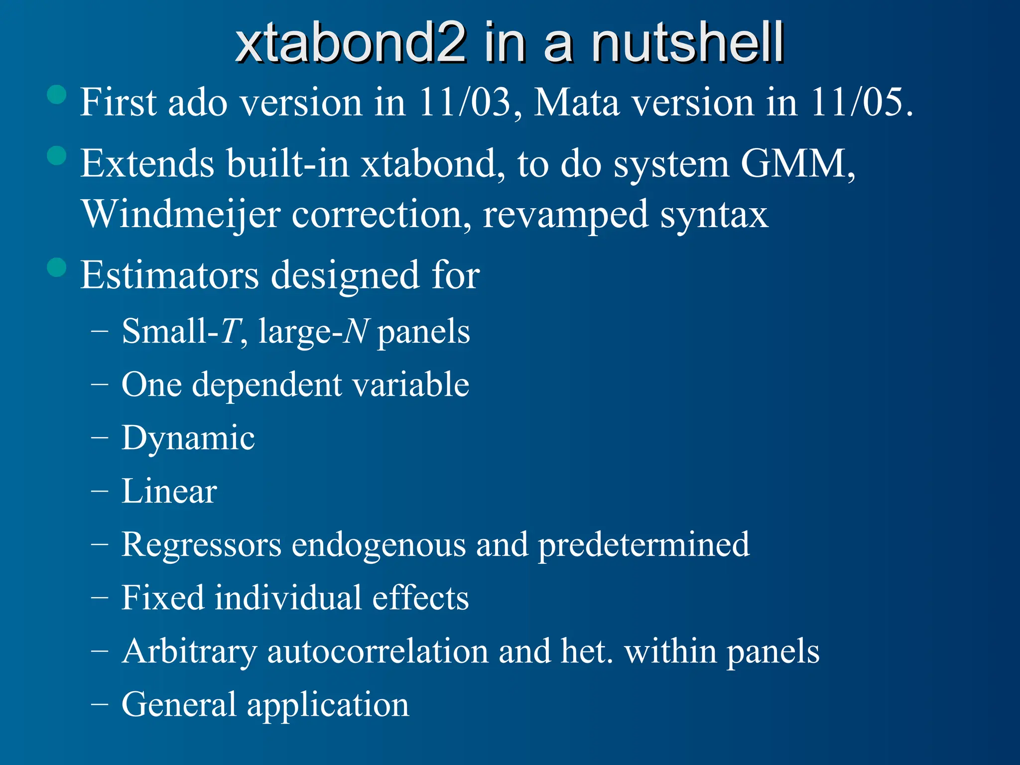
xtabond2 in anutshell
xtabond2 in a nutshell
First ado version in 11/03, Mata version in 11/05.
Extends built-in xtabond, to do system GMM,
Windmeijer correction, revamped syntax
Estimators designed for
– Small-T, large-N panels
– One dependent variable
– Dynamic
– Linear
– Regressors endogenous and predetermined
– Fixed individual effects
– Arbitrary autocorrelation and het. within panels
– General application
3.
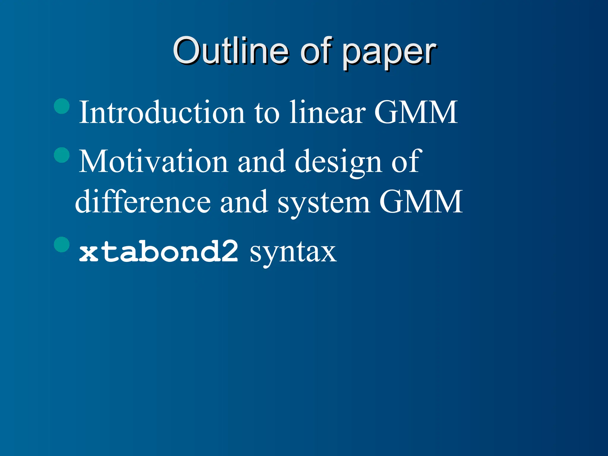
Outline of paper
Outlineof paper
Introduction to linear GMM
Motivation and design of
difference and system GMM
xtabond2 syntax
4.
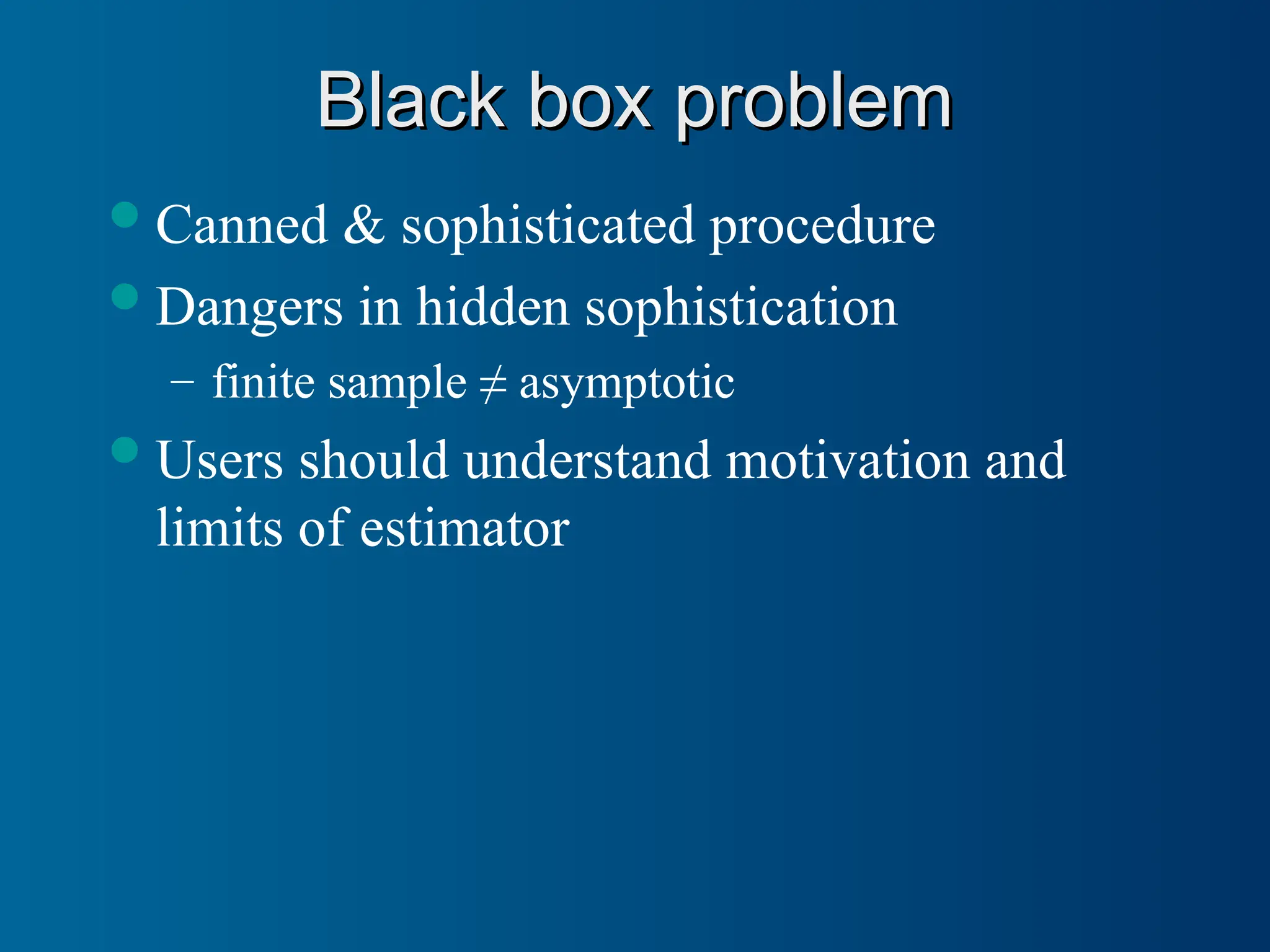
Black box problem
Blackbox problem
Canned & sophisticated procedure
Dangers in hidden sophistication
– finite sample ≠ asymptotic
Users should understand motivation and
limits of estimator
5.
Linear GMM inone slide
Linear GMM in one slide
Instrument vector z such that 0
z
]
E[
# instruments > # parameters so can’t have 0
E
Z
z
ˆ
]
[
E '
1
N
N
Want to “minimize” E
Z ˆ
'
1
N in some sense
In what sense? By a pos-semi-def. quad. form given by A:
E
ZAZ
E
E
Z
A
E
Z
E
Z
z
A
A
ˆ
ˆ
1
ˆ
1
ˆ
1
ˆ
1
E '
'
'
'
'
'
N
N
N
N
N
N
Given A, minimizing leads to Y
ZAZ
X
X
ZAZ
X
A
'
'
1
'
'
ˆ
β
Always unbiased, but which A is efficient? Answer: A should weight
moments E
z'
i inversely with their variances and
covariances:
1
'
1
'
1
'
,
Var
,
Var
Z
Ω
Z
Z
Z
X
E
Z
Z
X
E
Z
AEGMM
To make feasible, choose arbitrary proxy for ,
Ω call it H. Do GMM
(one-step). Use residuals to make robust sandwich estimator of
1
'
Z
Ω
Z . Rerun. Two-step is feasible, theoretically efficient.
6.
Linear GMM and2SLS
Linear GMM and 2SLS
Y
Z
Z
Ω
Z
Z
X
X
Z
Z
Ω
Z
Z
X '
1
'
'
1
'
1
'
'
ˆ
EGMM
β
If ,
2
I
Ω
reduces to
Y
Z
Z
Z
Z
X
X
Z
Z
Z
Z
X '
1
'
'
1
'
1
'
'
2
ˆ
SLS
β
If errors i.i.d., efficient GMM is 2SLS
If not, 2SLS inefficient
7.
Linear GMM inanother slide
Linear GMM in another slide
(Holtz-Eakin, Newey, and Rosen 1988)
(Holtz-Eakin, Newey, and Rosen 1988)
(1) E
X
Y
β
OLS inconsistent: 0
E '
E
X
(2) Take Z-moments: E
Z
X
Z
Y
Z '
'
'
β
OLS consistent
0
'
E '
E
ZZ
X
but inefficient
scalar
not
'
'
Var ΩZ
Z
E
Z
Left-multiply by 2
1
'
ΩZ
Z :
E
Z
ΩZ
Z
X
Z
ΩZ
Z
Y
Z
ΩZ
Z '
2
1
'
'
2
1
'
'
2
1
'
β
Let ,
'
2
1
'
*
X
Z
ΩZ
Z
X
,
'
2
1
'
*
Y
Z
ΩZ
Z
Y
E
Z
ΩZ
Z
E '
2
1
'
*
(3)
*
*
*
E
X
Y
β
OLS efficient
I
E
Var *
OLS on (3) = GLS on (2) = GMM on (1)
GMM = GLS on Z-moments
8.
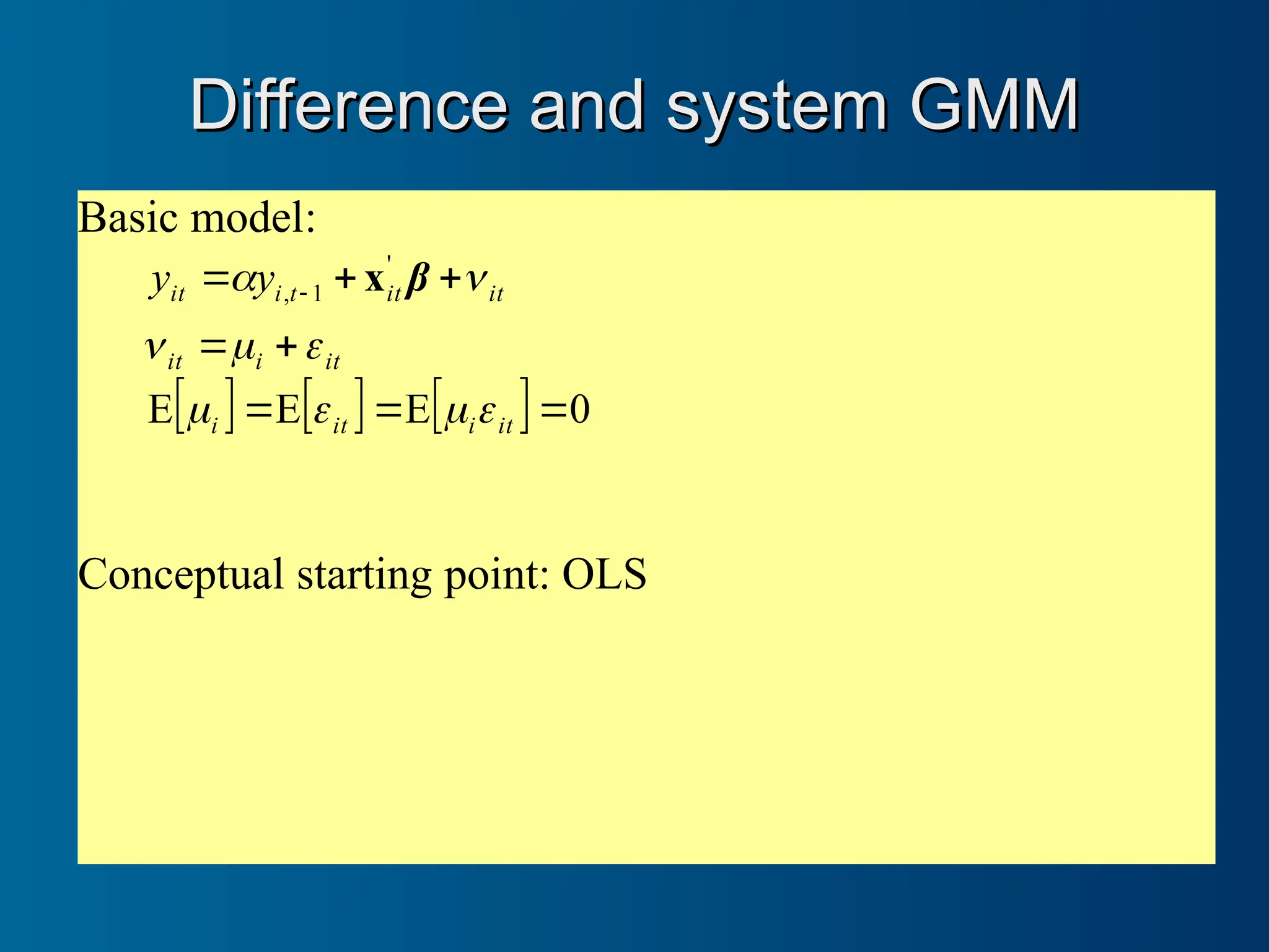
Difference and systemGMM
Difference and system GMM
Basic model:
0
E
E
E
'
1
,
it
i
it
i
it
i
it
it
it
t
i
it y
y
β
x
Conceptual starting point: OLS
9.
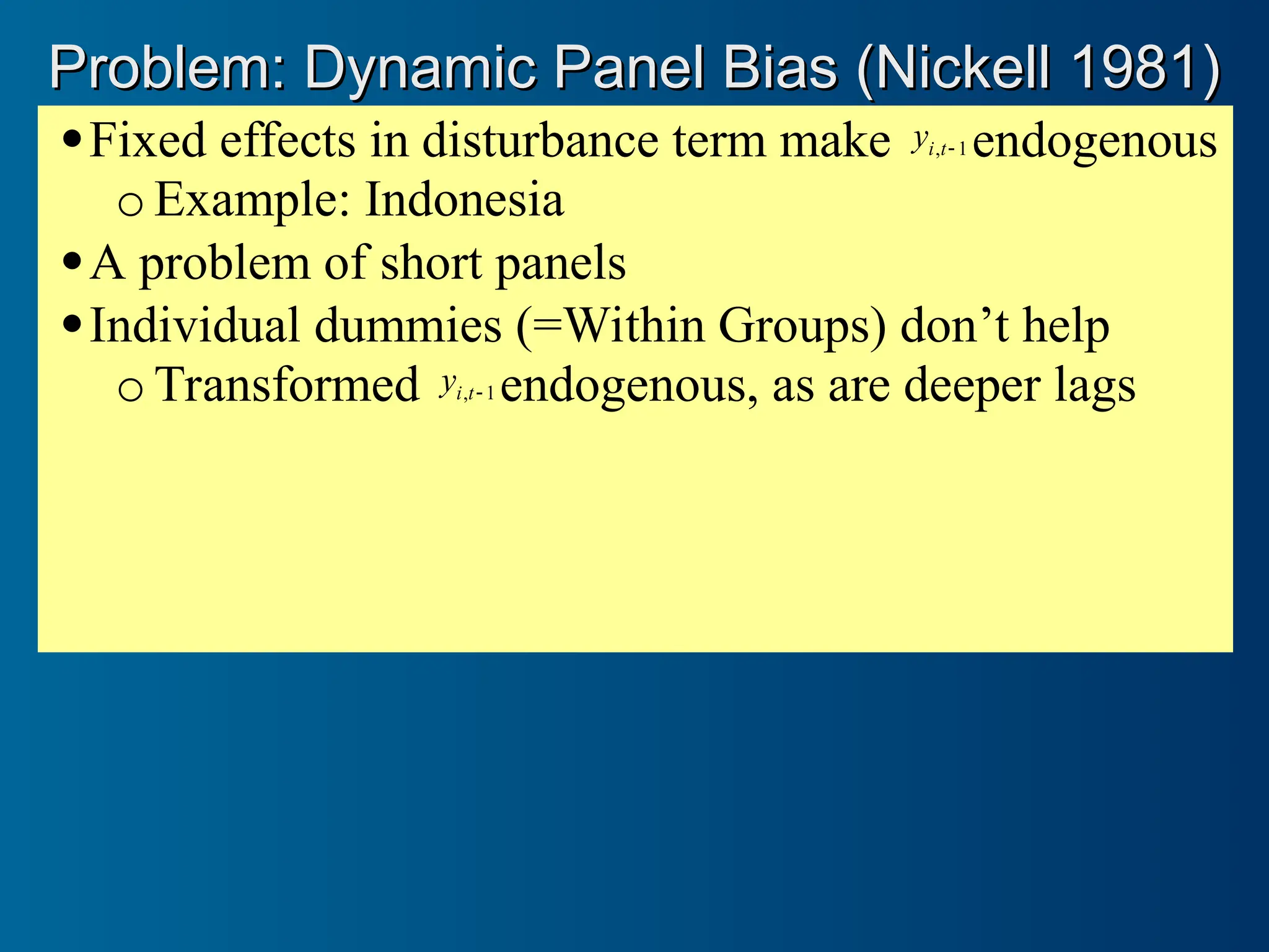
Fixed effects indisturbance term make 1
,
t
i
y endogenous
o Example: Indonesia
A problem of short panels
Individual dummies (=Within Groups) don’t help
o Transformed 1
,
t
i
y endogenous, as are deeper lags
Problem: Dynamic Panel Bias (Nickell 1981)
Problem: Dynamic Panel Bias (Nickell 1981)
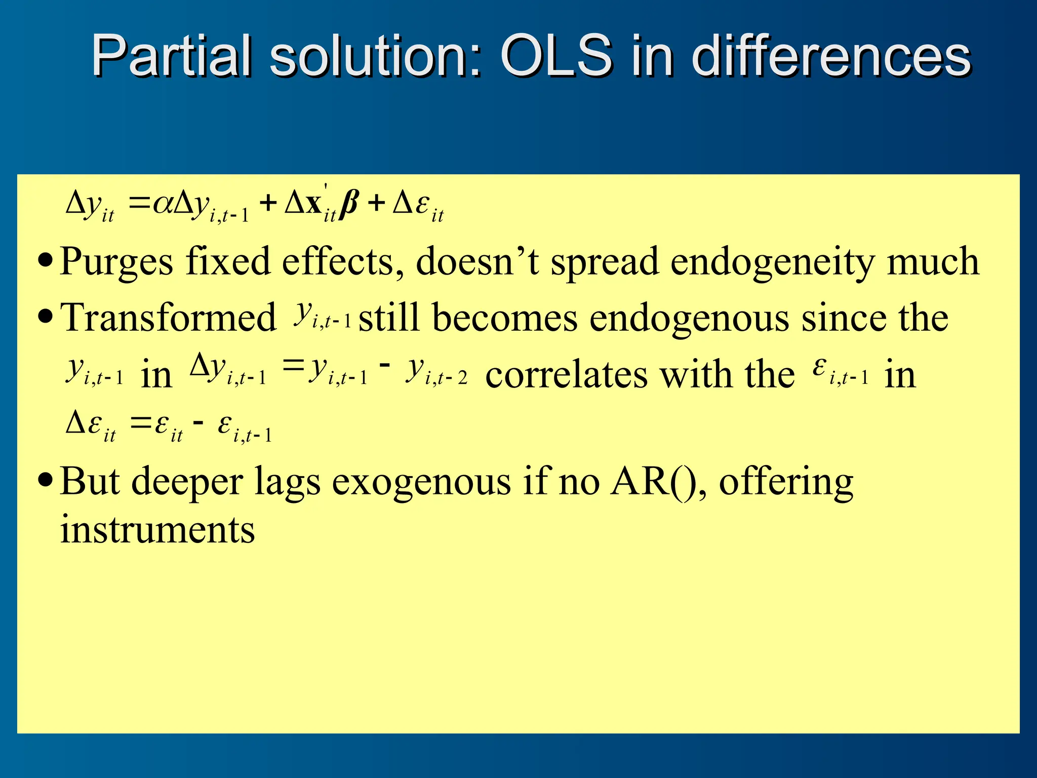
10.
it
it
t
i
it y
y
β
'
1
, x
Purges fixed effects, doesn’t spread endogeneity much
Transformed 1
,
t
i
y still becomes endogenous since the
1
,
t
i
y in 2
,
1
,
1
,
t
i
t
i
t
i y
y
y correlates with the 1
,
t
i
in
1
,
t
i
it
it
But deeper lags exogenous if no AR(), offering
instruments
Partial solution: OLS in differences
Partial solution: OLS in differences
11.
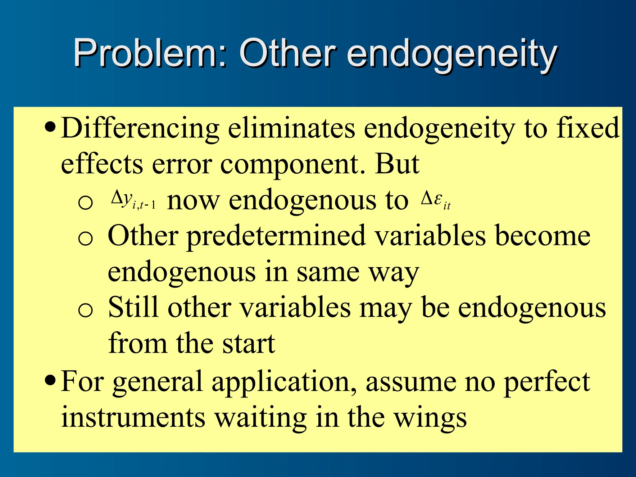
Differencing eliminates endogeneityto fixed
effects error component. But
o 1
,
t
i
y now endogenous to it
o Other predetermined variables become
endogenous in same way
o Still other variables may be endogenous
from the start
For general application, assume no perfect
instruments waiting in the wings
Problem: Other endogeneity
Problem: Other endogeneity
12.
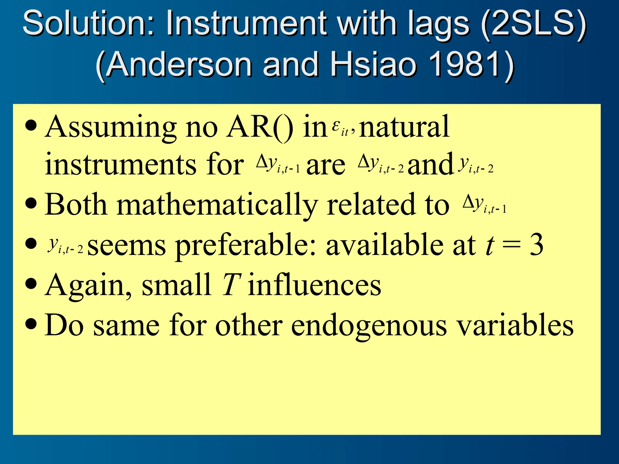
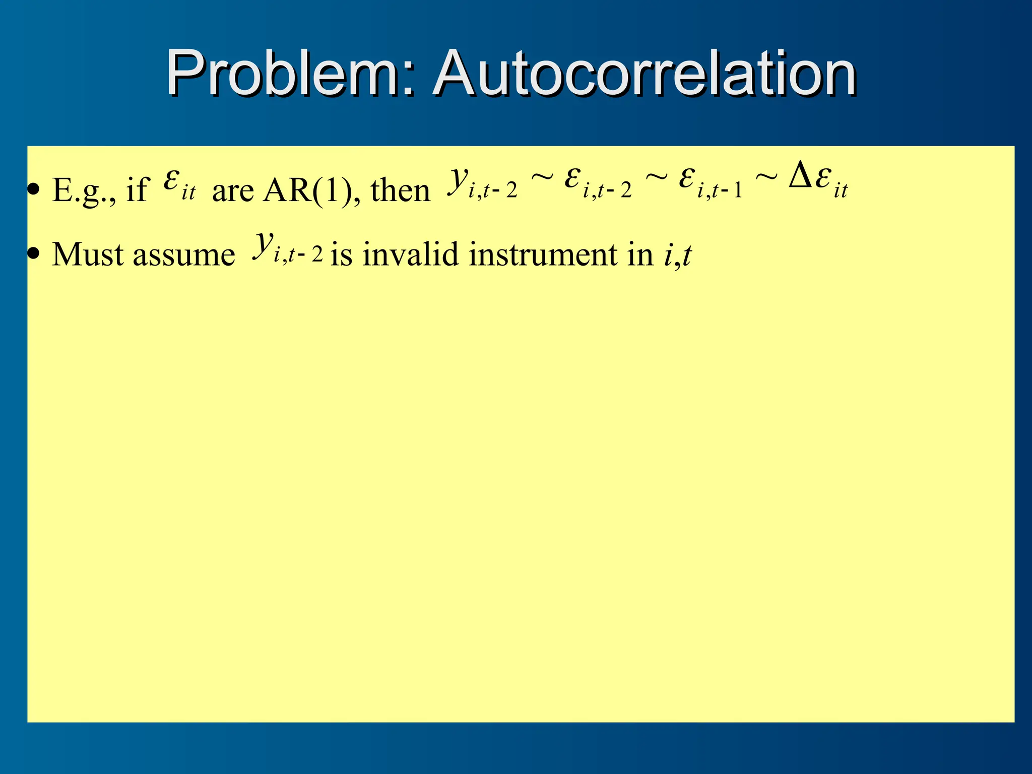
Assuming noAR() in ,
it
natural
instruments for 1
,
t
i
y are 2
,
t
i
y and 2
,
t
i
y
Both mathematically related to 1
,
t
i
y
2
,
t
i
y seems preferable: available at t = 3
Again, small T influences
Do same for other endogenous variables
Solution: Instrument with lags (2SLS)
Solution: Instrument with lags (2SLS)
(Anderson and Hsiao 1981)
(Anderson and Hsiao 1981)
13.
Deeper lags availableas instruments
o But reduce sample in 2SLS
o Problem for short panels
In differences, errors not i.i.d.
o it
and 1
,
t
i
mathematically correlated
o 2SLS not efficient
Problem: Inefficiency
Problem: Inefficiency
14.
Use many lags,replacing missing with zero
Generate separate instrument for each lag and time
period instrumented
IV-style:
2
,
1
.
.
T
i
i
y
y
GMM-style:
.
0
0
0
0
0
0
0
0
0
0
0
0
0
0
0
0
0
0
0
0
0
0
0
0
1
2
3
1
2
1
i
i
i
i
i
i
y
y
y
y
y
y
Result: Arellano-Bond (1991) difference GMM
Solution: GMM & GMM-style instruments
Solution: GMM & GMM-style instruments
(Holtz-Eakin, Newey, and Rosen 1988)
(Holtz-Eakin, Newey, and Rosen 1988)
15.
E.g., ifit
are AR(1), then it
t
i
t
i
t
i
y
~
~
~ 1
,
2
,
2
,
Must assume 2
,
t
i
y is invalid instrument in i,t
Problem: Autocorrelation
Problem: Autocorrelation
16.
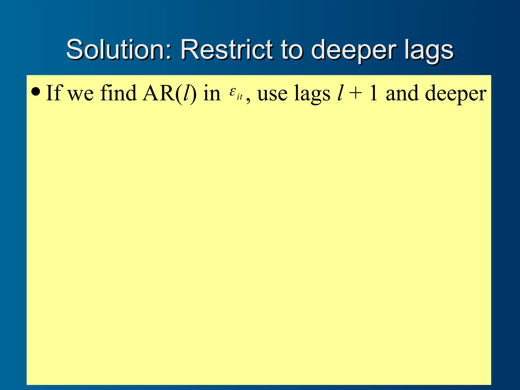
If wefind AR(l) in it
, use lags l + 1 and deeper
Solution: Restrict to deeper lags
Solution: Restrict to deeper lags
17.
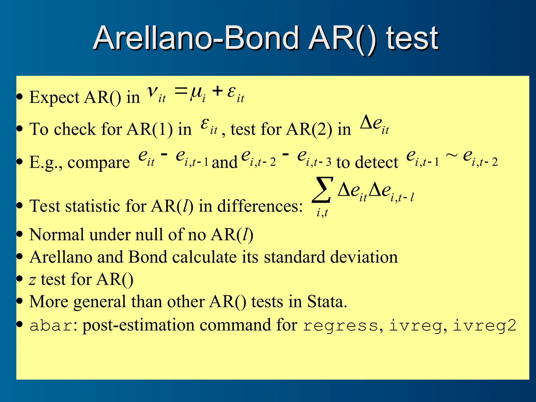
Expect AR()in it
i
it
To check for AR(1) in it
, test for AR(2) in it
e
E.g., compare 1
,
t
i
it e
e and 3
,
2
,
t
i
t
i e
e to detect 2
,
1
, ~
t
i
t
i e
e
Test statistic for AR(l) in differences:
t
i
l
t
i
it e
e
,
,
Normal under null of no AR(l)
Arellano and Bond calculate its standard deviation
z test for AR()
More general than other AR() tests in Stata.
abar: post-estimation command for regress, ivreg, ivreg2
Arellano-Bond AR() test
Arellano-Bond AR() test
18.
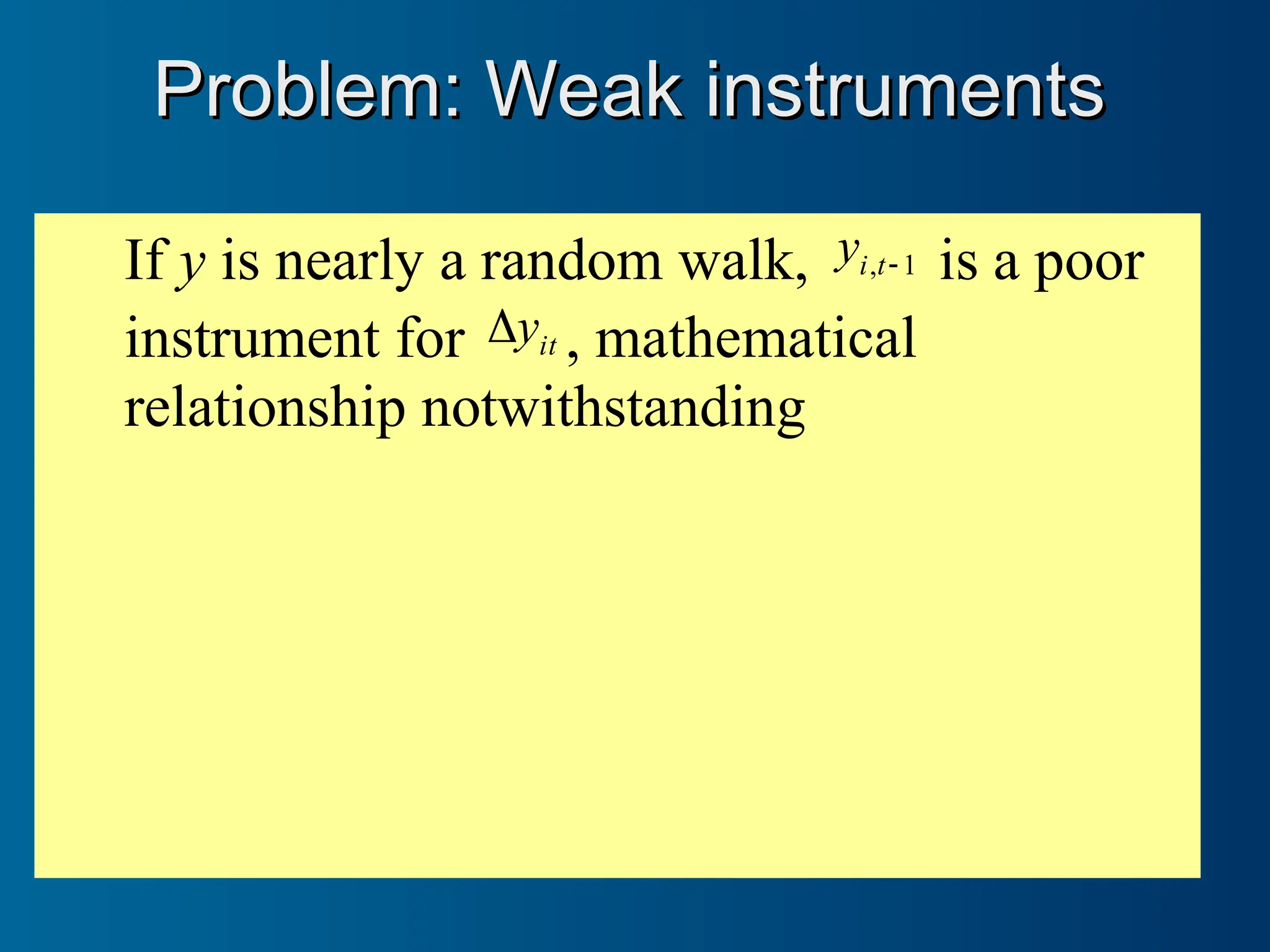
If y isnearly a random walk, 1
,
t
i
y is a poor
instrument for it
y
, mathematical
relationship notwithstanding
Problem: Weak instruments
Problem: Weak instruments
19.
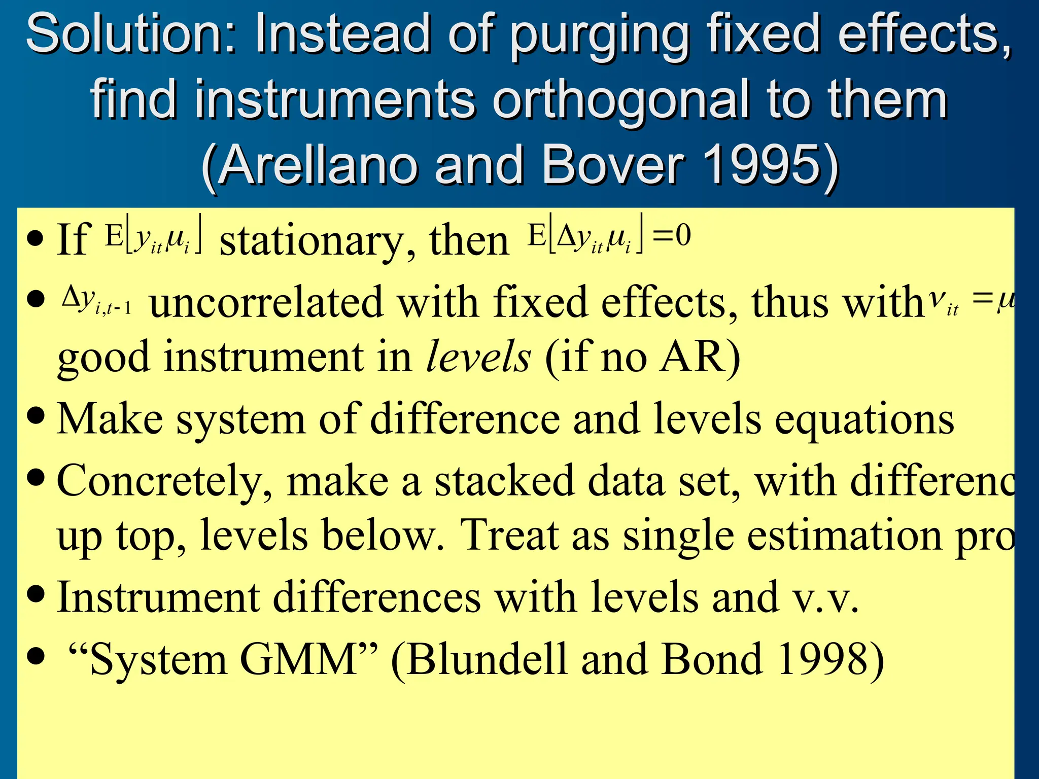
If
i
it
y
E stationary, then 0
E
i
it
y
1
,
t
i
y uncorrelated with fixed effects, thus with i
it
good instrument in levels (if no AR)
Make system of difference and levels equations
Concretely, make a stacked data set, with difference
up top, levels below. Treat as single estimation prob
Instrument differences with levels and v.v.
“System GMM” (Blundell and Bond 1998)
Solution: Instead of purging fixed effects,
Solution: Instead of purging fixed effects,
find instruments orthogonal to them
find instruments orthogonal to them
(Arellano and Bover 1995)
(Arellano and Bover 1995)
20.
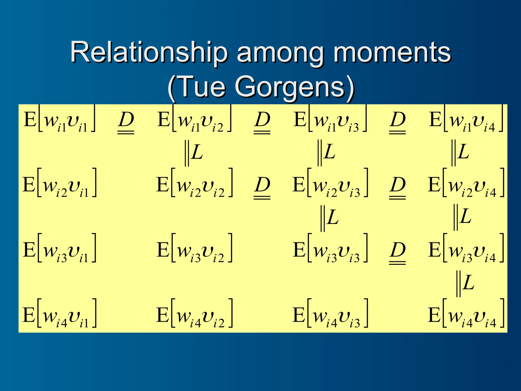
4
4
3
4
2
4
1
4
4
3
3
3
2
3
1
3
4
2
3
2
2
2
1
2
4
1
3
1
2
1
1
1
E
E
E
E
E
E
E
E
E
E
E
E
E
E
E
E
i
i
i
i
i
i
i
i
i
i
i
i
i
i
i
i
i
i
i
i
i
i
i
i
i
i
i
i
i
i
i
i
w
w
w
w
L
w
D
w
w
w
L
w
D
w
D
w
w
L
w
D
w
D
w
D
w
Relationship among moments
Relationship among moments
(Tue Gorgens)
(Tue Gorgens)
L
L
L
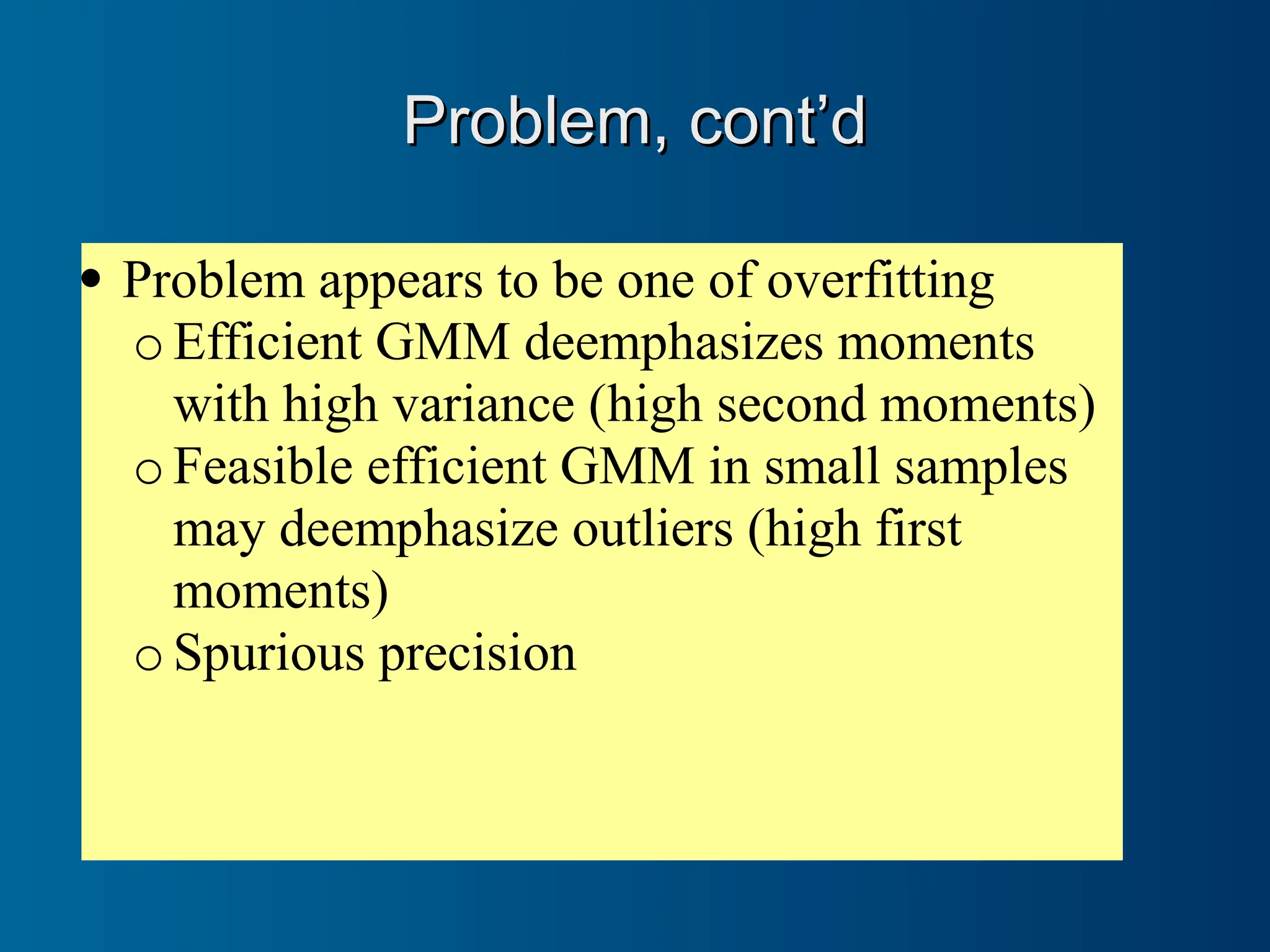
Problem appearsto be one of overfitting
o Efficient GMM deemphasizes moments
with high variance (high second moments)
o Feasible efficient GMM in small samples
may deemphasize outliers (high first
moments)
o Spurious precision
Problem, cont’d
Problem, cont’d
23.
oOne-step estimate:
Y
f
1
β̂ (conditioning on X, Z)
oOne-step residuals used to constructΩ̂ :
))
(
,
(
)
ˆ
,
(
ˆ
ˆ
ˆ '
1
'
'
1
'
1
'
'
2 Y
Y
Ω
Y
Y
Z
Z
Ω
Z
Z
X
X
Z
Z
Ω
Z
Z
X f
g
g
β
oStandard estimate of
2
ˆ
Var β treats Ω̂ as constant,
observed, precise—despite dependence on random Y
oTaylor expansion of g around true β :
β
β
β
β
β
β
1
ˆ
ˆ
ˆ
2
ˆ
ˆ
,
ˆ
ˆ
,
ˆ
,
ˆ
1
Ω
Y
Ω
Y
Ω
Y g
g
g
o“Correction” comes from second term
0
ˆ
E 1
β
β so no effect on
2
ˆ
E β —no coefficient bias
Affects variance
Solution: finite-sample correction
Solution: finite-sample correction
(Windmeijer 2005)
(Windmeijer 2005)
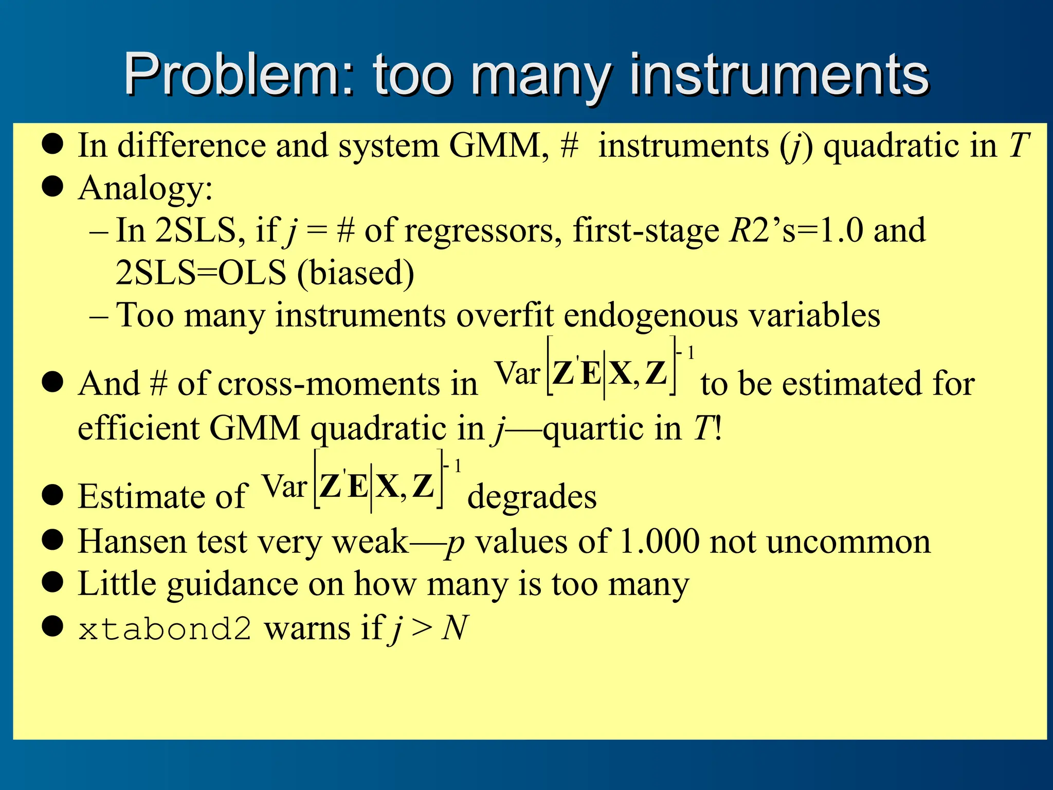
Problem: too manyinstruments
Problem: too many instruments
In difference and system GMM, # instruments (j) quadratic in T
Analogy:
– In 2SLS, if j = # of regressors, first-stage R2’s=1.0 and
2SLS=OLS (biased)
– Too many instruments overfit endogenous variables
And # of cross-moments in 1
'
,
Var
Z
X
E
Z to be estimated for
efficient GMM quadratic in j—quartic in T!
Estimate of 1
'
,
Var
Z
X
E
Z degrades
Hansen test very weak—p values of 1.000 not uncommon
Little guidance on how many is too many
xtabond2 warns if j > N
26.
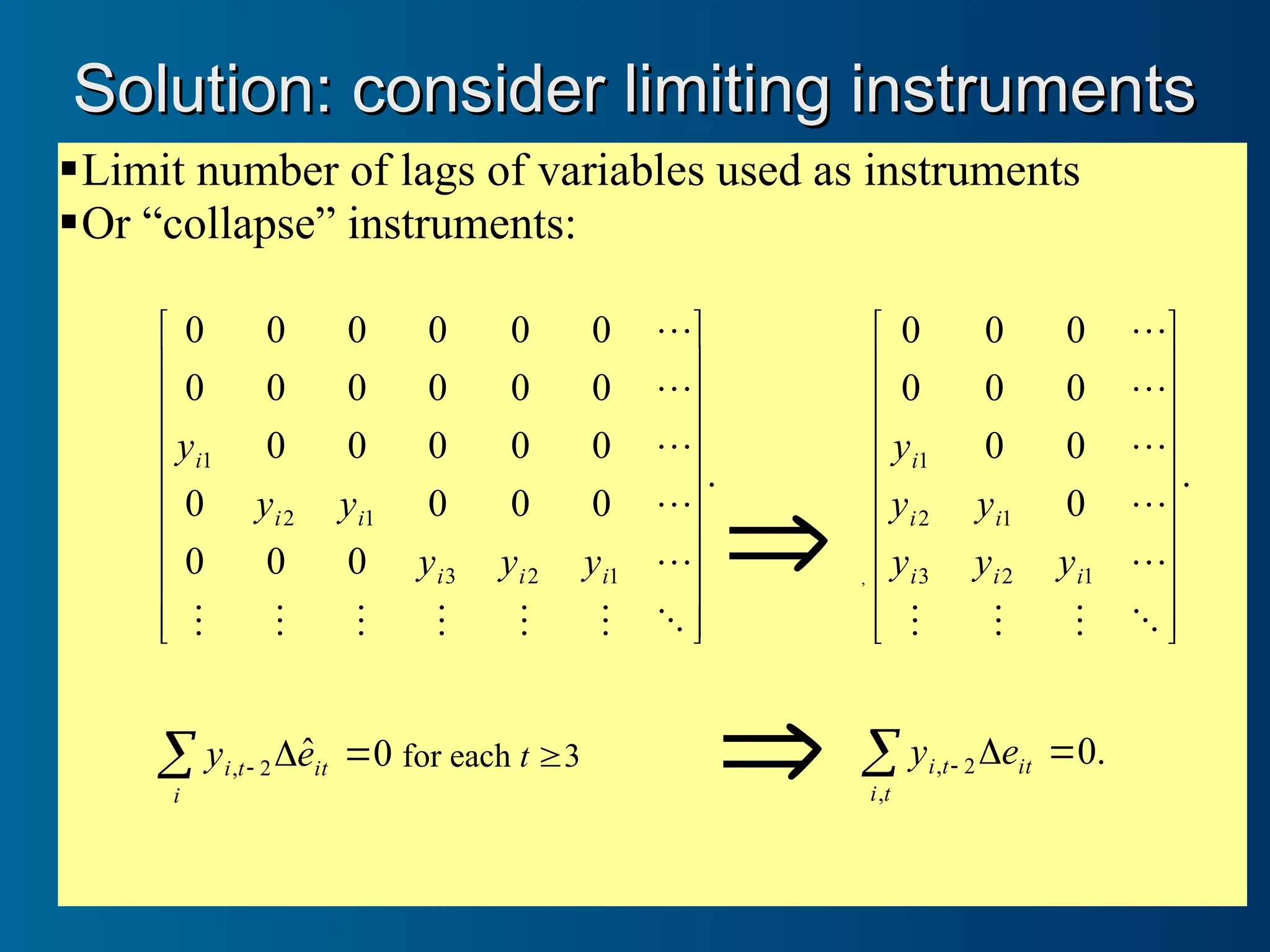
Limit number oflags of variables used as instruments
Or “collapse” instruments:
.
0
0
0
0
0
0
0
0
0
0
0
0
0
0
0
0
0
0
0
0
0
0
0
0
1
2
3
1
2
1
i
i
i
i
i
i
y
y
y
y
y
y
,
.
0
0
0
0
0
0
0
0
0
1
2
3
1
2
1
i
i
i
i
i
i
y
y
y
y
y
y
0
ˆ
2
,
it
i
t
i e
y for each t 3
.
0
,
2
,
it
t
i
t
i e
y
Solution: consider limiting instruments
Solution: consider limiting instruments
27.
xtabond2
xtabond2 syntax
syntax
xtabond2 depvarvarlist [if exp] [in range]
[, level(#) twostep robust noconstant small noleveleq
artests(#) arlevels h(#) nomata]
ivopt [ivopt ...] gmmopt [gmmopt ...]]
where gmmopt is
gmmstyle(varlist [, laglimits(# #) collapse
equation({diff | level | both}) passthru])
and ivopt is
ivstyle(varlist [, equation({diff | level | both})
passthru mz])
Y X Z
Classic
“GMM-style”
28.
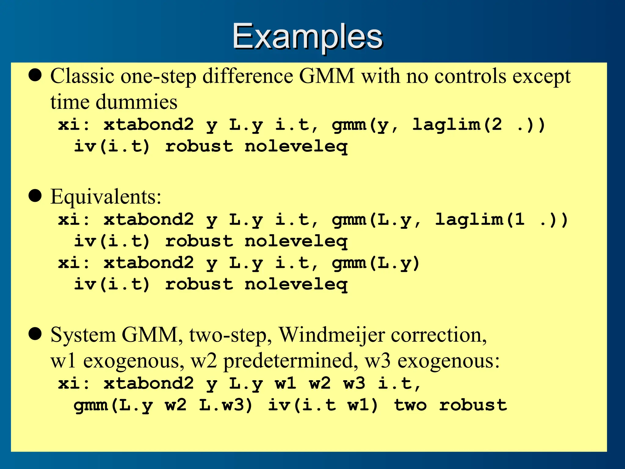
Examples
Examples
Classic one-step differenceGMM with no controls except
time dummies
xi: xtabond2 y L.y i.t, gmm(y, laglim(2 .))
iv(i.t) robust noleveleq
Equivalents:
xi: xtabond2 y L.y i.t, gmm(L.y, laglim(1 .))
iv(i.t) robust noleveleq
xi: xtabond2 y L.y i.t, gmm(L.y)
iv(i.t) robust noleveleq
System GMM, two-step, Windmeijer correction,
w1 exogenous, w2 predetermined, w3 exogenous:
xi: xtabond2 y L.y w1 w2 w3 i.t,
gmm(L.y w2 L.w3) iv(i.t w1) two robust
29.
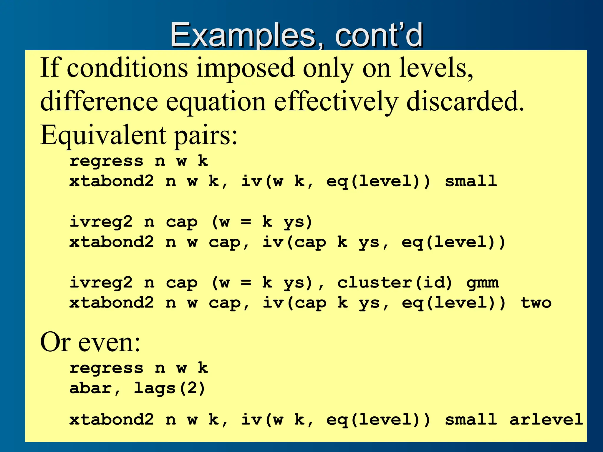
Examples, cont’d
Examples, cont’d
Ifconditions imposed only on levels,
difference equation effectively discarded.
Equivalent pairs:
regress n w k
xtabond2 n w k, iv(w k, eq(level)) small
ivreg2 n cap (w = k ys)
xtabond2 n w cap, iv(cap k ys, eq(level))
ivreg2 n cap (w = k ys), cluster(id) gmm
xtabond2 n w cap, iv(cap k ys, eq(level)) two
Or even:
regress n w k
abar, lags(2)
xtabond2 n w k, iv(w k, eq(level)) small arlevel
30.
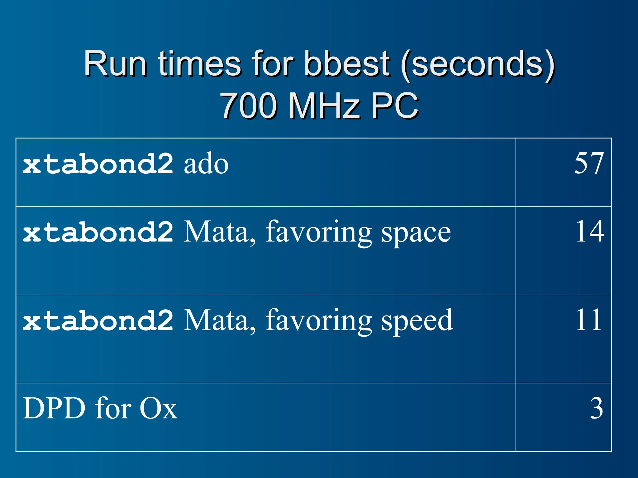
Run times forbbest (seconds)
Run times for bbest (seconds)
700 MHz PC
700 MHz PC
xtabond2 ado 57
xtabond2 Mata, favoring space 14
xtabond2 Mata, favoring speed 11
DPD for Ox 3

![Linear GMM in one slide
Linear GMM in one slide
Instrument vector z such that 0
z
]
E[
# instruments > # parameters so can’t have 0
E
Z
z
ˆ
]
[
E '
1
N
N
Want to “minimize” E
Z ˆ
'
1
N in some sense
In what sense? By a pos-semi-def. quad. form given by A:
E
ZAZ
E
E
Z
A
E
Z
E
Z
z
A
A
ˆ
ˆ
1
ˆ
1
ˆ
1
ˆ
1
E '
'
'
'
'
'
N
N
N
N
N
N
Given A, minimizing leads to Y
ZAZ
X
X
ZAZ
X
A
'
'
1
'
'
ˆ
β
Always unbiased, but which A is efficient? Answer: A should weight
moments E
z'
i inversely with their variances and
covariances:
1
'
1
'
1
'
,
Var
,
Var
Z
Ω
Z
Z
Z
X
E
Z
Z
X
E
Z
AEGMM
To make feasible, choose arbitrary proxy for ,
Ω call it H. Do GMM
(one-step). Use residuals to make robust sandwich estimator of
1
'
Z
Ω
Z . Rerun. Two-step is feasible, theoretically efficient.](https://image.slidesharecdn.com/how2doxtabond2-250630154849-b60c9212/75/Cach-s-d-ng-XTABOND2-trong-STATA-v-i-GMM-5-2048.jpg)
![Problem: Two-step errors too small
Problem: Two-step errors too small
Regression for Arellano-Bond (1991) column (a1), Table 4
Arellano-Bond dynamic panel-data estimation, one-step difference GMM results
------------------------------------------------------------------------------
| Robust
| Coef. Std. Err. t P>|t| [95% Conf. Interval]
-------------+----------------------------------------------------------------
n |
L1. | .6862261 .1445943 4.75 0.000 .4003376 .9721147
L2. | -.0853582 .0560155 -1.52 0.130 -.1961109 .0253944
w |
--. | -.6078208 .1782055 -3.41 0.001 -.9601647 -.2554769
L1. | .3926237 .1679931 2.34 0.021 .0604714 .7247759
k |
--. | .3568456 .0590203 6.05 0.000 .240152 .4735392
Arellano-Bond dynamic panel-data estimation, two-step difference GMM results
------------------------------------------------------------------------------
| Coef. Std. Err. t P>|t| [95% Conf. Interval]
-------------+----------------------------------------------------------------
n |
L1. | .6287089 .0904543 6.95 0.000 .4498646 .8075531
L2. | -.0651882 .0265009 -2.46 0.015 -.1175852 -.0127912
w |
--. | -.5257597 .0537692 -9.78 0.000 -.6320709 -.4194485
L1. | .3112899 .0940116 3.31 0.001 .1254122 .4971675
k |
--. | .2783619 .0449083 6.20 0.000 .1895702 .3671537](https://image.slidesharecdn.com/how2doxtabond2-250630154849-b60c9212/75/Cach-s-d-ng-XTABOND2-trong-STATA-v-i-GMM-21-2048.jpg)
![Arellano-Bond dynamic panel-data estimation, one-step difference GMM results
------------------------------------------------------------------------------
| Robust
| Coef. Std. Err. t P>|t| [95% Conf. Interval]
-------------+----------------------------------------------------------------
n |
L1. | .6862261 .1445943 4.75 0.000 .4003376 .9721147
L2. | -.0853582 .0560155 -1.52 0.130 -.1961109 .0253944
w |
--. | -.6078208 .1782055 -3.41 0.001 -.9601647 -.2554769
L1. | .3926237 .1679931 2.34 0.021 .0604714 .7247759
k |
--. | .3568456 .0590203 6.05 0.000 .240152 .4735392
Arellano-Bond dynamic panel-data estimation, two-step difference GMM results
------------------------------------------------------------------------------
| Coef. Std. Err. t P>|t| [95% Conf. Interval]
-------------+----------------------------------------------------------------
n |
L1. | .6287089 .0904543 6.95 0.000 .4498646 .8075531
L2. | -.0651882 .0265009 -2.46 0.015 -.1175852 -.0127912
w |
--. | -.5257597 .0537692 -9.78 0.000 -.6320709 -.4194485
L1. | .3112899 .0940116 3.31 0.001 .1254122 .4971675
k |
--. | .2783619 .0449083 6.20 0.000 .1895702 .3671537
Arellano-Bond dynamic panel-data estimation, two-step difference GMM results
------------------------------------------------------------------------------
| Corrected
| Coef. Std. Err. t P>|t| [95% Conf. Interval]
-------------+----------------------------------------------------------------
n |
L1. | .6287089 .1934138 3.25 0.001 .2462954 1.011122
L2. | -.0651882 .0450501 -1.45 0.150 -.1542602 .0238838
w |
--. | -.5257597 .1546107 -3.40 0.001 -.8314524 -.2200669
L1. | .3112899 .2030006 1.53 0.127 -.0900784 .7126582
k |
--. | .2783619 .0728019 3.82 0.000 .1344196 .4223043](https://image.slidesharecdn.com/how2doxtabond2-250630154849-b60c9212/75/Cach-s-d-ng-XTABOND2-trong-STATA-v-i-GMM-24-2048.jpg)
![xtabond2
xtabond2 syntax
syntax
xtabond2 depvar varlist [if exp] [in range]
[, level(#) twostep robust noconstant small noleveleq
artests(#) arlevels h(#) nomata]
ivopt [ivopt ...] gmmopt [gmmopt ...]]
where gmmopt is
gmmstyle(varlist [, laglimits(# #) collapse
equation({diff | level | both}) passthru])
and ivopt is
ivstyle(varlist [, equation({diff | level | both})
passthru mz])
Y X Z
Classic
“GMM-style”](https://image.slidesharecdn.com/how2doxtabond2-250630154849-b60c9212/75/Cach-s-d-ng-XTABOND2-trong-STATA-v-i-GMM-27-2048.jpg)