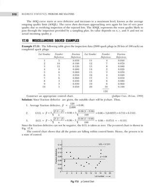
This document provides a summary of a business statistics textbook. It begins with an introduction by the author, J.K. Sharma, who is a former professor of business statistics. The book then covers topics such as data classification, measures of central tendency, probability, sampling, hypothesis testing, correlation and regression analysis. It contains 20 chapters and includes examples and practice problems for readers. The book is published by Dorling Kindersley and aims to help readers understand and solve problems in business statistics.


![9
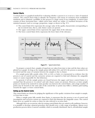
DATA CLASSIFICATION, TABULATION, AND PRESENTATION
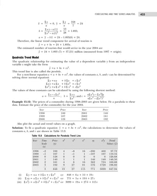
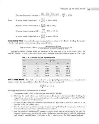
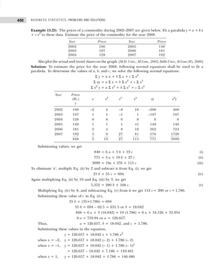
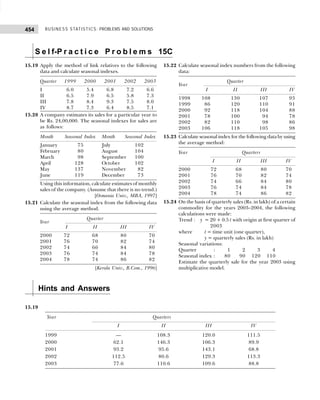
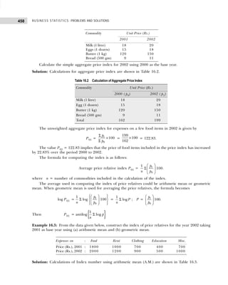
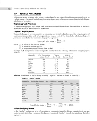
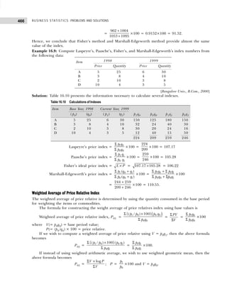
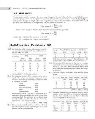
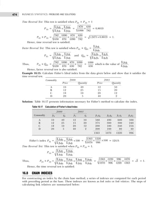
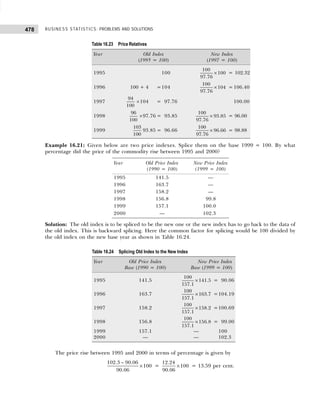
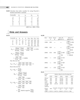
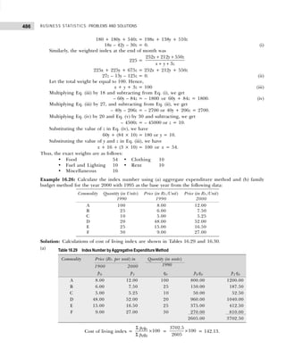
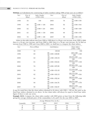
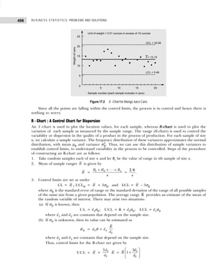
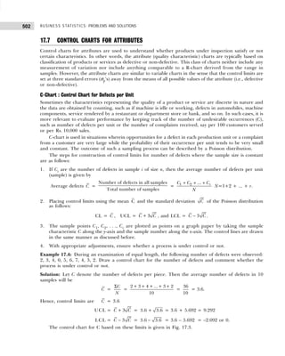
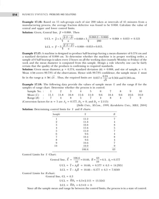
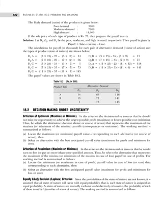
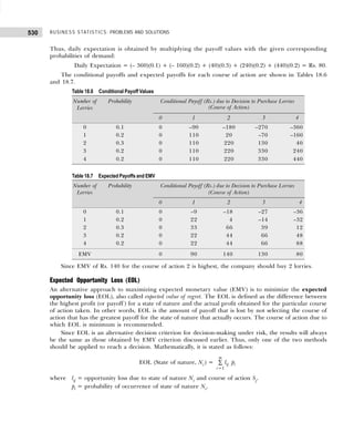
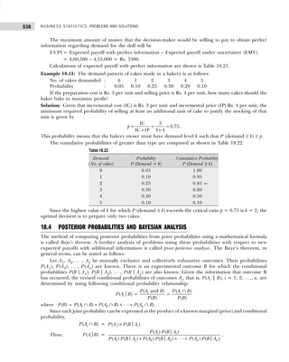
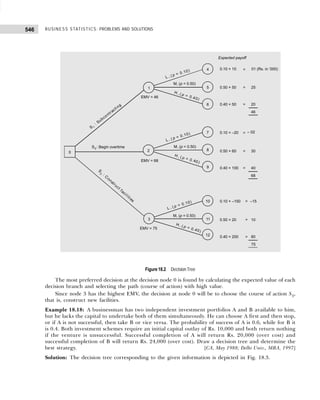
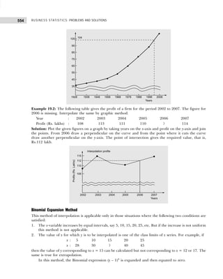
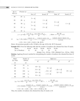
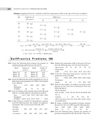
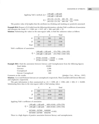
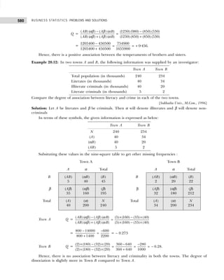
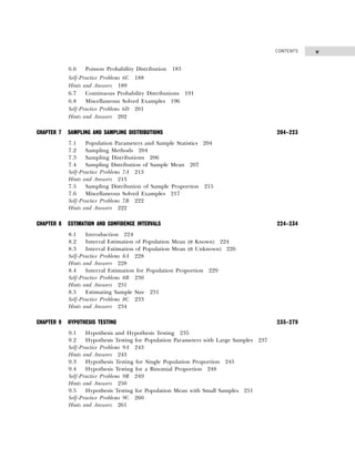
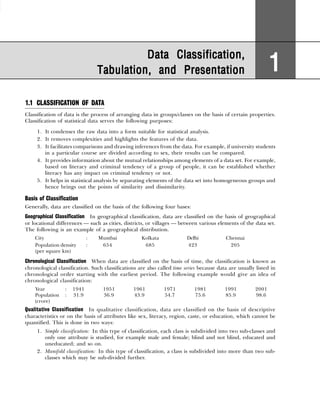
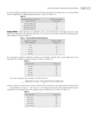
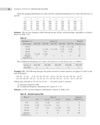
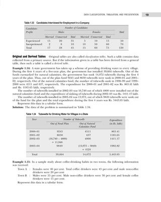
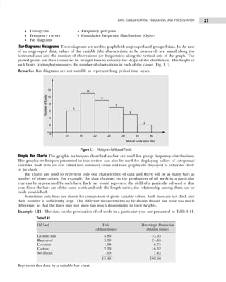
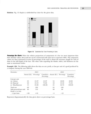
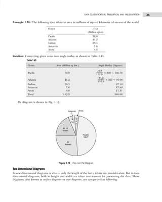
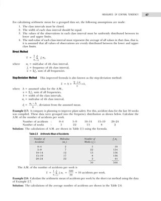
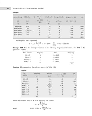
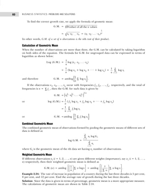
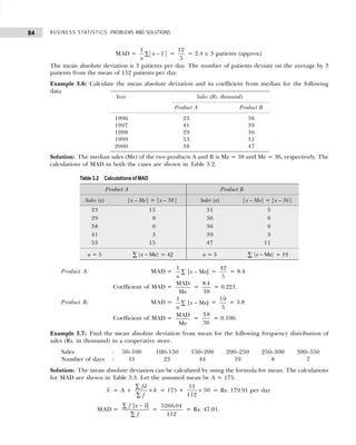
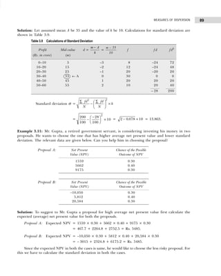
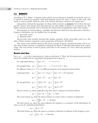
Converting the class intervals shown in Table 1.16 into exclusive class intervals is shown in Table 1.17.
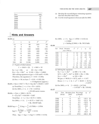
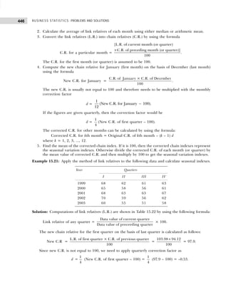
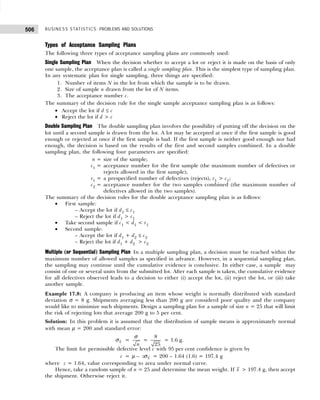
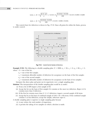
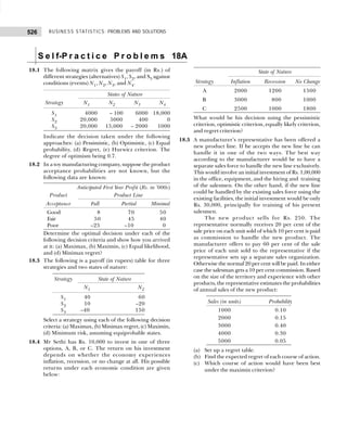
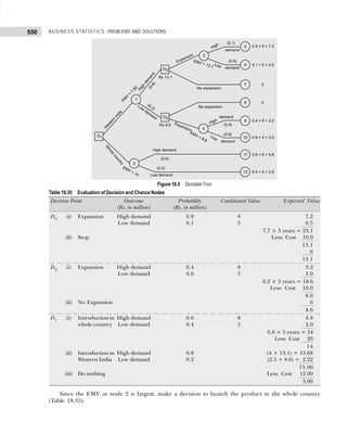
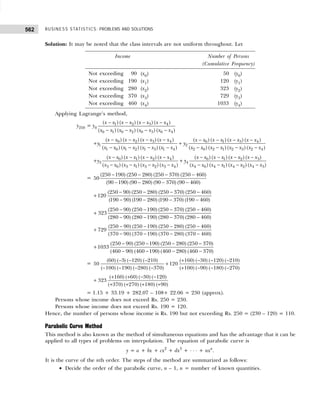
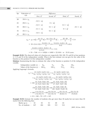
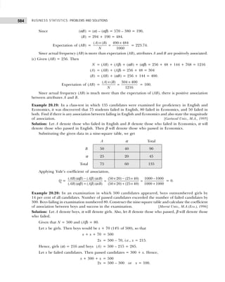
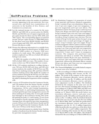
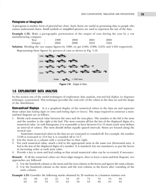
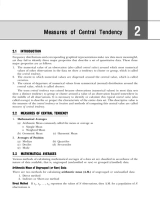
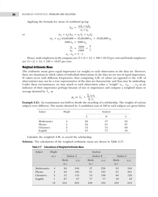
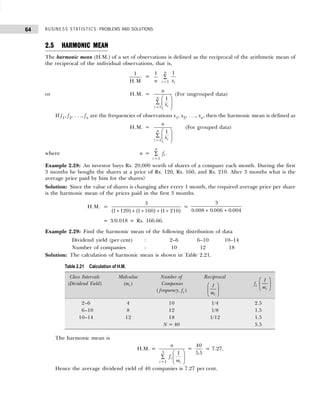
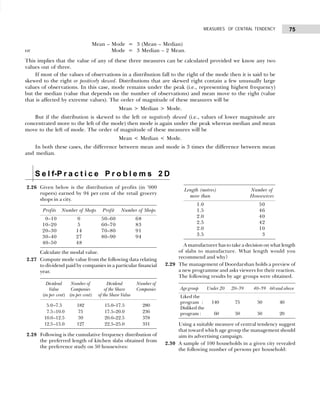
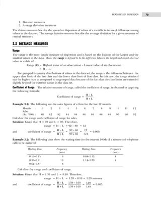
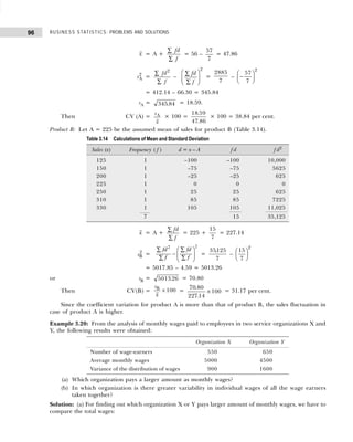
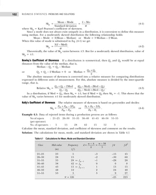
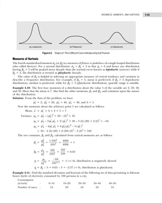
Example 1.6: Classify the following data by taking class such that their mid-values are 17, 22, 27, 32, and
so on.
30 42 30 54 40 48 15 17 51 42 25 41
30 27 42 36 28 26 37 54 44 31 36 40
36 22 30 31 19 48 16 42 32 21 22 46
33 41 21
[Madurai-Kamaraj Univ., B.Com., 2005]
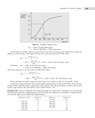
Solution: Since we have to classify the data in such a manner that the mid-values are 17, 22, 27, etc., the
first class should be 15–19 (mid-value = (15 + 19)/2 = 17), second class should be 20–24, etc. Performing
the actual tally and counting the number of observations in each class we get the frequency distribution as
shown in Table 1.18.
Table 1.18 Frequency Distribution with Inclusive Class Intervals
Marks Tallies Frequency
15–19 |||| 4
20–24 |||| 4
25–29 |||| 4
30–34 |||| ||| 8
35–39 |||| 4
40–44 |||| |||| 9
45–49 ||| 3
50–54 ||| 3
39
Table 1.16 Frequency Distribution with Inclusive Class Intervals
Class Intervals Tally Frequency
(Number of Items Produced)
14–17 | | | | | 6
18–21 | | | | | | | | | | | | | | | 18
22–25 | | | | | | | | | | | | 15
26–29 | | | | 5
30–33 | | | 3
34–33 | | | 3
50
Table 1.17 Frequency Distribution with Exclusive Class Intervals
Class Intervals Mid-Value of Frequency
Class Intervals (Number of Items Produced)
13.5–17.5 15.5 6
17.5–21.5 19.5 18
21.5–25.5 23.5 15
25.5–29.5 27.5 5
29.5–33.5 31.5 3
33.5–37.5 34.5 3](https://image.slidesharecdn.com/businessstatisticsproblemsandsolutions-230910073954-6d42a210/85/Business-Statistics_-Problems-and-Solutions-pdf-23-320.jpg)
![BUSINESS STATISTICS: PROBLEMS AND SOLUTIONS
10
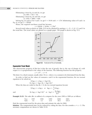
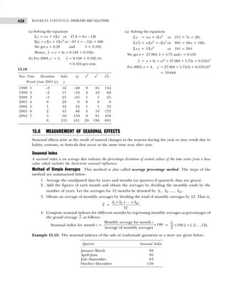
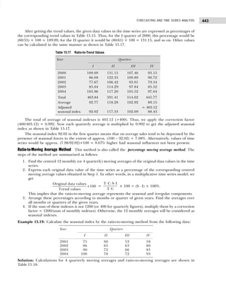
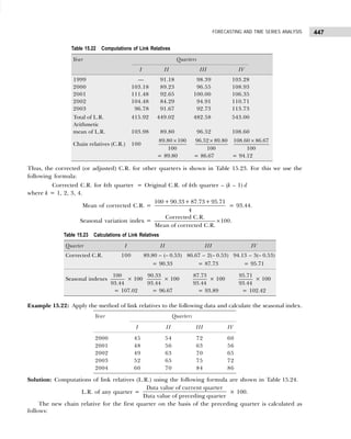
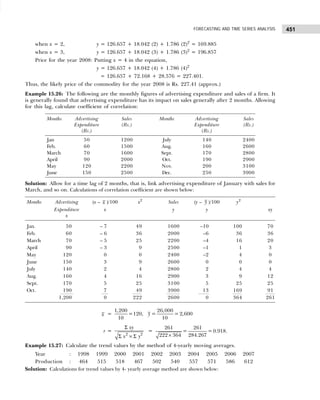
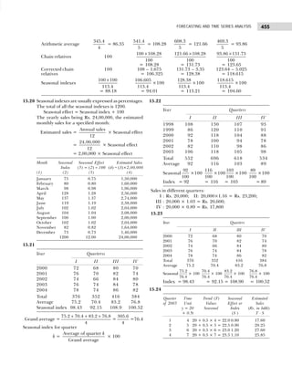
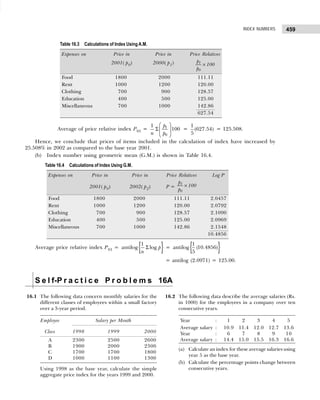
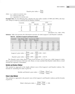
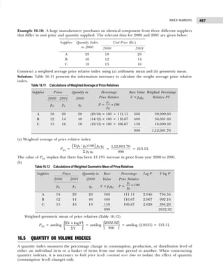
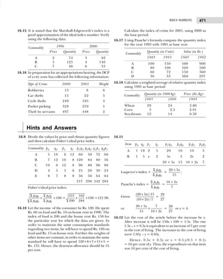
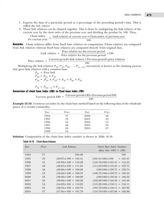
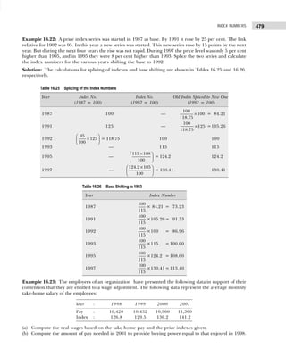
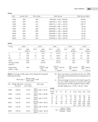
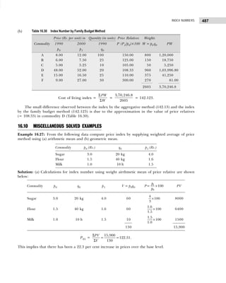
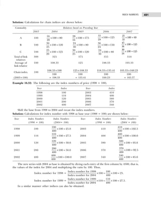
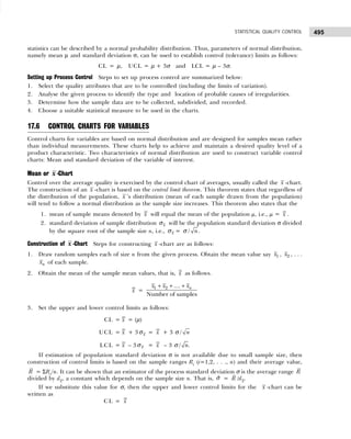
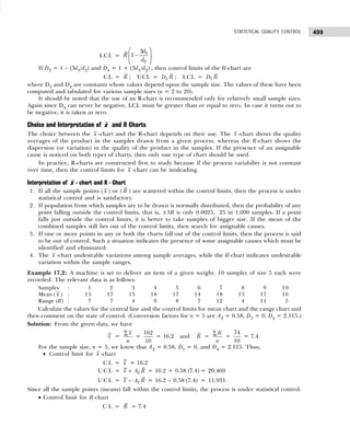
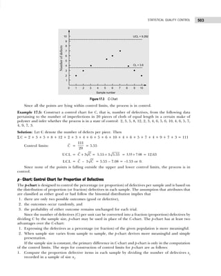
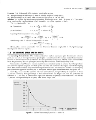
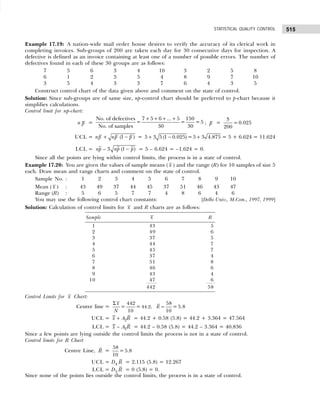
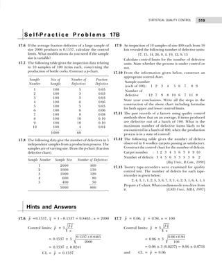
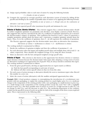
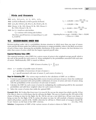
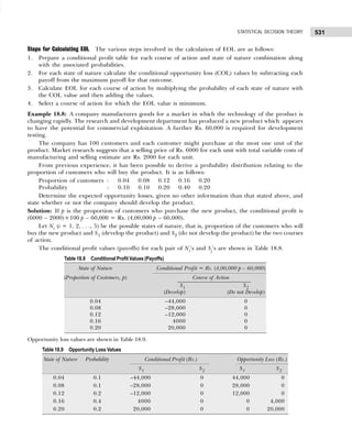
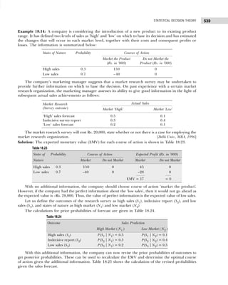
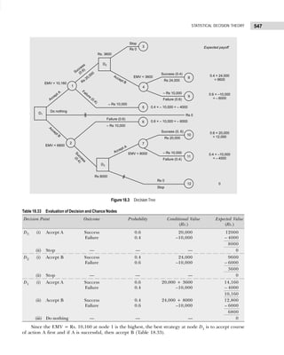
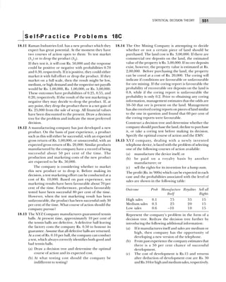
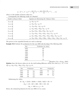
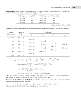
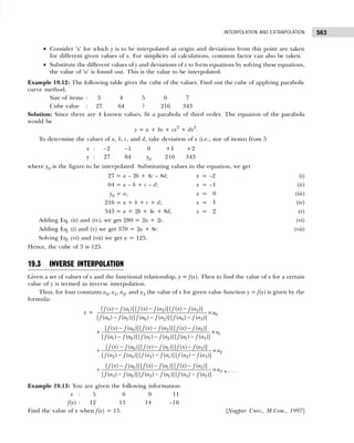
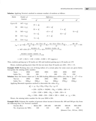
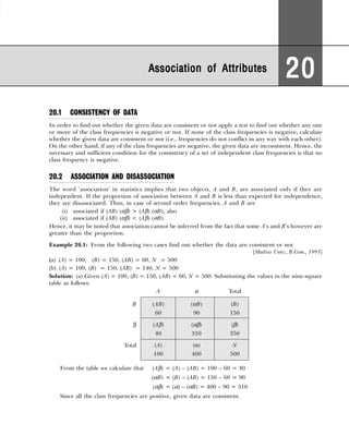
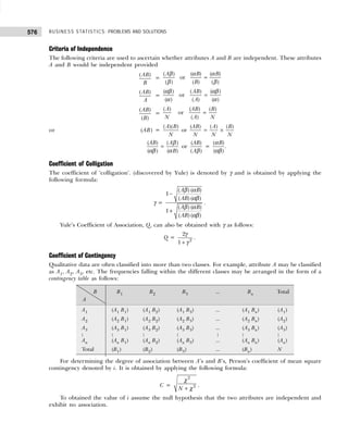
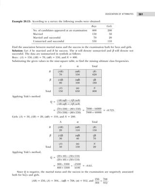
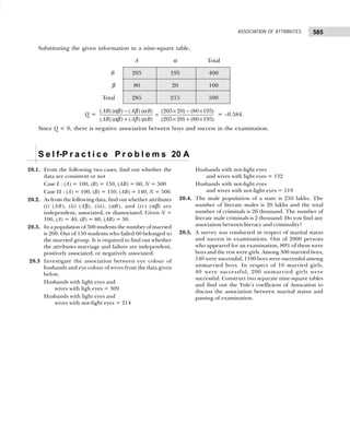
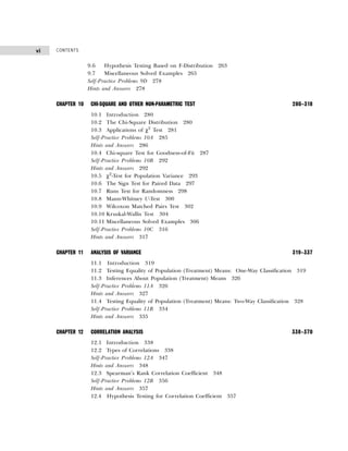
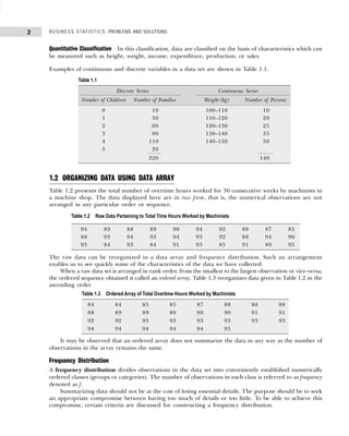
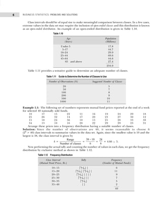
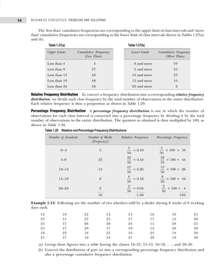
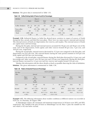
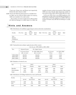
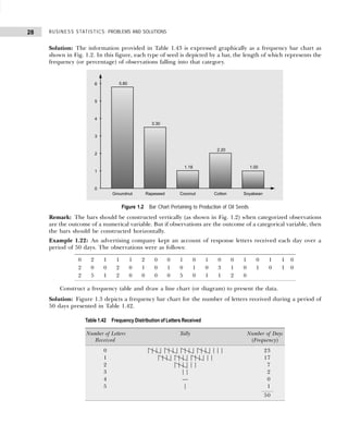
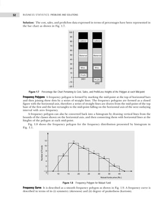
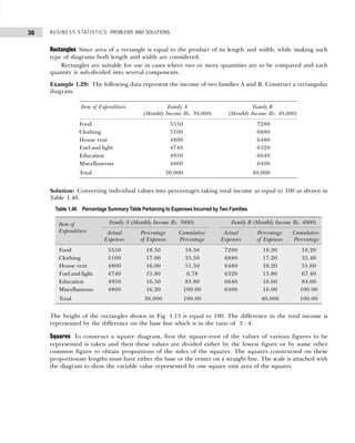
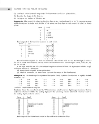
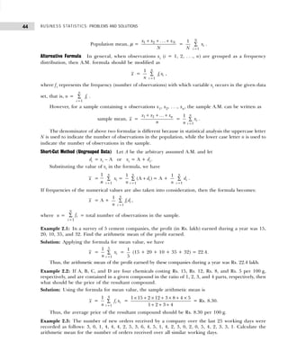
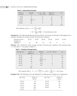
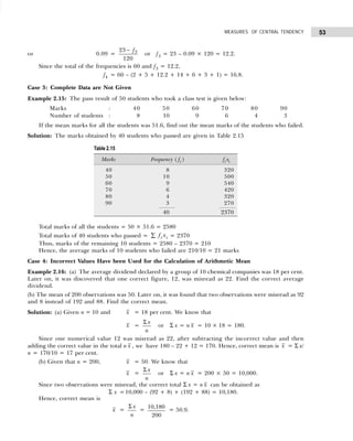
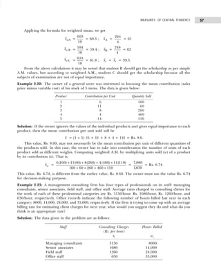
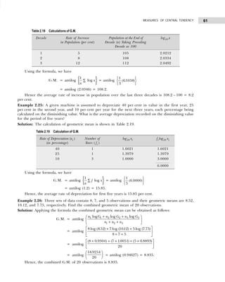
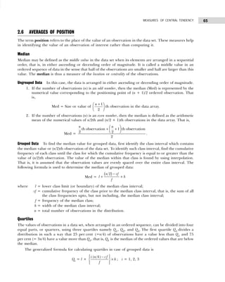
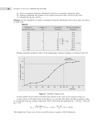
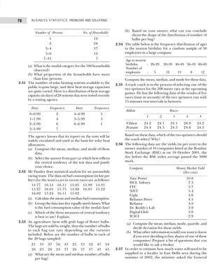
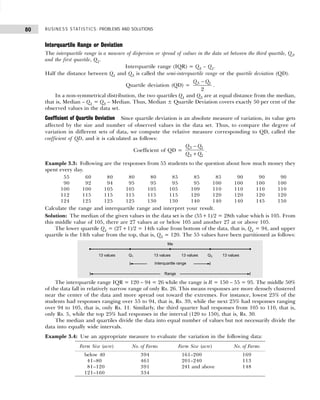
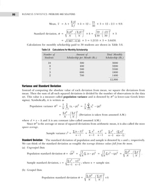
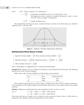
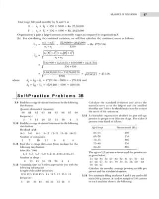
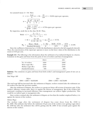
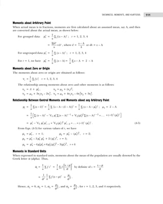
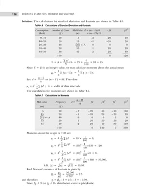
Example 1.7: Marks obtained by 50 students are given below:
31 13 46 31 30 45 38 42 30 9
30 30 46 36 2 41 44 18 29 63
44 30 19 5 44 15 7 25 12 30
6 22 24 37 15 6 39 32 21 20
42 31 19 14 23 28 17 53 22 21
Construct a grouped frequency distribution. [Calicut Univ., M.Com., 2006]
Solution: Since the number of observations are 50, we may choose 6(26
>50) or less classes.
The lowest value is 2 and largest 63, the class intervals shall be
h =
Range
Number of Classes
= ≈
63 – 2 61
= =10.1 11
6 6
.
The frequency distribution is shown in Table 1.19.
Table 1.19 Frequency Distribution
Marks Tallies Frequency
(Number of Students)
2–12 |||| || 7
13–23 |||| |||| |||| 14
24–34 |||| |||| |||| 14
35–45 |||| |||| |||| 13
45–56 | 1
57–67 1 1
50
Example 1.8: Point out the mistakes in the following table to show the distribution of population according
to sex, age, and literacy.
Sex 0–25 25–25 50–75 75–100
Males
Females
[Bombay Univ., M.Com., 1995]
Solution: All the characteristics are not revealed in the given table. The characteristic of literacy are
complete and hence table needs to be re-arranged as shown in Table 1.20.
Table 1.20 Distribution of Population According to Age, Sex, and Literacy
Age Groups Literates Illiterates Total
M F Total M F Total M F Total
0–25 — — — — — — — — —
25–50 — — — — — — — — —
50–75 — — — — — — — — —
75–100 — — — — — — — — —
Total — — — — — — — — —
Example 1.9: (a) Present the following data of the percentage marks of 60 students in the form of a
frequency table with 10 classes of equal width, one class being 50–59.
41 17 33 63 54 92 60 58 70 06 67 82
33 44 57 49 34 73 54 63 36 52 32 75
60 33 09 79 28 30 42 93 43 80 03 32
57 67 24 64 63 11 35 82 10 23 00 41
60 32 72 53 92 88 62 55 60 33 40 57
[CSI, Foundation, 2007]](https://image.slidesharecdn.com/businessstatisticsproblemsandsolutions-230910073954-6d42a210/85/Business-Statistics_-Problems-and-Solutions-pdf-24-320.jpg)
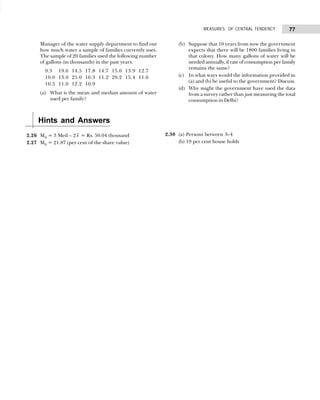
![11
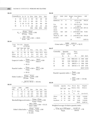
DATA CLASSIFICATION, TABULATION, AND PRESENTATION
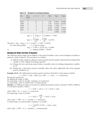
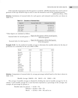
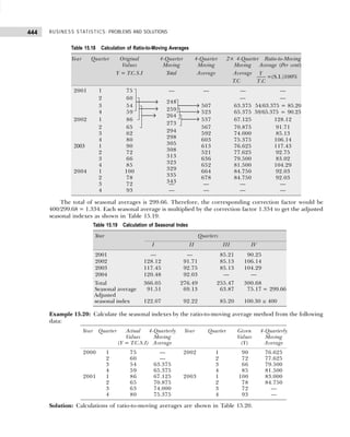
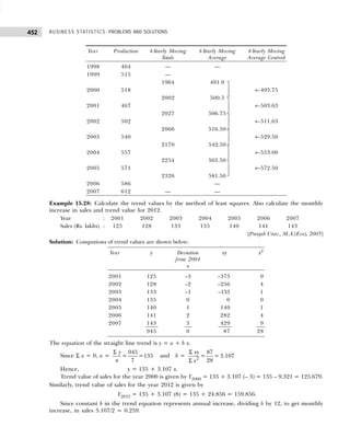
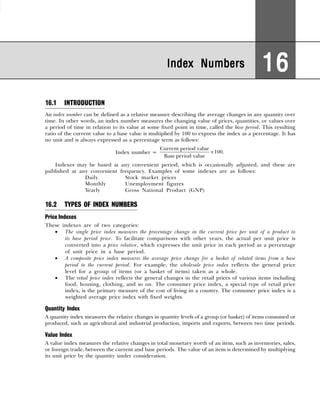
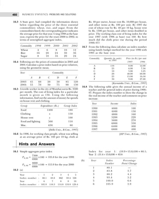
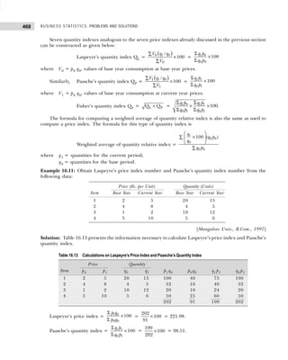
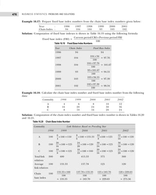
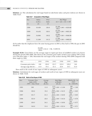
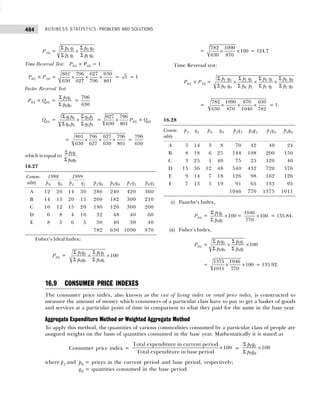
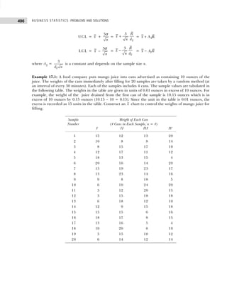
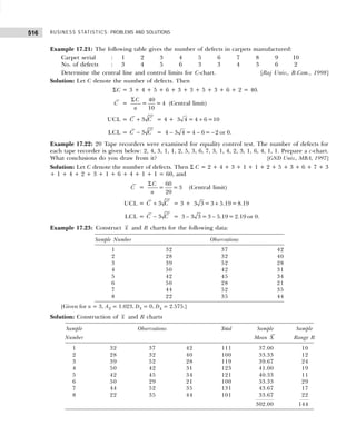
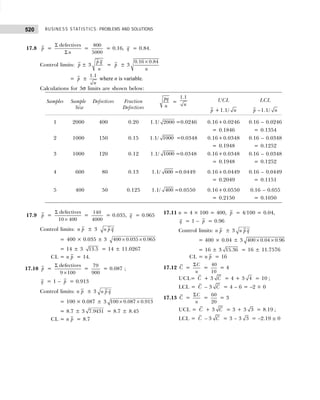
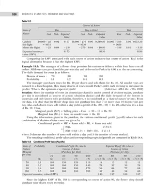
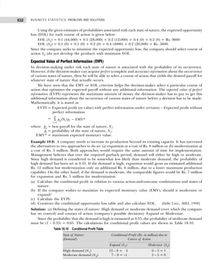
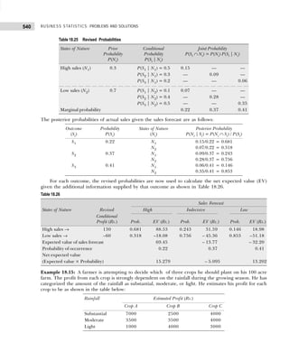
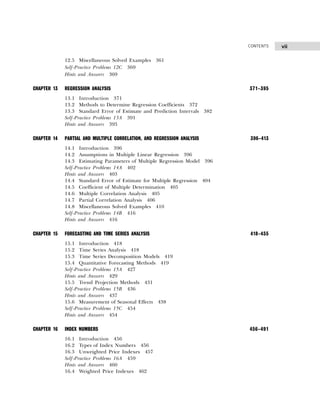
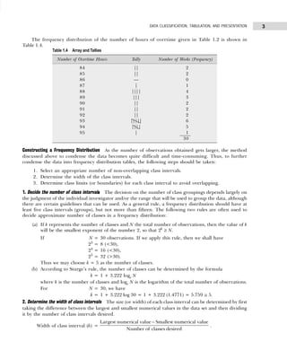
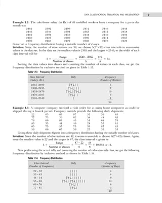
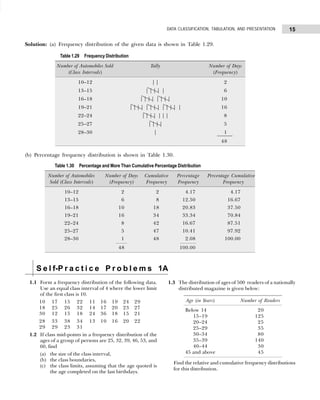
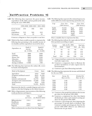
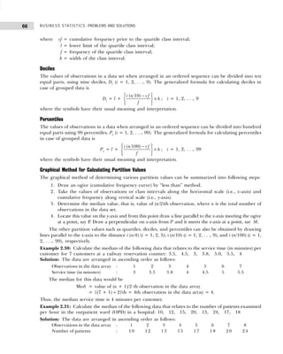
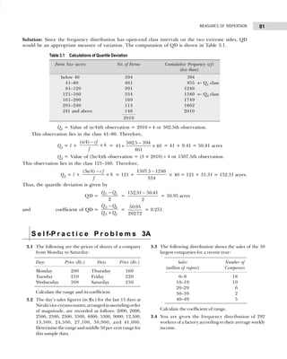
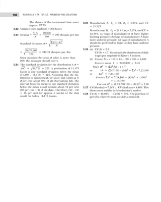
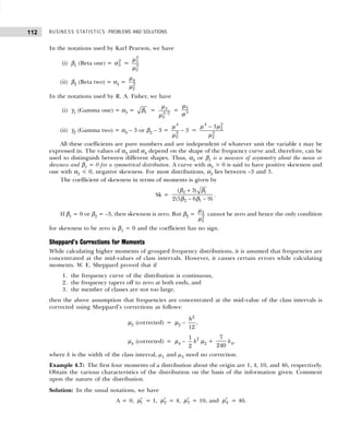
(b) A sample consists of 34 observations recorded correct to the nearest integer, ranging in value from
201 to 337. If it is decided to use seven classes of width 20 integers and to begin in the first class at 199.5,
find the class marks of the seven classes. [Calicut Univ., B.Sc., 2004]
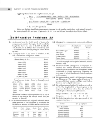
Solution: (a) Since the number of observations are 60, we may choose 6(26
> 60) or less class intervals.
The class interval is given by
h =
Range
Number of class
=
93 – 0
6
= 15 (approx.)
The frequency distribution with inclusive intervals is shown in Table 1.21.
Table 1.21 Frequency Distribution
Marks Tallies Frequency
0–15 ||||| 6
16–31 |||| 5
32–47 |||| |||| |||| | 16
48–63 |||| |||| |||| ||| 18
64–79 |||| ||| 8
80–95 |||| || 7
60
(b) Since it is decided to begin with 199.5 and takes a classes interval of 20, the first class will be
199.5–219.5, the second would be 219.5–239.5, and so on. The class mark shall be obtained by adding
the lower and upper limits and dividing it by 2. Thus, for the first class, the marks shall be (199.5) +
(219.5)/2 = 209.5. Since class interval is equal the other class marks can be obtained by adding 20 to
the preceding class mark. Table 1.22 gives the class limits and class marks of the seven classes.
Table 1.22
Class Limits Class Marks
199.5–219.5 206.5
219.5–239.5 229.5
239.5–259.5 249.5
259.5–279.5 269.5
279.5–299.5 289.5
299.5–319.5 309.5
319.5–339.5 329.5
Bivariate Frequency Distribution
The frequency distributions discussed so far involved only one variable and are therefore called univariate
frequency distributions. In case the data involve two variables (such as profit and expenditure on advertisements
of a group of companies, income and expenditure of a group of individuals, supply and demand of a
commodity, etc.), then frequency distribution so obtained as a result of cross classification is called bivariate
frequency distribution. It can be summarized in the form of a two-way (bivariate) frequency table and the values
of each variable are grouped into various classes (not necessarily same for each variable) in the same way
as for univariate distributions.
Frequency distribution of variable x for a given value of y is obtained by the values of x and vice versa.
Such frequencies in each cell are called conditional frequencies. The frequencies of the values of variables x
and y together with their frequency totals are called the marginal frequencies.
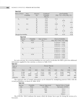
Example 1.10: The following figures indicate income (x) and percentage expenditure on food (y) of 25
families. Construct a bivariate frequency table classifying x into intervals 200–300, 300–400, . . ., and y
into 10–15, 15–20, . . .](https://image.slidesharecdn.com/businessstatisticsproblemsandsolutions-230910073954-6d42a210/85/Business-Statistics_-Problems-and-Solutions-pdf-25-320.jpg)
![13
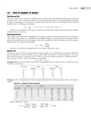
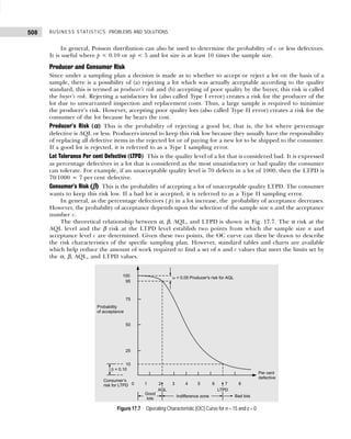
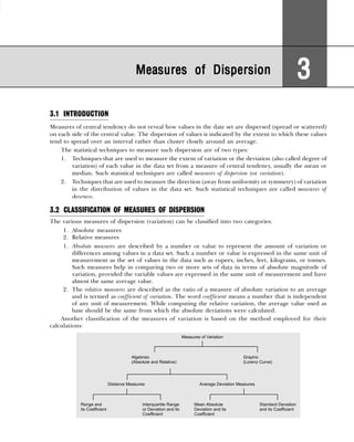
DATA CLASSIFICATION, TABULATION, AND PRESENTATION
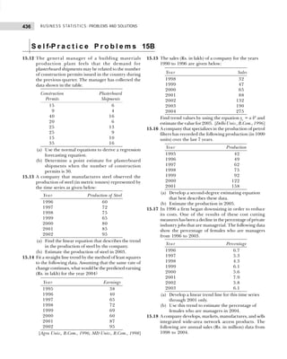
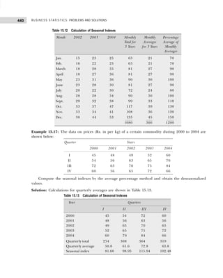
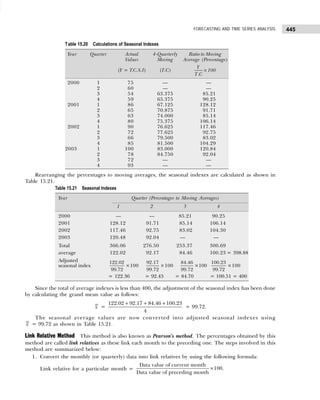
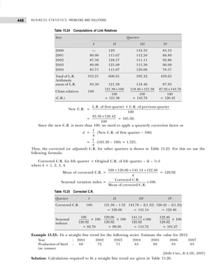
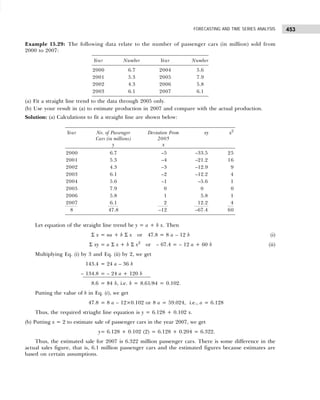
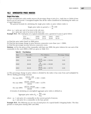
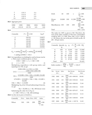
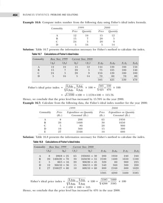
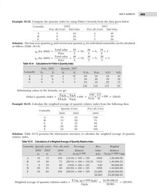
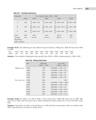
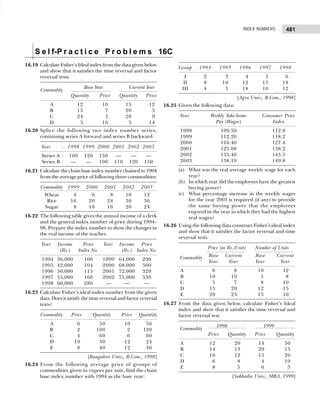
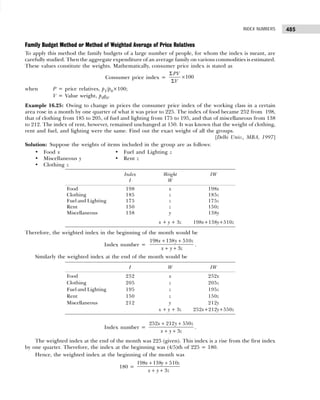
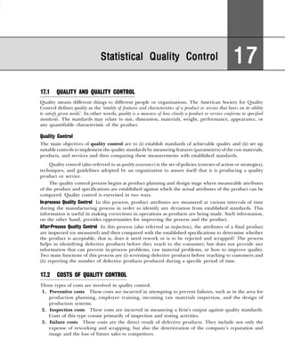
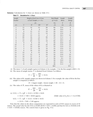
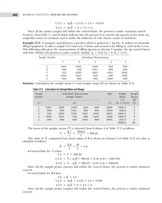
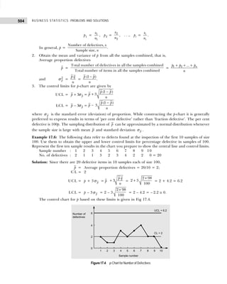
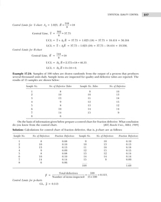
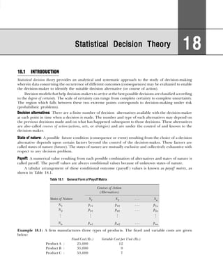
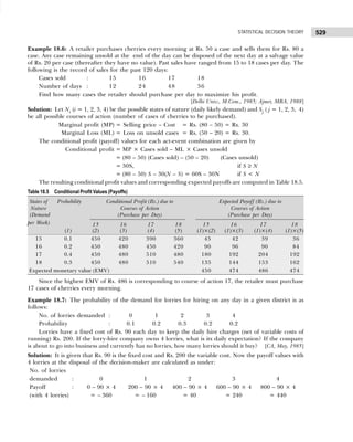
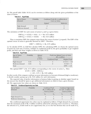
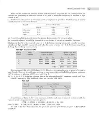
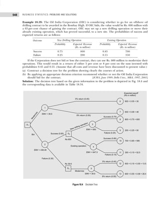
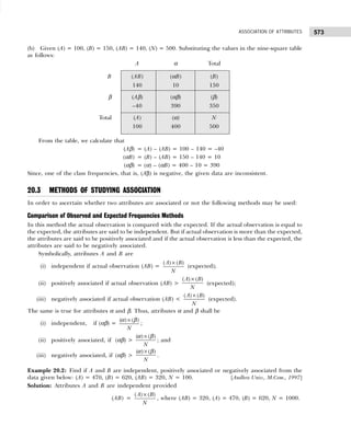
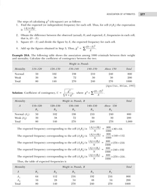
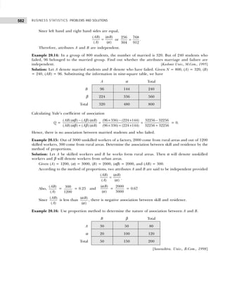
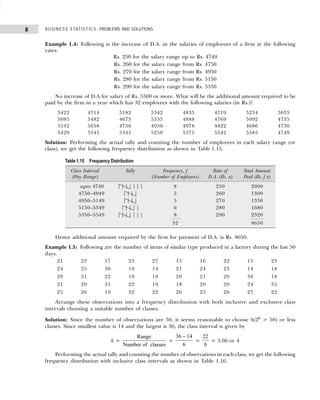
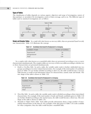
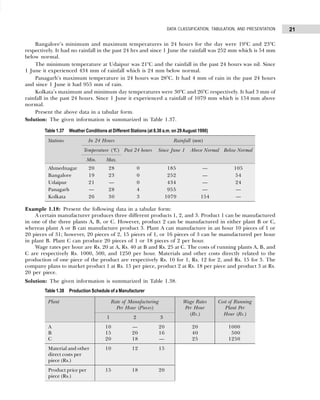
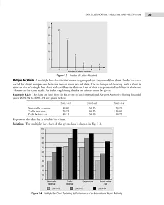
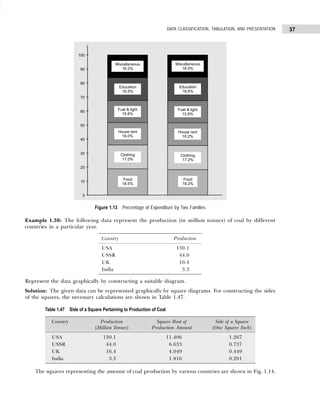
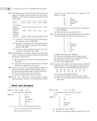
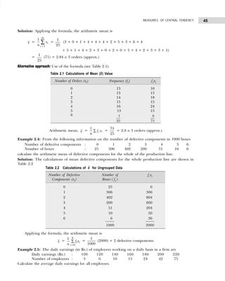
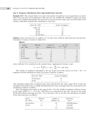
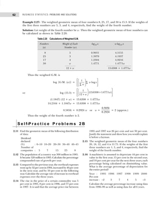
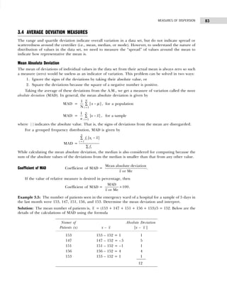
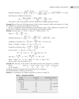
(ii) Conditional frequency distribution for Y given X>15.
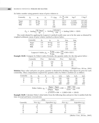
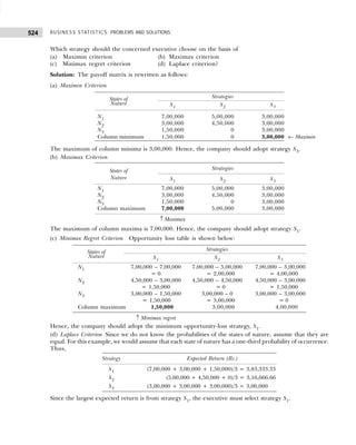
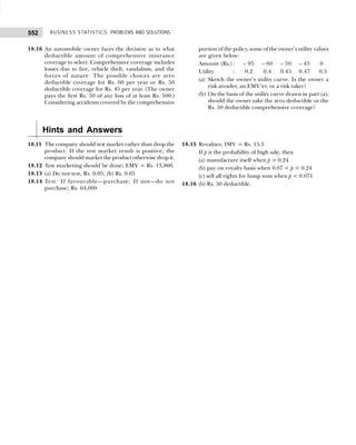
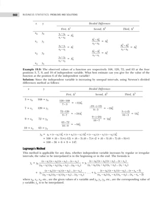
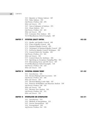
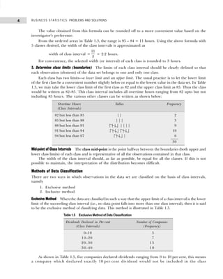
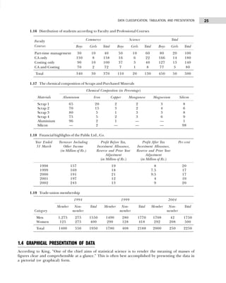
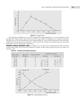
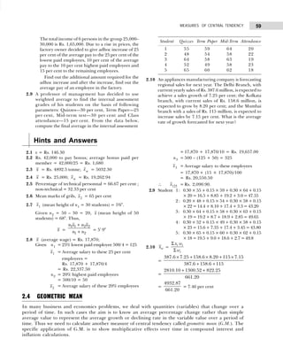
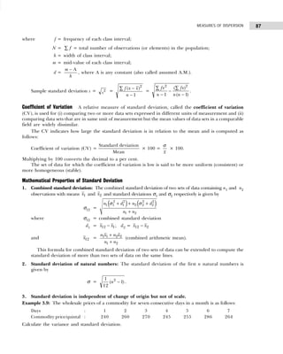
Example 1.12: 30 pairs of values of two variables X and Y are given below. From a two-way table,
X 14 20 33 25 41 18 24 29 38 45
Y 148 242 296 312 518 196 214 340 492 568
X 23 32 37 19 28 34 38 29 44 40
Y 282 400 288 292 431 440 500 512 415 514
X 22 39 43 44 12 27 39 38 17 26
Y 282 481 516 598 122 200 451 387 245 413
Take class intervals of X as 10–20, 20–30, etc., and that of Y as 100–200, 200–300. etc.
[Osmania Univ., B.Com., 2006]
Solution: The two-way frequency distribution is shown in Table 1.25.
Table 1.25 Bivariable Frequency Table
Y↓ X→ 10–20 20–30 30–40 40–50 Total
100–200 ||| (3) — — — 3
200–300 || (2) |||| (5) || (2) — 9
300–400 — || (2) | (1) — 3
400–500 — || (2) |||| (5) | (1) 8
500–600 — | (1) | (1) |||| (5) 7
Total 5 10 9 6 30
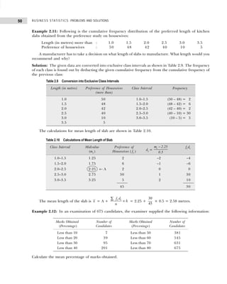
Types of Frequency Distributions
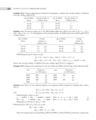
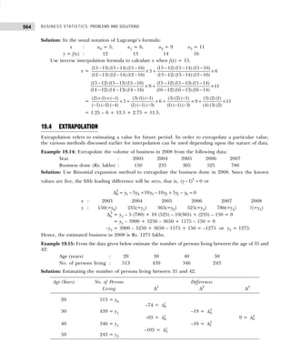
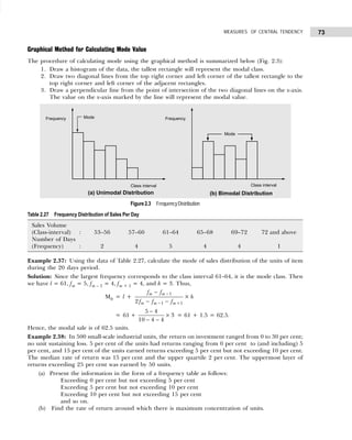
Cumulative Frequency Distribution Sometimes it is preferable to present data in a cumulative frequency (cf )
distribution. A cumulative frequency distribution is of two types: (i) more than type and (ii) less than type.
In a less than cumulative frequency distribution, the frequencies of each class interval are added
successively from top to bottom and represent the cumulative number of observations less than or equal
to the class frequency to which it relates. But in the more than cumulative frequency distribution, the
frequencies of each class interval are added successively from bottom to top and represent the cumulative
number of observations greater than or equal to the class frequency to which it relates.
The frequency distribution given in Table 1.26 illustrates the concept of cumulative frequency
distribution.
Player Y Player X
15–19 20–24
5–9 1 —
10–14 1 —
15–19 3 1
20–24 1 1
6 2
Table 1.26 Cumulative Frequency Distribution
Number of Accidents Number of Weeks Cumulative Frequency Cumulative Frequency
(Frequency) (less than) (more than)
0–4 5 5 45 + 5 = 50
5–9 22 5 + 22 = 27 23 + 22 = 45
10–14 13 27 + 13 = 40 10 + 13 = 23
15–19 8 40 + 8 = 48 2 + 8 = 10
20–24 2 48 + 2 = 50 2](https://image.slidesharecdn.com/businessstatisticsproblemsandsolutions-230910073954-6d42a210/85/Business-Statistics_-Problems-and-Solutions-pdf-27-320.jpg)
![BUSINESS STATISTICS: PROBLEMS AND SOLUTIONS
16
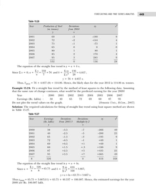
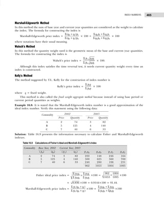
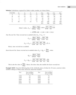
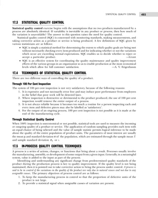
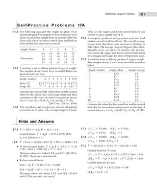
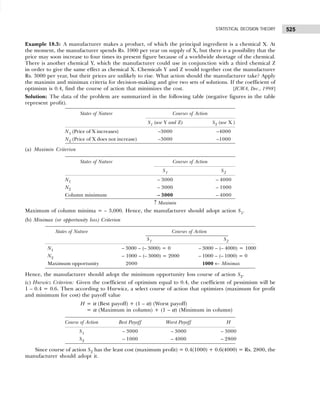
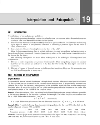
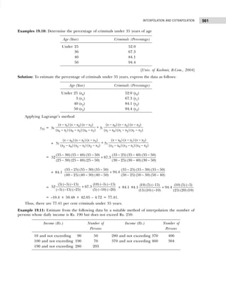
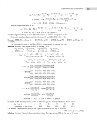
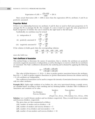
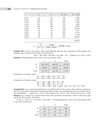
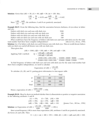
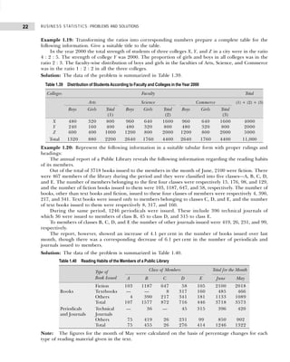
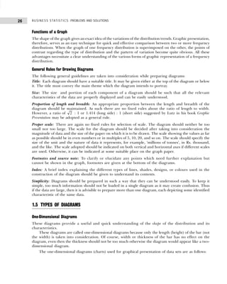
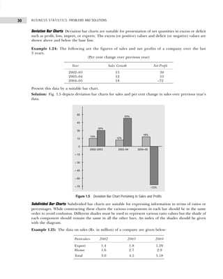
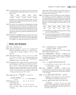
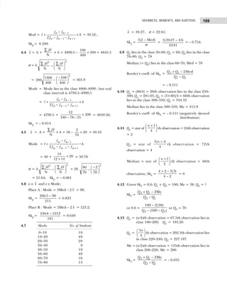
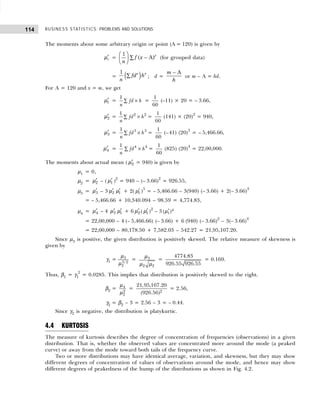
1.4 The distribution of inventory to sales ratio of 200 retail
outlets is given below:
Inventory to Sales Ratio Number of Retail Outlets
1.0–1.2 20
1.2–1.4 30
1.4–1.6 60
1.6–1.8 40
1.8–2.0 30
2.0–2.2 15
2.2–2.4 5
Find the relative and cumulative frequency
distributions for this distribution.
1.5 A wholesaler’s daily shipments of a particular item
varied from 1,152 to 9,888 units per day. Indicate the
limits of nine classes into which these shipments might
be grouped.
1.6 A college book store groups the monetary value of its
sales into a frequency distribution with the classes,
Rs. 400–500, Rs. 501–600, and Rs. 601 and over. Is it
possible to determine from this distribution the
amount of sales
(a) less than Rs. 601 (b) less than Rs. 501
(c) Rs. 501 or more?
1.7 Theclassmarksofdistributionofthenumberofelectric
lightbulbsreplaceddailyinanofficebuildingare5,10,
15, and 20. Find (a) the class boundaries and (b) class
limits.
1.8 The marks obtained by 25 students in Statistics and
Economics are given below. The first figure in the
bracket indicates the marks in Statistics and the second
in Economics.
(14, 12) (0, 2) (1, 5) (7, 3) (15, 9)
(2, 8) (12, 18) (9, 11) (5, 3) (17, 13)
(19, 18) (11, 7) (10, 13) (13, 16) (16, 14)
(6, 10) (4, 1) (9, 15) (11, 14) (8, 3)
(13, 11) (14, 17) (10, 10) (11, 7) (15, 15)
Prepare a two-way frequency table taking the width of
each class interval as 4 marks, the first being less than 4.
1.9 Prepare a bivariate frequency distribution for the
following data for 20 students:
Marks in Law: 10 11 10 11 11
14 12 12 13 10
Marks in Statistics: 20 21 22 21 23
23 22 21 24 23
Marks in Law: 13 12 11 12 10
14 14 12 13 10
Marks in Statistics: 24 23 22 23 22
22 24 20 24 23
Also prepare
(a) a marginal frequency table for marks in Law and
Statistics
(b) a conditional frequency distribution for marks in
Law when the marks in Statistics are more than 22.
1.10 Classify the following data by taking class intervals
such that their mid-values are 17, 22, 27, 32, and so
on:
30 42 30 54 40 48 15 17 51
42 25 41 30 27 42 36 28 26
37 54 44 31 36 40 36 22 30
31 19 48 16 42 32 21 22 46
33 41 21
[Madurai-Kamraj Univ., B.Com., 1995]
1.11 In degree colleges of a city, no teacher is less than 30
years or more than 60 years in age. Their cumulative
frequencies are as follows:
Less than : 60 55 50 45
40 35 30 25
Total frequency : 980 925 810 675
535 380 220 75
Find the frequencies in the class intervals 25–30,
30–35, . . .
H i n t s a n d A n s w e r s
1.1 The classes for preparing frequency distribution by
inclusive method will be
10–13, 14–17, 18–21, . . ., 34–37, 38–41
1.2 (a) Size of the class interval = Difference between the
mid-values of any two consecutive classes = 7
(b) The class boundaries for different classes are
obtained by adding (for upper class boundaries
or limits) and subtracting (for lower class
boundaries or limits) half the magnitude of the
class interval, that is, 7 ÷ 2 = 3.5 from the mid-
values.
Class Intervals:
21.5–28.5 28.5–35.5 35.5–42.5
Mid-Values: 25 32 39
Class Intervals:
42.5–49.5 49.5–56.5 56.5–63.5
Mid-Values: 46 53 60
(c) The distribution can be expressed in inclusive
class intervals with width of 7 as 22–28, 29–35,
. . ., 56–63.
1.5 One possibility is 1000–1999, 2000–2999,
3000–3999, . . ., 9000–9999 units of the item.](https://image.slidesharecdn.com/businessstatisticsproblemsandsolutions-230910073954-6d42a210/85/Business-Statistics_-Problems-and-Solutions-pdf-30-320.jpg)
![17
DATA CLASSIFICATION, TABULATION, AND PRESENTATION
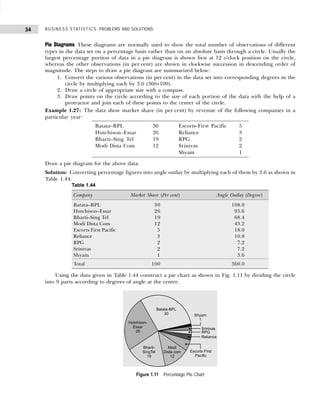
1.11
Age (year) Cumulative
Frequency Age Frequency
Less than 25 275 20–25 75
Less than 30 220 25–30 220 – 75 = 145
Less than 35 380 30–35 380 – 220 = 160
Less than 40 535 35–40 535 – 380 = 155
1.3 TABULATION OF DATA
Tabulation is another way of summarizing and presenting the given data in a systematic form in rows and
columns. Such presentation facilitates comparisons by bringing related information close to each other
and helps in further statistical analysis and interpretation.
Parts of a Table
1. Table number: A table should be numbered for easy identification and reference in future. The table
number may be given either in the centre or side of the table but above the top of the title of the table.
If the number of columns in a table is large, then these can also be numbered so that easy reference to
these is possible.
2. Title of the table: Each table must have a brief, self-explanatory, and complete title which can
(a) indicate the nature of data contained.
(b) explain the locality (i.e., geographical or physical) of data covered.
(c) indicate the time (or period) of data obtained.
(d) contain the source of the data to indicate the authority for the data, as a means of verification and as
a reference. The source is always placed below the table.
3. Caption and stubs: The headings for columns and rows are called caption and stub, respectively.
They must be clear and concise.
4. Body: The body of the table should contain the numerical information. The numerical information is
arranged according to the descriptions given for each column and row.
5. Prefactory or head note: If needed, a prefactory note is given just below the title for its further
description in a prominent type. It is usually enclosed in brackets and is about the unit of measurement.
6. Footnotes: Anything written below the table is called a footnote. It is written to further clarify either
the title captions or stubs. For example, if the data described in the table pertain to profits earned by
a company, then the footnote may define whether it is profit before tax or after tax. There are various
ways of identifying footnotes:
(a) Numbering footnotes consecutively with small number 1, 2, 3, ..., or letters a, b, c, ..., or star *,
**, . . .
(b) Sometimes symbols like @ or $ are also used to identify footnotes.
A blank model table is given below:
Age (year) Cumulative
Frequency Age Frequency
Less than 45 675 40–45 675 – 535 = 140
Less than 50 810 45–50 810 – 675 = 135
Less than 55 925 50–55 925 – 810 = 115
Less than 60 980 55–60 980 – 925 = 55
Table Number and Title [Head or Prefactory Note (if any)]
Stub Heading Caption Total (Rows)
Subhead Subhead
Column-head Column-head Column-head Column-head
Stub Entries
Total (Columns)
Footnote :
Source Note :](https://image.slidesharecdn.com/businessstatisticsproblemsandsolutions-230910073954-6d42a210/85/Business-Statistics_-Problems-and-Solutions-pdf-31-320.jpg)
![49
MEASURES OF CENTRAL TENDENCY
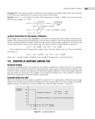
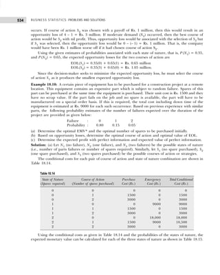
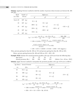
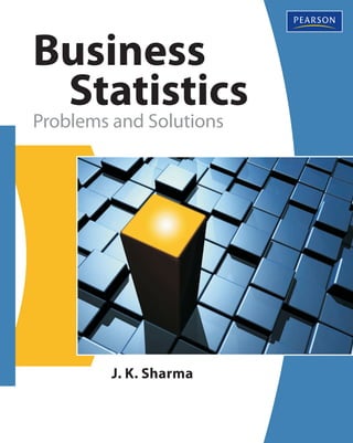
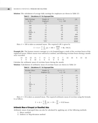
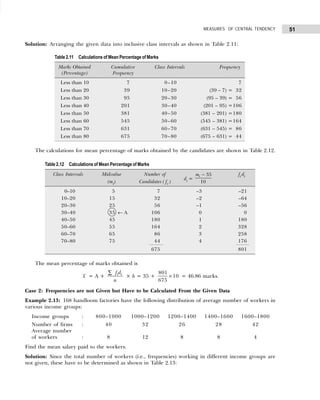
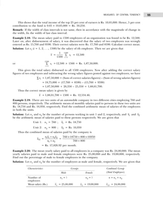
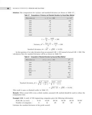
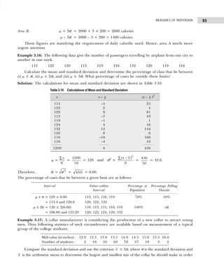
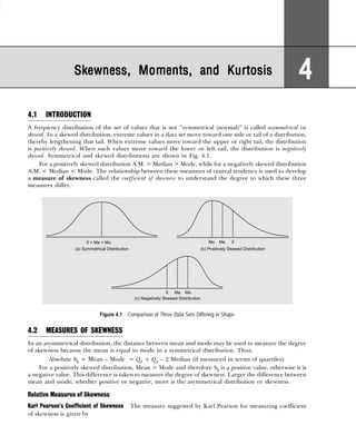
Due to continuous losses, it is desired to bring down the manpower strength to 30 per cent of the
present number according to the following scheme:
(a) Retrench the first 15 per cent from the lower age group.
(b) Absorb the next 45 per cent in other branches.
(c) Make 10 per cent from the highest age group retire permanently, if necessary.
Calculate the age limits of the persons retained and those to be transferred to other departments. Also
find the average age of those retained. [Delhi Univ., MBA, 2003]
Solution: (a) The first 15 per cent persons to be retrenched from the lower age groups are (15/100)×1000
= 150. But the lowest age group 20–25 has only 30 persons and therefore the remaining 150 – 30 = 120
will be taken from next higher age group, that is, 25–30, which has 160 persons.
(b) The next 45 per cent, that is, (45/100)×1000 = 450 persons who are to be absorbed in other
branches, belong to the following age groups:
(c) Those who are likely to be retired are 10 per cent, that is, (10/100) × 1000 = 100 persons and
belong to the following highest age groups:
Hence, the calculations of the average age of those retained and/or to be transferred to other departments
are shown in Table 2.8.
The required average age is x = A +
d f
n
h
i i
∑
× = 47.5 –
55
5
300
× = 46.58 = 47 years (approx.).
Some Special Types of Problems and Their Solutions
Case 1: Frequencies are Given in Cumulative Form, that is, Either “More Than Type” or “Less Than
Type”
That the “more than type” cumulative frequencies are calculated by adding frequencies from bottom to
top, so that the first class interval has the highest cumulative frequency and it goes on decreasing in
subsequent classes. But in case of “less than cumulative frequencies,” the cumulation is done downward
so that the first class interval has the lowest cumulative frequency and it goes on increasing in the subsequent
classes.
Age Groups Number of Persons
25–30 (160 – 120) = 40
30–35 210
35–40 180
40–45 (450 – 40 – 210 – 180) = 20
Age Group Number of Persons
55–60 (100 – 40) = 60
60–65 40
Table 2.8 Calculations of Average Age
Age Group Midvalue, Number of di = (xi – 47.5)/5 fi di
(xi) ( mi ) Persons ( fi )
40–45 42.5 145 – 20 = 125 –1 –125
45–50 47.5 ← A 105 0 0
50–55 52.5 70 1 70
300 –55](https://image.slidesharecdn.com/businessstatisticsproblemsandsolutions-230910073954-6d42a210/85/Business-Statistics_-Problems-and-Solutions-pdf-63-320.jpg)
![BUSINESS STATISTICS: PROBLEMS AND SOLUTIONS
68
Median observation = (n/2)th = (3000) ÷ 2 = 1500th observation. This observation lies in the class
interval 201–250.
Now applying the formula, we have
Med = l +
( )
n cf
f
h
2 −
×
= 201 +
1500 730
900
50
−
× = 201 + 42.77 = Rs. 243.77.
Hence, the median wage is Rs. 243.77 per day.
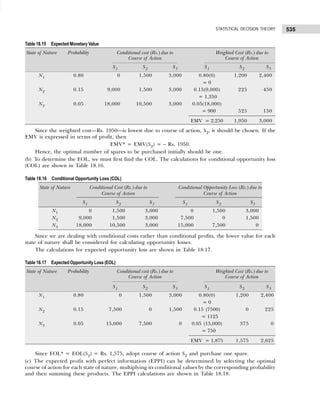
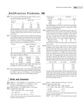
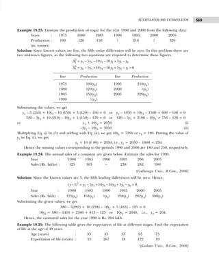
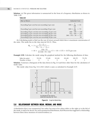
Example 2.34: The following is the distribution of weekly wages of 600 workers in a factory:
(a) Draw an ogive for the above data and hence obtain the median value. Check it against the calculated
value.
(b) Obtain the limits of weekly wages of central 50 per cent of the workers.
(c) Estimate graphically the percentage of workers who earned weekly wages between 950 and 1250.
[Delhi Univ., MBA, 1996]
Solution: (a) The calculations of median value are shown in Table 2.24.
Since a median observation in the data set is the (n/2)th observation = (600 ÷ 2)th observation, that is,
300th observation. This observation lies in the class interval 950–1025. Applying the formula to calculate
median wage value, we have
Med = l +
( / )
n cf
f
h
2 −
×
= 950 +
300 236
207
75
−
× = 950 + 23.2 = Rs. 973.2 per week.
The median wage value can also be obtained by applying the graphical method as shown in Fig. 2.1.
Weekly Wages Number of Weekly Wages Number of
(in Rs.) Workers (in Rs.) Workers
Below 875 69 1100–1175 58
875–950 167 1175–1250 24
950–1025 207 1250–1325 10
1025–1100 65 600
Table 2.24 Calculations of Median Value
Weekly Wages Number of Cumulative Frequency Percent Cumulative
(in Rs.) Workers ( f ) (Less than type) Frequency
Less than 875 69 69 11.50
Less than 950 167 236 ← Q1 class 39.33
Less than 1025 207 443 ← Median class 73.83
Less than 1100 65 508 ← Q3 class 84.66
Less than 1175 58 566 94.33
Less than 1250 24 590 98.33
Less than 1325 10 600 100.00](https://image.slidesharecdn.com/businessstatisticsproblemsandsolutions-230910073954-6d42a210/85/Business-Statistics_-Problems-and-Solutions-pdf-82-320.jpg)
![71
MEASURES OF CENTRAL TENDENCY
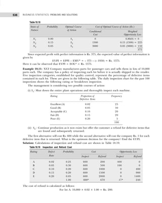
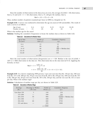
Example 2.36: The following distribution gives the pattern of overtime work per week done by 100
employees of a company. Calculate median, first quartile, and seventh decile.
Overtime hours : 10–15 15–20 20–25 25–30 30–35 35–40
No. of employees : 11 20 35 20 8 6
[Kurukshetra Univ., MBA, 1997]
Calculate Q1, D7, and P60.
Solution: The calculations of median, first quartile (Q1), and seventh decile (D7) are shown in Table 2.26.
Since the number of observations in this data set are 100, the median value is (n/2)th = (100 ÷ 2)th
= 50th observation. This observation lies in the class interval 20–25. Applying the formula to get median
overtime hours value, we have
Med = l +
( / )
n cf
f
h
2 −
×
= 20 +
50 31
35
5
−
× = 20 + 2.714 = 22.714 hours.
Q1 = value of (n/4) th observation = value of (100/4)th = 25th observation.
Thus, Q1 = l +
( / )
n cf
f
h
4 −
× = 15 +
25 11
20
5
−
× = 15 + 3.5 = 18.5 hours
D7 = value of (7n/10)th observation = value of (7 × 100)/10 = 70th observation.
Thus, D7 = l +
( / )
7 10
n cf
f
h
−
× = 25 +
70 66
20
5
−
× = 25 + 1 = 26 hours
P60 = Value of (60n/100) th observation = 60×(100/100) = 60th observation.
Thus, P60 = l +
(60 /100)
n cf
f
× −
× h = 20 +
60 31
35
−
× 5 = 24.14 hours.
Table 2.26
Overtime Hours Number of Cumulative Frequency
Employees (Less than type)
10–15 11 11
15–20 20 31 ← Q1 class
20–25 35 66 ← Median and P60 class
25–30 20 86 ← D7 class
30–35 8 94
35–40 6 100
100
S e l f-P r a c t i c e P r o b l e m s 2 C
2.21 The following are the profit figures earned by 50
companies in the country
Profit (in Rs. lakh) Number of Companies
10 or less 14
20 or less 10
30 or less 30
40 or less 40
50 or less 47
60 or less 50
Calculate
(a) the median
(b) the range of profit earned by the middle 80
per cent of the companies. Also verify your results
by graphical method.
2.22 A number of particular items have been classified
according to their weights. After drying for two weeks
the same items have again been weighted and similarly
classified. It is known that the median weight in the](https://image.slidesharecdn.com/businessstatisticsproblemsandsolutions-230910073954-6d42a210/85/Business-Statistics_-Problems-and-Solutions-pdf-85-320.jpg)
![BUSINESS STATISTICS: PROBLEMS AND SOLUTIONS
72
first weighing was 20.83 g, while in the second
weighing it was 17.35 g. Some frequencies, a and b, in
the first weighing and x and y in the second weighing
are missing. It is known that a = x/3 and b = y/2. Find
out the values of the missing frequencies.
Class Frequencies Class Frequencies
I II I II
0–5 a x 15–20 52 50
5–10 b y 20–25 75 30
10–15 11 40 25–30 22 28
2.23 The length of time taken by each of 18 workers to
complete a specific job was observed to be the
following:
Time (in min) : 5–9 10–14 15–19 20–24 25–29
Number of workers : 3 8 4 2 1
(a) Calculate the median time
(b) Calculate Q1 and Q3
2.24 The following distribution is with regard to weight (in
g) of mangoes of a given variety. If mangoes less than
443 g in weight be considered unsuitable for the
foreign market, what is the percentage of total yield
suitable for it? Assume the given frequency
distribution to be typical of the variety.
Weight Number of Weight Number of
(in g) Mangoes (in g) Mangoes
410–419 10 450–459 45
420–429 20 460–469 18
430–439 42 470–479 17
440–449 54
Draw an ogive of “more than” type of the above data
and deduce how many mangoes will be more than
443 g.
2.25 Gupta Machine Company has a contract with its
customers to supply machined pump gears. One
requirement is that the diameter of gears be within
specific limits. Here are the diameters (in inches) of a
sample of 20 gears:
4.01 4.00 4.02 4.02 4.03 4.00
3.98 3.99 3.99 4.01 3.99 3.98
3.97 4.00 4.02 4.01 4.02 4.00
4.01 3.99
What can Gupta say to his customers about the
diameters of 95 per cent of the gears they are receiving?
[Delhi Univ., MBA, 1998]
Hints and Answers
2.21 Med = 27.5; P90 – P10 = 47.14 – 11.67 = 35.47
2.22 a = 3, b = 6; x = 9, y = 12
2.23 (a) 13.25 (b) Q3 = 17.6, Q1 = 10.4
2.24 52.25%; 103
2.25 Diameter
size : 3.973.98 3.994.00 4.014.02 4.03
Frequency : 1 2 4 4 4 4 1
x =
x
n
∑
=
80.04
20
= 4.002 inches;
s =
Σ (x x
n
−
−
)2
1
=
2 2
1
{ ( ) }
1
x n x
n
−
∑
−
=
2
1
{(320.32 20 (4.002) }
19
−
= 0.016 inches 95% of the gears will have diameter
in the interval : x ± 2s = (4.002 ± 0.016)
2.7 MODE
The mode is that value of an observation which occurs most frequently in the data set, that is, the point (or
class mark) with the highest frequency.
In the case of grouped data, the following formula is used for calculating mode:
Mode =
1
1 1
2
m m
m m m
f f
l h
f f f
−
− +
−
+ ×
− −
where l = lower limit of the model class interval;
fm – 1 = frequency of the class preceding the mode class interval;
fm+1 = frequency of the class following the mode class interval;
h = width of the mode class interval.](https://image.slidesharecdn.com/businessstatisticsproblemsandsolutions-230910073954-6d42a210/85/Business-Statistics_-Problems-and-Solutions-pdf-86-320.jpg)
![BUSINESS STATISTICS: PROBLEMS AND SOLUTIONS
82
Weekly Income No. of Weekly Income No. of
(Rs.) Workers (Rs.) Workers
Below 1350 08 1450–1470 22
1350–1370 16 1470–1490 15
1370–1390 39 1490–1510 15
1390–1410 58 1510–1530 9
1410–1430 60 1530 and above 10
1430–1450 40
Calculate the quartile deviation and its coefficient from
the above mentioned data.
[Kurukshetra Univ., MBA, 1998]
3.5 You are given the data pertaining to kilowatt hours of
electricity consumed by 100 persons in a city.
Consumption No. of Users
(kilowatt hour)
10–10 06
10–20 25
20–30 36
30–40 20
40–50 13
Calculate the range within which the middle
50 per cent of the consumers fall.
3.6 The following sample shows the weekly number of
road accidents in a city during a two-year period:
Number of Frequency Number of Frequency
Accidents Accidents
1 0–4 05 25–29 9
1 5–9 12 30–34 4
10–14 32 35–39 3
15–19 27 40–44 1
20–24 11
Find the interquartile range and coefficient of quartile
deviation.
3.7 A City Development Authority subdivided the available
land for housing into the following building lot sizes:
Lot Size Frequency
(square meters)
Below 69.44 19
69.44–104.15 25
104.16–208.32 42
208.33–312.49 12
312.50–416.65 5
416.66 and above 17
Find the interquartile range and quartile deviation.
3.8 The cholera cases reported in different hospitals of a
city in a rainy season are given below:
Calculate the quartile deviation for the given
distribution and comment upon the meaning of your
result.
Age Group Frequency Age Group Frequency
(years) (years)
Less than 1 15 25–35 132
1–5 113 35–45 65
5–10 122 45–65 46
10–15 91 65 and above 15
15–25 229
Hints and Answers
3.1 Range = Rs. 90; coefficient of range = 0.219
3.2 Range = Rs. 39,000;
Middle 50%, R = P75 – P25
= x(75n/100) + (1/2)–x(25n/100) + (1/2)
= x(11.25 + 0.50) – x(3.75 + 0.50)
= x11.75 – x4.25
= (13,500 + 8250) – (2500 + 00)
= 19,250
Here x11.75 is the interpolated value for the 75% of the
distance between 11th and 12th ordered sales amount.
Similarly, x4.25 is the interpolated value for the 25% of
the distance between 4th and 5th order sales amount.
3.3 Coefficient of range = 1
3.4 Quartile deviation = 27.76; Coeff. of QD = 0.020;
Q1 = 1393.48; Q3 = 1449
3.5 Q3 – Q1 = 34 – 17.6 = 16.4
3.6 Q3 – Q1 = 30.06; coefficient of QD = 0.561
3.7 Q3 – Q1 = 540.26; QD = 270.13
3.8 QD = 10 years](https://image.slidesharecdn.com/businessstatisticsproblemsandsolutions-230910073954-6d42a210/85/Business-Statistics_-Problems-and-Solutions-pdf-96-320.jpg)
![85
MEASURES OF DISPERSION
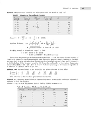
Thus, the average sales is Rs. 179.91 thousand per day and the mean absolute deviation of sales is
Rs. 47.01 thousand per day.
Example 3.8: A welfare organization introduced an education scholarship scheme for school going
children of a backward village. The rates of scholarship were fixed as given below:
The ages of 30 school children are noted as 11, 8, 10, 5, 7, 12, 7, 17, 5, 13, 9, 8, 10, 15, 7, 12, 6, 7,
8, 11, 14, 18, 6, 13, 9, 10, 6, 15, 3, 5 years, respectively. Calculate mean and standard deviation of monthly
scholarship. Find out the total monthly scholarship amount being paid to the students. [IGNOU, MBA, 2002]
Solution: The number of students in the age group from 5–7 to 17–19 are calculated as shown in Table 3.4:
The calculations for mean and standard deviation are shown in Table 3.5.
Table 3.3 Calculations for MAD
Sales Mid-value Frequency (m – 175)/50 fd |x – x | f |x – x |
(Rs.) (m) ( f ) (= d ) = |x – x |
50–100 75 11 –2 –22 104.91 1154.01
100–150 125 23 –1 –23 54.91 1262.93
150–200 175 ← A 44 0 0 4.91 216.04
200–250 225 19 1 19 45.09 856.71
250–300 275 8 2 16 95.09 760.72
300–350 325 7 3 21 145.09 1015.63
112 11 5266.04
Age Group (years) Amount of Scholarship
per Month (Rs.)
5–7 300
8–10 400
11–13 500
14–16 600
17–19 700
Table 3.4
Age Group (years) Tally Bars Number of Students
5–7 | | | | | | | | 10
8–10 | | | | | | | 8
11–13 | | | | | | 7
14–16 | | | 3
17–19 | | 2
30
Table 3.5 Calculations for Mean and Standard Deviation
Age Group Number of Mid-value d =
−
m A
h
fd fd2
(years) Students (f) (m)
5–7 10 6 –2 –20 40
08–10 8 9 –1 –8 8
11–13 7 A → 12 0 0 0
14–16 3 15 1 3 3
17–19 2 18 2 4 8
30 –21 59
=
− 12
3
m](https://image.slidesharecdn.com/businessstatisticsproblemsandsolutions-230910073954-6d42a210/85/Business-Statistics_-Problems-and-Solutions-pdf-99-320.jpg)
![BUSINESS STATISTICS: PROBLEMS AND SOLUTIONS
90
Standard deviation for proposal A:
sA =
f x x
f
( )
−
∑
∑
2
= 87,21,404.4 = Rs. 2953.20.
Standard deviation for proposal B:
sB =
f x x
f
( )
−
∑
∑
2
= 14 08 37 579
, , , = Rs. 11,867.50.
The sA < sB indicates uniform net profit for proposal A. Thus, proposal A may be chosen.
Example 3.12: For a group of 50 male workers, the mean and standard deviation of their monthly wages
are Rs. 6300 and Rs. 900 respectively. For a group of 40 female workers, these are Rs. 5400 and Rs. 600
respectively. Find the standard deviation of monthly wages for the combined group of workers.
[Delhi Univ., MBA, 2002]
Solution: Given that n1 = 50, x1 = 6300, σ1 = 900
n2 = 40, x2 = 5400, σ2 = 600
Then, combined mean x12 =
n x n x
n n
1 1 2 2
1 2
+
+
=
50 6300 40 5400
50 40
× + ×
+
= 5,900
and combined standard deviation
σ12 =
( ) ( )
2 2 2 2
1 1 1 2 2 2
1 2
n d n d
n n
σ σ
+ + +
+
=
50(8,10,000 1,60,000) 40(3,60,000 2,50,000)
50 40
+ + +
+
= Rs. 900
where d1 = x x
12 1
− = 5900 – 6300 = – 400;
d2 = x x
12 2
− = 5900 – 5400 = 500.
Example 3.13: A study of the age of 100 persons grouped into intervals 20–22, 22–24, 24–26,..., revealed
the mean age and standard deviation to be 32.02 and 13.18 respectively. While checking it was discovered
that the observation 57 was misread as 27. Calculate the correct mean age and standard deviation.
[Delhi Univ., MBA, 1997]
Solution: From the data given in the problem, we have x = 32.02, σ = 13.18, and N = 100.
We know that
NPV(xi) Expected NPV ( x ) x – x f f (x – x )2
1559 5485 –3926 0.30 46,24,042.8
5662 5485 177 0.40 12,531.6
9175 5485 3690 0.30 40,84,830.0
1.00 87,21,404.4
NPV (xi ) Expected NPV ( x ) x – x f f (x – x )2
–10,050 5485 –15,535 0.30 7,24,00,867.5
5812 5485 327 0.40 42,771.6
20,584 5485 15,099 0.30 6,83,93,940
1.00 14,08,37,579](https://image.slidesharecdn.com/businessstatisticsproblemsandsolutions-230910073954-6d42a210/85/Business-Statistics_-Problems-and-Solutions-pdf-104-320.jpg)
![91
MEASURES OF DISPERSION
x =
N
f x
∑
or Σ f x = N× x = 100× 32.02 = 3202
and σ 2
=
2
2
( )
f x
x
N
∑
− or Σ fx2
= N[σ 2
+ ( x )2
] = 100[(13.18)2
+ (32.02)2
]
= 100(173.71 + 1025.28) = 100×1198.99 = 1,19,899.
On replacing the correct observation, we get
Σ fx = 3202 – 27 + 57 = 3232.
Also, Σ fx2
= 1,19,899 – (27)2
+ (57)2
= 1,19,899 – 729 + 3248 = 1,22,419.
Thus, correct A.M. is
x =
fx
N
∑
=
3232
100
= 32.32.
and correct variance is
σ 2
=
2
2
( )
fx
x
N
∑
− =
1,22,419
100
– (32.32)2
= 1224.19 – 1044.58 = 179.61
or correct standard deviation
σ = 2
σ = 179.61 = 13.402.
Example 3.14: The mean of 5 observations is 15 and the variance is 9. If two more observations having
values – 3 and 10 are combined with these 5 observations, what will be the new mean and variance of 7
observations.
Solution: From the data of the problem, we have x = 15, s2
= 9, and n = 5. We know that
x =
x
n
∑
or x
∑ = n × x = 5 × 15 = 75.
If two more observations having values –3 and 10 are added to the existing 5 observations, then after
adding these 6th and 7th observations, we get
x
∑ =75 – 3 + 10 = 82.
Thus, the new A.M. is x =
x
n
∑
=
82
7
= 11.71
Variance s2
=
x
n
x
2
2
∑
− ( )
9 =
x
n
2
2
15
∑
− ( ) or x2
∑ = 1170.
On adding two more observations, that is, –3 and 10, we get
x2
∑ =1170 + (– 3)2
+ (10)2
= 1279
Variance s2
=
x
n
x
2
2
∑
− ( ) =
1279
7
– (11.71)2
= 45.59.
Hence, the new mean and variance of 7 observations is 11.71 and 45.59, respectively.
Chebyshev’s Theorem
For any set of data (population or sample) and any constant z greater than 1 (but need not be an integer), the proportion of the
values that lie within z standard deviations on either side of the mean is at least {1 – (1/z2
)}. That is,
RF (|x – µ| ≤ z σ) ≥ 1 –
1
2
z](https://image.slidesharecdn.com/businessstatisticsproblemsandsolutions-230910073954-6d42a210/85/Business-Statistics_-Problems-and-Solutions-pdf-105-320.jpg)
![BUSINESS STATISTICS: PROBLEMS AND SOLUTIONS
94
to meet the needs of practically all the customers bearing in mind that collar are worn on average half
inch longer than neck size.
Solution: Calculations for mean and standard deviation in order to determine the range of collar size to
meet the needs of customers are shown in Table 3.11.
Mean, x = A +
fd
h
N
∑
× = 14.0 –
98
250
× 0.5 = 14.0 – 0.195 = 13.805.
Standard deviation, σ =
2
2
fd fd
N N
∑ ∑
−
× h =
2
548 98
250 250
−
−
× 0.5
= 2.192 – 0.153 × 0.5 = 1.427 × 0.5 = 0.7135.
Largest and smallest neck size = x ± 3σ = 13.805 ± 3 × 0.173
= 11.666 and 15.944.
Since all the customers are to wear collar half inch longer than their neck size, 0.5 is to be added to
the neck size range given above. The new range then becomes
(11.666 + 0.5) and (15.944 + 0.5) or 12.165 and 16.444, that is, 12.2 and 16.4 inches.
Example 3.18: The breaking strength of 80 “test pieces” of a certain alloy is given in the following table,
the unit being given to the nearest thousand grams per square inch:
Calculate the average breaking strength of the alloy and the standard deviation. Calculate the percentage
of observations lying between x ± 2σ. [Vikram Univ., MBA, 2000]
Table 3.11 Calculations for Mean and Standard Deviation
Mid-value Number of
14
0.5
x A x
h
− −
= fd fd2
(in inches) Students
12.0 2 –4 –8 32
12.5 16 –3 –48 144
13.0 36 –2 –72 144
13.5 60 –1 –60 60
14.0 ← A 76 0 0 0
14.5 37 1 37 37
15.0 18 2 36 72
15.5 3 3 9 27
16.0 2 4 8 32
N = 250 –98 548
Breaking Strength Number of Pieces
44–46 3
46–48 24
48–50 27
50–52 21
52–54 5](https://image.slidesharecdn.com/businessstatisticsproblemsandsolutions-230910073954-6d42a210/85/Business-Statistics_-Problems-and-Solutions-pdf-108-320.jpg)
![BUSINESS STATISTICS: PROBLEMS AND SOLUTIONS
98
Tea Contents Machine A Machine B
(g)
485–490 12 10
490–495 18 15
495–500 20 24
500–505 22 20
505–510 24 18
510–515 04 13
Comment on the performance of the two machines
on the basis of average filling and dispersion.
3.15 An analysis of production rejects resulted in the
following observations
No. of Rejects No. of No. of Rejects No. of
per Operator Operators per Operator Operators
21–25 05 41–45 15
26–30 15 46–50 12
31–35 28 51–55 03
36–40 42
Calculate the mean and standard deviation.
[Delhi Univ., MBA, 2000]
3.16 Blood serum cholestrerol levels of 10 persons are as
under:
240 260 290 245 255 288 272 263 277 250
Calculate the standard deviation with the help of
assumed mean
3.17 32 trials of a process to finish a certain job revealed the
following information:
Mean time taken to complete the job = 80 minutes
Standard deviation = 16 minutes
Another set of 8 trials gave mean time as 100 minutes
and standard deviation equalled to 25 minutes.
Find the combined mean and standard deviation.
3.18 From the analysis of monthly wages paid to workers
in two organizations X and Y, the following results
were obtained:
X Y
Number of wage-earners : 0550 600.
Average monthly wages (Rs.): 1260 1348.5
Variance of distribution of
wages (Rs.) : 0100 841.
Obtain the average wages and the variability in
individual wages of all the workers in the two
organizations taken together.
3.19 An analysis of the results of a budget survey of 150
families showed an average monthly expenditure of
Rs. 120 on food items with a standard deviation of
Rs. 15. After the analysis was completed it was noted
that the figure recorded for one household was wrongly
taken as Rs. 15 instead of Rs. 105. Determine the
correct value of the average expenditure and its
standard deviation.
3.20 The standard deviation of a distribution of 100 values
was Rs. 2. If the sum of the squares of the actual
values was Rs. 3,600, what was the mean of this
distribution?
3.21 An air-charter company has been requested to quote
a realistic turn-round time for a contract to handle
certain imports and exports of a fragile nature.
The contract manager has provided the
management accountant with the following analysis
of turn-round times for similar goods over a given
period of 12 months.
Turn-round Time Frequency
(hours)
Less than 2 25
2 and < 14 36
4 and < 16 66
6 and < 18 47
8 and < 10 26
10 and < 12 18
12 and < 14 02
(a) Calculate mean and standard deviation.
(b) Advise the contract manager about the turn-round
time to be quoted using
(i) mean plus one standard deviation;
(ii) mean plus two standard deviations.
3.22 The hourly output of a new machine is four times that
of the old machine. If the variance of the hourly output
of the old machine in a period of n hours is 16, what is
the variance of the hourly output of the new machine
in the same period of n hours.
3.23 The number of cheques cashed each day at the five
branches of a bank during the past month has the
following frequency distribution:
Number of Cheques Frequency
200–199 10
200–399 13
400–599 17
600–799 42
800–999 18
The General Manager, Operations, for the bank,
knows that a standard deviation in cheque cashing
of more than 200 checks per day creates staffing
problem at the branches because of the uneven
workload. Should the manager worry about staff-
ing next month?
3.24 Mr. Gupta, owner of a bakery, said that the average
weekly production level of his company was 11,398](https://image.slidesharecdn.com/businessstatisticsproblemsandsolutions-230910073954-6d42a210/85/Business-Statistics_-Problems-and-Solutions-pdf-112-320.jpg)
![99
MEASURES OF DISPERSION
loaves and the variance was 49,729. If data used to
compute the results were collected for 32 weeks,
during how many weeks was the production level
below 11,175 and above 11,844?
3.25 Suppose that samples of polythene bags from two
manufacturers A and B are tested by a buyer for
bursting pressure, giving the following results:
Bursting Number of Bags
Pressure A B
5.0–9.9 2 09
10.0–14.9 9 11
15.0–19.9 29 18
20.0–24.9 54 32
25.0–29.9 11 27
30.0–34.9 5 13
(a) Which set of bags has the highest bursting
pressure?
(b) Which has more uniform pressure? If prices are
the same, which manufacturer’s bags would be
preferred by the buyer? Why?
[Delhi Univ., MBA, 1997]
3.26 The number of employees, average daily wages per
employee, and the variance of daily wages per
employee for two factories are given below:
Factory A Factory B
Number of employees : 050 100
Average daily wages (Rs.) : 120 085
Variance of daily wages (Rs.) : 009 016
(a) In which factory is there greater variation in the
distribution of daily wages per employee?
(b) Suppose in Factory B the wages of an employee
were wrongly noted as Rs. 120 instead of
Rs. 100. What would be the correct variance for
Factory B?
3.27 The share prices of a company in Mumbai and Kolkata
markets during the last 10 months are recorded
below:
Month Mumbai Kolkata
January 105 108
February 120 117
March 115 120
April 118 130
May 130 100
June 127 125
July 109 125
August 110 120
September 104 110
October 112 135
Determine the arithmetic mean and standard deviation
of prices of shares. In which market are the share
prices more stable? [HP Univ., MBA, 2002]
3.28 A person owns two petrol filling stations A and B. At
station A, a representative sample of 200 consumers
who purchase petrol was taken. The results were as
follows:
Number of Litres of Number of
Petrol Purchased Consumers
00 0and < 2 15
02 0and < 4 40
04 0and < 6 65
06 0and < 8 40
008 and < 10 30
10 and over 10
A similar sample at station B users showed a mean of
4 litres with a standard deviation of 2.2 litres. At which
station is the purchase of petrol relatively more
variable?
Hints and Answers
3.9 MAD = 1.239; x = 63.89
3.10 x = 10.68; MAD = 3.823
3.11 Med = 6.612; MAD = 2.252
3.12 x = 13.013 inches; σ = 0.8706 inches; x + 3σ =
14.884 (largest size); x – 3σ = 13.142 (smallest size)
3.13 x = Rs. 280.2; σ = Rs. 60.765
3.14 Machine A: x1 = 499.5; σ1 = 7.14; Machine B :
x2 = 500.5; σ2 = 7.40
3.15 x = 36.96; σ = 6.375
3.16 σ = 16.48
3.17 x12 = 84 minutes; σ12 = 19.84
3.18 x12 = Rs. 1306; σ12 = Rs. 53.14
3.19 Corrected x = Rs. 120.6 and corrected σ = Rs. 12.4
3.20 x = 5.66
3.21 (a) (i) x = 5.68 ; (ii) σ = 2.88
(b) (i) x + σ = 5.68 + 2.88 = 8.56 hours
The chance of this turn-round time cover
approx. 84%
(ii) x + 2σ = 5.68 + 2 (2.88) = 11.44 hours](https://image.slidesharecdn.com/businessstatisticsproblemsandsolutions-230910073954-6d42a210/85/Business-Statistics_-Problems-and-Solutions-pdf-113-320.jpg)
![BUSINESS STATISTICS: PROBLEMS AND SOLUTIONS
104
Uniformity in the Wage Structure
The extent of relative uniformity in the wage structure before and after the settlement can be determined
by comparing the coefficient of variation as follows:
Before After
Coefficient of variation (CV)
300
2200
100
× = 13.63
260
2300
100
× = 11.30
Since CV has decreased after the settlement from 13.63 to 11.30, the distribution of wages is more
uniform after the settlement, that is, there is now comparatively less disparity in the wages received by the
workers. Such a position is good for both the workers and the management in maintaining a cordial work
environment.
Pattern of the Wage Structure
The nature and pattern of the wage structure before and after the settlement can be determined by
comparing the coefficients of skewness.
Before After
Coefficient of skewness (Skp)
3 2200 2500
300
( )
−
= – 3 3 2300 2400
260
( )
− = – 1.15
Since coefficient of skewness is negative and has increased after the settlement, it suggests that number
of workers getting low wages has increased and that of workers getting high wages has decreased after the
settlement.
Example 4.3: From the following data on age of employees, calculate the coefficient of skewness and
comment on the result
Age below (years) : 25 30 35 40 45 50 55
Number of employees : 8 20 40 65 80 92 100
[Delhi Univ., MBA, 1997]
Solution: The data are given in a cumulative frequency distribution form. So to calculate the coefficient
of skewness, convert this data into a simple frequency distribution as shown in Table 4.2.
Mean, x = A +
fd
N
∑
× h = 37.5 –
5
100
5
× = 37.25.
Mode value lies in the class interval 35–40. Thus,
Mo = l +
f f
f f f
h
m m
m m m
−
− −
×
−
− +
1
1 1
2
= 35 +
25 20
2 25 20 15
5
−
× − −
× = 35 +
5
15
5
× = 36.67.
Table 4.2 Calculations for Coefficient of Skewness
Age Mid-value Number of d = (m – A)/h f d f d2
( years) (m) Employees ( f ) = (m – 37.5)
20–25 22.5 8 –3 –24 72
25–30 27.5 12 –2 –24 48
30–35 32.5 20 ← fm – 1 –1 –20 20
35–40 37.5 25 ← fm 0 0 0
40–45 42.5 1 ← fm + 1 1 15 15
45–50 47.5 12 2 24 48
50–55 52.5 8 3 24 72
N = 100 –5 275](https://image.slidesharecdn.com/businessstatisticsproblemsandsolutions-230910073954-6d42a210/85/Business-Statistics_-Problems-and-Solutions-pdf-118-320.jpg)
![BUSINESS STATISTICS: PROBLEMS AND SOLUTIONS
106
Q1 = size of (N/4)th observation = (60 ÷ 4)th = 15th observation. Thus, Q1 lies in the class 10–20,
and
Q1 = l +
( /4)
N cf
h
f
−
×
= 10 +
15 5
12
10
−
R
S
T
U
V
W× = 10 + 8.33 = 18.33 lakh
Q3 = size of (3N/4)th observation = 45th observation. Thus, Q3 lies in the class 30–40, and
Q3 = l +
(3 /4)
N cf
h
f
−
×
= 30 +
45 37
16
10
−
R
S
T
U
V
W× = 30 + 5 = 35 lakh
Hence, the profit of central 50 per cent companies lies between Rs. 35 lakhs and Rs. 10.83 lakh.
Coefficient of quartile deviation, QD =
Q Q
Q Q
3 1
3 1
−
+
=
35 18 33
35 18 33
−
+
.
.
= 0.313.
(b) Median = size of (N/2)th observation = 30th observation. Thus, median lies in the class 20–30,
and
Median = l +
( /2)
N cf
h
f
−
×
= 20 +
30 17
20
10
−
R
S
T
U
V
W× = 20 + 6.5 = 26.5 lakh
Coefficient of skewness, Skb = 3 1
3 1
2Med
Q Q
Q Q
+ −
−
=
35 18 33 2 26 5
18 33
+ −
−
. ( . )
.
35
= 0.02.
The positive value of Skb indicates that the distribution is positively skewed, and therefore, there is a
concentration of larger values on the right side of the distribution.
Example 4.6: Apply an appropriate measure of skewness to describe the following frequency distribution.
[Bharthidasan Univ., MBA, 2001]
Solution: Since given frequency distribution is an open-ended distribution, Bowley’s method of calculating
skewness should be more appropriate. Calculations are shown in Table 4.4.
Q1 = size of (N/4)th observation = (420/4) = 105th observation. Thus, Q1 lies in the class 30–35 and
Age Number of Age Number of
(years) Employees (years) Employees
Below 20 13 35–40 112
20–25 29 40–45 94
25–30 46 45–50 45
30–35 60 50 and above 21
Table 4.4 Calculations for Bowley’s Coefficient of Skewness
Age (years) Number of Employees (f) Cumulative Frequency (cf)
Below 20 13 13
20–25 29 42
25–30 46 88
30–35 60 148 ← Q1 class
35–40 112 260
40–45 94 354 ← Q3 class
45–50 45 399
50 and above 21 420
N = 420](https://image.slidesharecdn.com/businessstatisticsproblemsandsolutions-230910073954-6d42a210/85/Business-Statistics_-Problems-and-Solutions-pdf-120-320.jpg)
![107
SKEWNESS, MOMENTS, AND KURTOSIS
Q1 = l +
( /4)
N cf
f
−
× h = 30 +
105 88
60
−
× 5 = 30 + 1.42 = 31.42 years
Q3 = size of (3N/4)th observation = (3 × 420/4) = 315th observation. Thus, Q3 lies in the class
40–45, and
Q3 = l +
(3 /4)
N cf
h
f
−
× = 40 +
315 260
5
94
−
× = 40 + 2.93 = 42.93 years
Median = size of (N/2)th = (420/2) = 210th observation. Thus, median lies in the class 35–40 and
Median =
( /2)
N cf
l h
f
−
+ × = 35 +
210 148
5
112
−
× = 35 + 2.77 = 37.77 years
Coefficient of skewness, Skb = 3 1
3 1
2Med
Q Q
Q Q
+ −
−
=
42.93 31.42 2 37.77
42.93 31.42
+ − ×
−
= –
1.19
11.51
= –0.103.
The negative value of Skb indicates that the distribution is negatively skewed.
S e l f-P r a c t i c e P r o b l e m s 4A
4.1 The following data relate to the profits (in Rs. ’000) of
1,000 companies:
Profits : 100–120 120–140 140–160 160–180
180–200 200–220 220–240
No. of 17 53 199 194
companies : 327 208 2
Calculate the coefficient of skewness and comment on
its value. [MD Univ., MBA, 2001]
4.2 A survey was conducted by a manufacturing company
to find out the maximum price at which people would
be willing to buy its product. The following table gives
the stated price (in rupees) by 100 persons:
Price : 2.80–2.90 2.90–3.00 3.00–3.10
3.10–3.20 3.20–3.30
No. of 11 29 18
persons: 27 15
Calculate the coefficient of skewness and interpret its
value.
4.3 Calculate coefficient of variation and Karl Pearson’s
coefficient of skewness from the data given below:
Marks (less than) : 20 40 60 80 100
No. of students : 18 40 70 90 100
4.4 The following table gives the length of the life (in
hours) of 400 TV picture tubes:
Length of Life No. of Length of Life No. of
(hours) Picture Tubes (hours) Picture Tubes
4000–4199 12 5000–5199 55
4200–4399 30 5200–5399 36
4400–4599 65 5400–5599 25
4600–4799 78 5600–5799 9
4800–4999 90
Compute the mean, standard deviation, and coefficient
of skewness.
4.5 Calculate Karl Pearson’s coefficient of skewness from
the following data:
Profit (in Rs. lakh) :Below 20 40 60 80100
No. of companies : 8 20 50 64 70
4.6 From the following information, calculate Karl
Pearson’s coefficient of skewness.
Measure Place A Place B
Mean 256.5 240.8
Median 201.0 201.6
S.D. 215.0 181.0
4.7 From the following data, calculate Karl Pearson’s
coefficient of skewness:
Marks (more than) :
0 10 20 30 40 50 60 70 80
No. of students :
150 140 100 80 80 70 30 14 0
4.8 The following information was collected before and
after an industrial dispute:
Before After
No. of workers employed 515 509
Mean wages (Rs.) 4900 5200
Median wages (Rs.) 5280 5000
Variance of wages (Rs.) 121 144
Comment on the gains or losses from the point of
view of workers and that of the management.](https://image.slidesharecdn.com/businessstatisticsproblemsandsolutions-230910073954-6d42a210/85/Business-Statistics_-Problems-and-Solutions-pdf-121-320.jpg)
![BUSINESS STATISTICS: PROBLEMS AND SOLUTIONS
108
4.9 Calculate Bowley’s coefficient of skewness from the
following data
Sales (in Rs. lakh) : Below 50 60 70 80 90
No. of companies : 8 20 40 65 80
[Delhi Univ., MBA, 1998, 2003]
4.10 The following table gives the distribution of weekly
wages of 500 workers in a factory:
Weekly Wages (Rs.) No. of Workers
Below 200 10
200–250 25
250–300 145
300–350 220
350–400 70
400 and above 30
(a) Obtain the limits of income of the central
50 per cent of the observed workers.
(b) Calculate Bowley’s coefficient of skewness.
4.11 Find Bowley’s coefficient of skewness for the following
frequency distribution
No. of children 0 1 2 3 4
per family :
No. of families : 7 10 16 25 18
4.12 In a frequency distribution, the coefficient of skewness
based on quartiles is 0.6. If the sum of the upper and
the lower quartiles is 100 and the median is 38, find
the value of the upper quartile.
4.13 Calculate Bowley’s measure of skewness from the
following data:
Payment of No. of Payment of No. of
Commission Salesmen Commission Salesmen
100–120 4 200–220 80
120–140 10 220–240 32
140–160 16 240–260 23
160–180 29 260–280 17
180–200 52 280–300 7
4.14 Compute the quartiles, median, and Bowley’s
coefficient of skewness:
Income (Rs.) No. of families
Below 200 25
200–400 40
400–600 80
600–800 75
800–1000 20
1000 and above 16
Hints and Answers
4.1 x = A +
fd
∑
N
× h = 170 +
393
1000
20
× = 177.86
Mode =
−
− +
−
− −
1
1 1
2
m m
m m m
f f
f f f
× h
= 180 +
233
252
× 20 = 190.55
σ = h
fd fd
2 2
∑ ∑
−
F
HG I
KJ
N N
= 20
1741
1000
393
1000
2
−
F
HG I
KJ = 25.2
Skp =
Mo
x
σ
−
=
177 86 190 55
25 2
. .
.
−
= – 0.5035
4.2 x = A +
∑
N
fd
× h = 3.05 +
6
100
× 0.1 = 3.056
Mode =
1
1 1
2
m m
m m m
f f
l h
f f f
−
− +
−
+ ×
− −
=
−
+ ×
× − −
29 11
2.9 0.1
2 29 11 18
= 2.962
σ =
2
2
N N
fd fd
h
−
∑ ∑ =
−
2
160 6
0.1
100 100
= 0.1264
Skp =
Mo
x
σ
−
=
−
3.056 2.962
0.1264
= 0.744
4.3 x = A +
fd
h
∑
×
N
= 50 –
18
100
20
× = 46.4
σ = h
fd fd
2 2
∑ ∑
−
F
HG I
KJ
N N
= 20
154
100
18
100
2
−
−
F
HG I
KJ = 24.56
CV =
x
σ
× 100 =
24 56
46 4
100
.
.
× = 52.93](https://image.slidesharecdn.com/businessstatisticsproblemsandsolutions-230910073954-6d42a210/85/Business-Statistics_-Problems-and-Solutions-pdf-122-320.jpg)
![113
SKEWNESS, MOMENTS, AND KURTOSIS
x = first moment about origin = ′
1
µ = 1
Variance (σ2
) = µ2 = ′ ′
− 2
2 1
( )
µ µ = 4 – 1 = 3
SD (σ) = 2
σ = 3 = 1.732
µ3 = ′ ′ ′ ′
− + 3
3 2 1 1
3 2( )
µ µ µ µ = 10 – 3(4)(1) + 2(1)3
= 0.
Karl Pearson’s coefficient of skewness
β1 =
2
3
3
2
µ
µ
or γ1 = 1
β = 3
3/2
2
µ
µ
=
3
3
µ
σ
.
Substituting values in the above formula, we get γ1 = 0 (β1 = 0). This shows that the given distribution
is symmetrical, and hence Mean = Median = Mode for the given distribution.
Example 4.8: The first three moments of a distribution about the value 1 of the variable are 2, 25, and
80. Find the mean, standard deviation, and the moment-measure of skewness.
Solution: From the data of the problem, we have
′1
µ =2, ′2
µ = 25, ′3
µ = 80, and A = 1.
The moments about the arbitrary point A = 1 are calculated as follows:
Mean, x = ′1
µ + A = 2 + 1 = 3
Variance, µ2 = ( )
′ − ′
2
2 1
µ µ = 25 – (2)2
= 21
µ3 = ( )
′ − ′ ′ + ′
3
3 1 2 1
3 2
µ µ µ µ = 80 – 3(2) (25) + 2(2)2
= – 54
Standard deviation, σ = 2
µ = 21 = 4.58
Moment-measure of skewness, γ1 = 1
β = 3
3/2
2
µ
µ
= 3/2
54
(21)
−
=
54
96.234
−
= – 0.561.
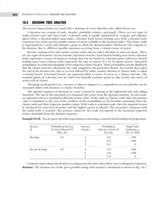
Example 4.9: Following is the data on daily earnings (in Rs.) of employees in a company:
Earnings : 50–70 70–90 90–110 110–130 130–150 150–170 170–190
No. of workers : 4 8 12 20 6 7 3
Calculate the first four moments about the point 120. Convert the results into moments about the
mean. Compute the value of γ1 and γ2 and comment on the result. [Delhi Univ., MBA, 1990, 2002]
Solution: Calculations for first four moments are shown in Table 4.5.
Table 4.5 Computation of First Four Moments
Class Mid-value Frequency d =
m 120
20
−
fd fd2
fd3
fd4
50–70 60 4 –3 –12 36 –108 324
70–90 80 8 –2 –16 32 –64 128
90–110 100 12 –1 –12 12 –12 12
110–130 120 20 0 0 0 0 0
130–150 140 6 1 6 6 6 6
150–170 160 7 2 14 28 56 112
170–190 180 3 3 9 27 81 243
60 –11 141 –41 825](https://image.slidesharecdn.com/businessstatisticsproblemsandsolutions-230910073954-6d42a210/85/Business-Statistics_-Problems-and-Solutions-pdf-127-320.jpg)
![117
SKEWNESS, MOMENTS, AND KURTOSIS
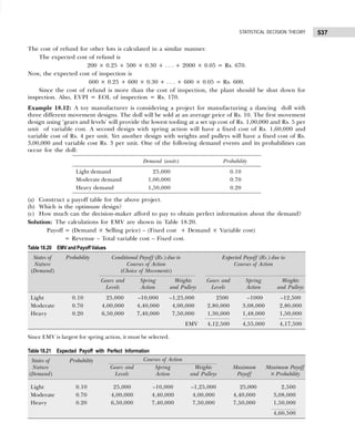
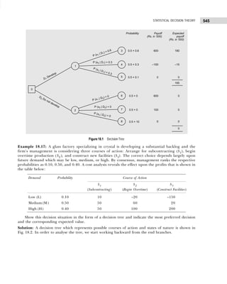
Example 4.12: Calculate the value of γ1 and γ2 from the following data and interpret them.
Profit (Rs. in lakh) : 10–20 20–30 30–40 40–50 50–60
Number of companies : 18 20 30 22 10
Comment on the skewness and kurtosis of the distribution. [Kumaon Univ., MBA, 1999]
Solution: Calculations for moments about an arbitrary constant value are shown in Table 4.8.
′
1
µ =
N
fd
h
×
∑
=
14
100
−
× 10 = – 1.4;
′
2
µ =
2
N
fd
∑
× h2
=
154
100
× 100 = 154;
′
3
µ =
2
N
fd
∑
× h3
=
62
100
−
× 1000 = – 620;
′
4
µ =
4
N
fd
∑
× h4
=
490
100
× 10,000 = 49,000.
The central moments are as follows:
µ2 = ′
2
µ – ( ′
1
µ )2
= 154 – (– 1.4)2
= 152.04;
µ3 = ′
3
µ – 3 ′
1
µ ′
2
µ + 2 ( ′
1
µ )3
= – 620 – 3 (– 1.4) (154) + 2 (– 1.4)3
= 21.312;
µ4 = ′
4
µ – 4 ′
1
µ ′
3
µ + 6 ′
2
µ ( ′
1
µ )2
– 3 ( ′
1
µ )3
=49,000 – 4 (– 1.4) (– 620) + 6 (154) (– 1.4)2
– 3 (– 1.4)3
= 47,327.51.
Karl Pearson’s relative measure of skewness and kurtosis are as follows:
Measure of skewness, γ1 =
σ
3
3
µ
= 3
3/2
2
µ
µ
= 3/ 2
21.312
(152.04)
=
21.312
1874.714
= 0.0114
Measure of kurtosis, β2 = 4
2
2
µ
µ
= 2
47,327.51
(152.04)
= 2.047
γ2 = β2 – 3 = 2.047 – 3 = – 0.953.
The value of γ1 = 0.0114 suggests that the distribution is almost symmetrical and γ2 = –0.953 (< 0)
indicates a platykurtic frequency curve.
Table 4.8 Calculations of Moments
Profit Mid-value Number of d = (m – 35)/10 f d f d2
f d3
f d4
(Rs. lakh) (m) Companies ( f )
10–20 15 18 – 2 – 36 72 – 144 288
20–30 25 20 – 1 – 20 20 – 20 20
30–40 35 ← A 30 0 0 0 0 0
40–50 45 22 1 22 22 22 22
50–60 55 10 2 20 40 80 160
100 – 14 154 – 62 490](https://image.slidesharecdn.com/businessstatisticsproblemsandsolutions-230910073954-6d42a210/85/Business-Statistics_-Problems-and-Solutions-pdf-131-320.jpg)
![BUSINESS STATISTICS: PROBLEMS AND SOLUTIONS
118
4.5 MISCELLANEOUS SOLVED EXAMPLES
Example 4.13: Calculate first four moments about the mean and also the value of β1 and β2 from the
following data:
Marks : 0–10 10–20 20–30 30–40 40–50 50–60 60–70
No. of
students : 8 12 20 30 15 10 5
[Kumaon Univ., MBA, 2001]
Solution: Calculations of first four moments and β1 and β2 are shown below in the table.
Marks Mid-point No. of d = (m – 35)/10 fd fd2
fd3
fd4
(m) Students
0–10 5 8 –3 –24 72 –216 648
10–20 15 12 –2 –24 48 –96 192
20–30 25 20 –1 –20 20 –20 20
30–40 35 30 0 0 0 0 0
40–50 45 15 +1 +15 15 +15 15
50–60 55 10 +2 +20 40 +80 160
60–70 65 5 +3 +15 45 +135 405
100 –18 240 –102 1440
Moments about arbitrary point A = 35 are origin (or point)
µ1
′ =
Σ −
× × −
18
= 10 = 1.8
100
fd
h
N
; µ2′=
Σ
× ×
2
2 240
= 100 = 240
100
fd
h
N
;
µ3′=
Σ −
× × −
3
3 102
= 1000= 1020
100
fd
h
N
; µ4′ =
Σ
× ×
4
4 1440
= 10000=144000
100
fd
h
N
.
Converting moments about arbitrary origin to moments about mean as follows:
µ2 = µ4′ – (µ1′)2
= 240 – (– 1.8)2
= 240 – 3.24 = 236.76,
µ3 = µ3′ – 3µ1′µ2′ + 2µ1′3
= – 1020 – 3 (1.8) (240) + 2 (– 1.8)3
= – 1020 + 1296 – 11.664 = 264.336,
µ4 = µ4′ – 4µ4′ µ3′ + 6(µ1′)2
µ2′ – µ1′4
= 144000 – 4 (– 1.8) (– 1020) + 6 (– 1.8)2
(240) – 3 (– 1.8)4
= 144000 – 7344 + 4665.6 – 31.4928 = 141290.11,
β1 =
2 2
3
3 3
2
(264.336)
= =0.005;
(236.76)
µ
µ
β2 = 4
2 2
2
141290.11
= = 2.521.
(236.76)
µ
µ
Example 4.14: From the following data calculate moments about
(i) assumed mean 25, (ii) actual mean, (iii) moments about zero.
Variable : 0–10 10–20 20–30 30–40
Frequency : 1 3 4 2 [M.G. Univ., B.Com., 1997]](https://image.slidesharecdn.com/businessstatisticsproblemsandsolutions-230910073954-6d42a210/85/Business-Statistics_-Problems-and-Solutions-pdf-132-320.jpg)
![119
SKEWNESS, MOMENTS, AND KURTOSIS
Solution: Calculations of first four moments about arbitrary origin are shown in the table below:
Variable Mid-point Frequency d = (m – 25)/10 fd fd2
fd3
fd4
(m)
0–10 5 1 –2 –2 4 –8 16
10–20 15 3 –1 –3 3 –3 3
20–30 25 ← A 4 0 0 0 0 0
30–40 35 2 1 2 2 2 2
10 –3 9 –9 21
µ1
′ =
Σ −
× × −
3
= 10 = 3
10
fd
h
N
; µ2′ =
Σ
× × ×
2
2 2
9 9
= (10) = 100 =90
10 10
fd
h
N
;
µ3′=
Σ −
× × −
3
3 9
= 1,000 = 900
10
fd
h
N
; µ4′ =
Σ
× ×
4
4 21
= 10,000 = 21,000
10
fd
h
N
.
Moments about Mean
µ1 = 0,
µ2 = µ2′ – (µ1′)2
= 90 – (– 3)2
= 81,
µ3 = µ3′ – 3µ1′µ2′ + 2µ1′3
= – 900 – 3 [(–3) (90)] + 3 (–3)3
= – 900 + 810 – 54 = – 144,
µ4 = µ4′ – 4µ4′ µ3′ + 6(µ1′)2
µ2′ – 3µ1′4
= 21,000 – 4 (– 3) (–900) + 6 (– 3)2
90 – 3 (–3)4
= 21,000 – 10,800 + 4,860 – 243 = 14,817.
Moments about Zero
ν1 = A + µ1′ = 25 – 3 = 22,
ν2 = µ2 – (ν1)2
= 81 + (22)2
= 565,
ν3 = ν3 – 3ν1ν2 – 2ν1
3
= – 144 + 3 (22) (565) – 2 (22)3
= – 144 + 37,290 – 21,296 = 15,850,
ν4 = µ4′ – 4ν4ν3 + 6ν1
2
ν2 + 3ν1
4
= 14817 + 4 (22) (15850) – 6 (22)2
(565)2
+ 3 (22)4
= 14817 + 1394800 – 1640760 + 702768 = 471625.
Example 4.15: Compute the coefficient of skewness and kurtosis based on the following data:
Variable (x) : 4.5 14.5 24.5 34.5 44.5 54.5 64.5 74.5 84.5 94.5
Frequency ( f ) : 1 5 12 22 17 9 4 3 1 1
[Punjab Univ., M.A., 2005]
Solution: Calculations of skewness and kurtosis are shown below:
Variable (x) Frequency (f) d = (x – 44.5)/10 fd fd2
fd3
fd4
4.5 1 –4 –4 16 –64 256
14.5 2 –3 –15 45 –135 405
24.5 12 –2 –24 48 –96 192
34.5 22 –1 –22 22 –22 22
44.5 ← A 17 0 0 0 0 0
54.5 9 1 9 9 9 9
64.5 4 2 8 16 32 64
74.5 3 3 9 37 81 243
84.5 1 4 4 16 64 256
94.5 1 5 5 25 125 625
75 –30 224 –6 2,072](https://image.slidesharecdn.com/businessstatisticsproblemsandsolutions-230910073954-6d42a210/85/Business-Statistics_-Problems-and-Solutions-pdf-133-320.jpg)
![BUSINESS STATISTICS: PROBLEMS AND SOLUTIONS
120
µ1′ =
–30
= = 0.4;
75
fd
N
Σ
− µ2′ =
Σ
−
2
224
= = 2.99
75
fd
N
;
µ3′ =
3
–6
= = 0.08;
75
fd
N
Σ
− µ4′ =
Σ
−
4
2,072
= = 27.63
75
fd
N
.
µ2 = µ2′ – (µ1′)2
= 2.99 – (– 0.4)2
= 2.99 – 0.16 = 2.83,
µ3 = µ3′ – 3µ1′µ2′ + 2(µ1′)3
= – 0.08 – 3 (–0.4) (2.99) + 2 (– 0.4)3
= 0.08 + 3.588 – 0.128 = 3.38,
µ4 = µ4′ – 4µ4′ µ3′ + 6µ1′2
µ2′ – 3(µ1′)4
= 27.63 – 4(– 0.4) (– 0.08) + 6 (– 0.4) (2.99) + 3 (– 0.4)4
= 27.63 – 0.128 + 2.87 – 0.077 = 30.295.
Skewness, β1 =
2 2
3
3 3
2
(3.38) 11.424
= = =0.504.
22.665
(2.8)
µ
µ
Kurtosis, β2 = 4
2 2
2
30.295 30.295
= = = 3.782.
8.01
(2.83)
µ
µ
Example 4.16: The first four central moments of distribution are 0, 2.5, 0.7, and 18.75. Comment on the
skewness and kurtosis of the distribution. 0[DelhiUniv.,B.Com.,(II),1990;KanpurUniv.,M.Com.,1993]
Solution: Given that µ1 = 0, µ2 = 2.5, µ3 = 0.7 and µ4 = 18.75. Thus, we get
Skewness, β =
2
3
3
2
µ
µ
=
2
3
(0.7)
=0.031
(2.5)
.
Since β1 = 0.031, the distribution is slightly skewed, that is, it is not perfectly symmetrical.
Testing Kurtosis
Kurtosis, β2 = 4
2
2
µ
µ
= 2
18.75 18.75
= = 3
6.25
(2.5)
.
Since β2 is exactly three, the distribution is mesokurtic (normal or symmetrical)
Example 4.17: Find the coefficient of skewness from the following information :
Different to two quartiles = 8; Mode = 11;
Sum of two quartiles = 22; Mean = 8. [Delhi Univ., B.Com.(H), 1997]
Solution: Using the Bowley’s coefficient of skew formula:
Skb =
+ −
−
3 1
3 1
2 Median
Q Q
Q Q
.
From the given information we get
Mode = 3 Median – 2 Mean
11 = 3 Median – 2 (8)
3 Median = 11 + 16 or Median = 9
Q3 + Q1 = 22, Q3 – Q1 = 8, Median = 9.
Hence, Skb =
22 2 (9)
= 0.5.
8
−
Example 4.18: From the data given below calculate the coefficient of variation :
Karl Pearson’s coefficient of skewness = 8; Arithmetic Mean = 86;
Median = 80. [Osmania Univ., B.Com., 1998]
Solution: Calculating first the value of standard deviation by using Karl Parson coefficient of skewness as
follows:](https://image.slidesharecdn.com/businessstatisticsproblemsandsolutions-230910073954-6d42a210/85/Business-Statistics_-Problems-and-Solutions-pdf-134-320.jpg)
![121
SKEWNESS, MOMENTS, AND KURTOSIS
Skp =
− Mode
X
σ
Mode = 3 Median – 2 X = 3 (80) – 2 (86) = 240 – 172 = 68
Skp = 42, X = 86, and Mo = 68.
Thus, Skp =
− Mode
X
σ
42 =
−
86 68
σ
or σ = 42.86
and hence CV = × = ×
42.86
100 100= 49.84
86
X
σ
per cent.
Example 4.19: Calculate the coefficient of skewness from the following data :
Mid-point : 15 20 25 30 35 40
Frequency : 12 18 25 24 20 21
[Jodhpur Univ., B.Com., 1997]
Solution: The calculation for mean, mode standard deviation are shown in Table 4.9.
Table 4.9 Calculations of Coefficient of Skewness
Mid-point Frequency d = (m – 25)/5 fd fd2
(m) f
15 12 –2 –24 48
20 18 –1 –18 18
25 ← A 25 0 0 0
30 24 1 24 24
35 20 2 40 80
40 21 3 63 189
120 85 359
Assuming A = 25. Then
X =
85
= 25 5= 25 3.542= 28.542
120
fd
A h
N
Σ
+ × + × +
σ =
2 2
359 85
5
120 120
fd fd
h
N N
Σ Σ
− × = − ×
= 2.992 .502 5=1.578 5=7.89
− × ×
Since highest frequency is 25, mode lies corresponding to mid-point 25, that is, in the class 22.5–27.5.
Mode = 1
1 1
2
m m
m m m
f f
l h
f f f
−
− +
−
+ ×
− −
L = 22.5, ∆1 = 25 – 18 = 7, ∆2 = 25 – 24 = 1, i = 5
Mo =
25 18
22.5 5
2 25 18 24
−
+ ×
× − −
=
7
22.5 5
8
+ ×
= 22.5 + 4.375 = 26.87
=
−
Mean Mode
σ
Skp =
28.542 26.875 1.667
= =0.211.
7.89 7.89
−](https://image.slidesharecdn.com/businessstatisticsproblemsandsolutions-230910073954-6d42a210/85/Business-Statistics_-Problems-and-Solutions-pdf-135-320.jpg)
![BUSINESS STATISTICS: PROBLEMS AND SOLUTIONS
122
Example 4.20: (a) The standard deviation of symmetrical distribution is 3. What must be the value of the
fourth moment about the mean in order that the distribution be mesokurtic? (b) If the first four moments
of distribution about the values 45 are equal to –4, 22, –117, and 560, determine the corresponding
moments (i) about the mean and (ii) about zero. [M.D. Univ., M.Com., 1999]
Solution: (a) For a mesokurtic distribution, β1 =
2
3
2
2
µ
µ
= 3; β2 = 4
2
2
µ
µ
.
Given that σ = 3, µ2 = σ2 = (3)2 = 9, β2 = 3, µ2 = 9. Hence,
β2(=3) = 4
2
(9)
µ
or µ4 = 243.
Thus, the fourth moment about mean is µ4 = 243, in order that distribution be mesokurtic.
(b) Given moments about an arbitrary origin 5 are µ1
′ = – 4, µ2′ = 22, µ3′ = – 117, µ4′ = 560.
Moments about Mean:
µ2 = µ2′ – (µ1′)2
= 22 – (– 4)2
= 22 – 16 = 6,
µ3 = µ3′ – 3µ1′µ2′ + 2(µ1′)3
= – 117 – 3 (– 4) (22) + 2 (–4)3
= – 117 + 264 – 128 = 19,
µ4 = µ4′ – 4µ1′µ3′ + 6µ2′(µ1′)2
– 3(µ1′)4
= 560 – 4 (– 4) (117) + (22) (– 4)2
– 3 (– 4)4
= 560 – 1872 + 2112 – 768 = 32.
Moments about Zero:
ν1 = 4 + µ1 = 4 = 6 + (1)2
= 7,
ν2 = µ1 + (ν1)2
= 19 + 3 (1) (7) – 2 (1)2
= 19 + 21 – 2 = 38,
ν3 = µ2 + 3ν1ν2 – 2ν1
2
= 32 + 4 (1) (38) – 6 (1)2
(7) + 3(1)4
,
ν4 = µ4 + 4ν1ν2 – 6(ν1)2
ν2 + 3ν1
4
= 32 + 152 – 42 + 3 = 145.
Example 4.21: The following data given are to an economist for the purpose of economic analysis. The
data refer to the length of a certain type of batteries.
n = 100, Σfd = 50, Σfd2
= 1970, Σfd3
= 2948, and Σfd4
= 86.752, in which d = (x – 48).
do you think that the distribution is platykurtic? [Delhi Univ., B.Com.(H), 1998]
Solution: For finding out whether the distribution is platykurtic or not, we need to calculate value of
Kurtosis, β2. For this, moments about origin are calculated as follows:
µ1′ =
50
= = 0.5
100
fd
N
Σ
; µ2′ =
2
1970
= =19.7
100
fd
N
Σ
;
µ3′ =
3
2948
= = 29.48
100
fd
N
Σ
; µ4′ =
4
86752
= =867.52
100
fd
N
Σ
.
µ2 = µ2′ – (µ1′)2
= 19.7 – (.5)2
= 19.45
µ3 = µ3′ – 3µ1′µ2
′ = 2 (µ1′)3 = 29.48 – 3(.5) (19.7) + 2(.5)3
= 29.48 – 29.55 + 0.25 = 0.18,
µ4 = µ4′ – 4µ1′µ3′ + 6µ1′2
– 3 (µ1′)4
= 867.82 – 4 (.5) (29.48) + 6 (19.7) (.5)2
– 3(.5)4
= 867.52 – 58.96 + 29.25 – 0.1875 = 837.6225.
Kurtosis, β2 = 4
2
2
µ
µ
= β2 = 2
837.6225 837.6225
= = 2.214( 3)
378.3025
(19.45)
< .
Since the value of β2 is less than 3, the distribution is platykurtic.](https://image.slidesharecdn.com/businessstatisticsproblemsandsolutions-230910073954-6d42a210/85/Business-Statistics_-Problems-and-Solutions-pdf-136-320.jpg)
![123
SKEWNESS, MOMENTS, AND KURTOSIS
Example 4.22: The first four moments of a distribution about arbitrary point x = 4 are 1, 4, 10, and 45.
Obtain the various characteristics of the distribution on the basis of the information given. Comment
upon the nature of the distribution. [B.A. (H) Eco., D.U., 1995]
Solution: Moments about arbitrary point x = 4 are µ3′ = 1, µ2′ = 4, µ3
′ = 10, µ4′ = 45, and A = 0. On the
basis of this information, the moments about mean and the values of arithmetic mean, standard deviation,
skewness, and kurtosis are determined as follows:
Moments about Mean:
µ1 = 1,
µ2 = µ2′ – (µ1′)2
= 4 – (1)2
= 3,
µ3 = µ3′ – 3µ1′µ2′ + 2(µ1′)3
= 10 – 3 (1) (4) + 2 (1)3
= 10 – 12 + 2 = 0,
µ4 = µ4′ – 4µ1′µ3′ + 6µ2′2
(µ2′)2
– 3 (µ1′)4
= 45 – 4 (1) (10) + 6 (4) (1)2
– 3 (1)4
= 45 – 40 + 24 – 3 = 26.
Mean, x = µ1′ = 1
Standard Deviation, σ = 2 = 3 =1.732
µ
Skewnesses, β1 =
2 2
3
2 2
2
(0)
= =0
(3)
µ
µ
Since β1 is zero, the distribution is symmetrical
Kurtosis, β2 = 4
2 2
2
26 26
= = = 2.89
9
(3)
µ
µ
.
Since β2 is less than 3, the distribution is platykurtic.
Example 4.23: Given Q1 = 18, Q3 = 25, Mode = 21, Mean = 18, find the coefficient of skewness.
[Kurukshetra Univ., M.A.(Eco.), 1997]
Solution: We are given Q1, Q2, and mode. But we need median for calculating skewness. The value of
median can be determined as follows:
Mode = 3 Median – 2X
21 = 3 Median – 2 × 18
3 Median = 57 or Median = 19.
Hence, Bowley’s coefficient of skewness is
Skb = 3 1
3 1
2 Med
Q Q
Q Q
+ −
−
=
25 18 2 (19) 43 38
= = 0.714.
254 18 7
+ − −
+
−
Example 4.24: Calculate coefficient of skewness by Karl Pearson’s method the value of β1 and β2 for the
following data:
Profits (Rs. Lakhs) : 10 – 20 20 – 30 30 – 40 40 – 50 50 – 60
No. of Companies : 18 20 30 22 10
[M.D. Univ., M.Com., 1998; Kumaun Univ., MBA, 2004]
Solution: Calculations for Karl Pearson’s coefficient of skewness are shown below:
Profit Mid-point Number of d = (m – 35)/10 fd fd2
fd3
fd4
(m) Companies
(f)
10–20 15 18 –2 –36 72 –144 288
20–30 25 20 –1 –20 20 –20 20
30–40 35 ← A 30 ← fm 0 0 0 0 0
40–50 45 22 1 22 22 22 22
50–60 55 10 2 20 40 80 160
100 –145 154 –62 490](https://image.slidesharecdn.com/businessstatisticsproblemsandsolutions-230910073954-6d42a210/85/Business-Statistics_-Problems-and-Solutions-pdf-137-320.jpg)
![BUSINESS STATISTICS: PROBLEMS AND SOLUTIONS
124
Mean, x =
fd
A h
N
Σ
+ × = 35 – ×
14
10
100
= 35 – 1.4 = 33.6.
Mode, Mo = 1
1 1
2
m m
m m m
f f
l h
f f f
−
− +
−
+ ×
− −
=
30 20
30 10
60 20 22
−
+ ×
− −
= 30 + 5.56 = 35.56.
Standard deviation, σ =
2
2
fd fd
h
N N
Σ Σ
− ×
=
−
− ×
2
154 14
10
100 100
= − ×
1.54 0.0196 10 = 1.233 × 10 = 12.33
SkP =
Mean – Mode
Standard Deviation
=
−
33.6 35.56
12.33
=
−1.96
12.33
= –0.159.
Moments, µ1′ =
Σfd
N
=
−14
100
= –0.14; µ2′ =
Σ 2
fd
N
=
154
100
= 1.54;
µ3′ =
Σ 3
fd
N
=
−62
100
= –0.62; µ4′ =
Σ 4
fd
N
=
490
100
= 4.9.
µ2 = ′ ′
− − − −
2 2
2 1
( ) =1.54 ( 0.14) =1.54 0.0196=1.5204
µ µ ,
µ3 = ′ ′ ′ ′
− + − + −
3
3 1 2 1
3 2 = 0.62 0.6468 0.005=0.0213
µ µ µ µ ,
µ4 = ′ ′ ′ ′ ′ ′
− + −
2 4
4 1 3 1 2 1
4 6 3
µ µ µ µ µ µ
= 4.9 – 4(–.14) (– .62) + 6(–0.14)2
(1.54) – 3 (–.14)4
= 4.9 – 0.3472 + 0.1811 + 0.0012 = 4.735,
1
β = =
3
3 2
2
0.0213 0.0213
= =0.0114.
1.8747
(1.5204)
µ
µ
β2 = 4
2 2
2
4.735 4.735
= = =2.048.
2.312
(1.5204)
µ
µ
Example 4.25: By using the quartiles find a measure of skewness for the following distribution.
Annual Sales (Rs. ’000) Number of Firms
Less than 20 30
Less than 30 255
Less than 40 465
Less than 50 580
Less than 60 634
Less than 70 644
Less than 80 650
Less than 90 665
Less than 100 680
[Bangalore Univ., B. Com., 1998]](https://image.slidesharecdn.com/businessstatisticsproblemsandsolutions-230910073954-6d42a210/85/Business-Statistics_-Problems-and-Solutions-pdf-138-320.jpg)
![125
SKEWNESS, MOMENTS, AND KURTOSIS
Solution: Determining simple frequencies with the given emulative frequencies as shown Table 4.10.
Table 4.10 Calculation of Q1, Q3, and Median
Annual Number of Cumulative
Sales Firms (f) Frequency
10 – 20 30 30
20 – 30 195 255
30 – 40 240 465
40 – 50 115 580
50 – 60 54 634
60 – 70 10 644
70 – 80 6 650
80 – 90 15 665
90 – 100 15 680
Q1 = Size of = =
680
th item 170th item
4 4
N
Q1 lies in the class 20 – 30, Q1 =
/ 4
N cf
l h
f
−
+ × = 20 +
−
×
170 30
10
195
= 20 + 7.18 = 27.18
Q3 = Size of
×
= =
3 680
3
th item 510th item
4 4
N
Q3 lies in the class 40 – 50, Q3 =
3 /4
N cf
l h
f
−
+ × = 40 +
−
510 465
115
× 10 = 40 + 3.9 = 43.9
Median = Size of
2
N
th item =
680
2
= 30th item
Median lies in the class 30–40
Med. = l +
/2
N cf
h
f
−
× = 30 +
−
340 225
240
× 10 = 30 + 4.79 = 34.79.
Hence, Skb = 3 1
3 1
2
Q Q Me
Q Q
+ −
−
=
+ −
−
340 27.18 2(34.79)
43.9 27.18
=
−
71.08 69.58 1.5
= = 0.09
16.72 16.72
.
Example 4.26: Calculate β1 and β2 from the following distribution and interpret the results.
Age Frequency Age Frequency
25–30 2 45–50 25
30–35 8 50–55 16
35–40 18 55–60 7
40–45 27 60–65 2
[M.D. Univ., M.Com., 1998; Kumaon Univ., MBA, 2000]
Solution: Calculations β1 and β2 are shown below:
Age Mid-point Frequency d = (m – 42.5)/5 fd fd2 fd3 fd4
(m) (f)
25–30 27.5 2 –3 –6 18 –54 162
30–35 32.5 8 –2 –16 32 –64 128
35–40 37.5 18 –1 –18 18 –18 18
40–45 42.5 ← A 27 0 0 0 0 0
45–50 47.5 25 1 25 25 25 25
50–55 52/5 7 3 21 63 189 567
60–65 62.5 2 4 8 32 128 512
105 46 252 334 1668](https://image.slidesharecdn.com/businessstatisticsproblemsandsolutions-230910073954-6d42a210/85/Business-Statistics_-Problems-and-Solutions-pdf-139-320.jpg)
![BUSINESS STATISTICS: PROBLEMS AND SOLUTIONS
126
Moments about arbitrary point A = 42.5
µ1′ =
Σ 46
=
105
fd
N
= 0.438; µ2′ =
Σ 2
252
=
105
fd
N
= 2.4;
µ3′ =
Σ 2
334
=
105
fd
N
= 3.181; µ4′ =
Σ 4
1668
=
105
fd
N
= 15.886.
Moments about mean
µ2 = µ2′ – (µ1′) = 2.4 – (0.438)2
= 2.4 – 0.192 = 2.208,
µ3 = µ3 – 3µ3′µ2′ + 2(µ1′)3
= 3.181 – 3(0.438) (2.4) – 2(0.438)3
= 3.181 – 3.1536 + 0.1681 = 0.1955,
µ4 = µ4′ – 4µ1′µ3 + 3(µ1′)4
= 15.886 – 4(0.438) (3.181) + 6(0.438)2
(2.4) – 3(0.438)4
= 15.886 – 5.573 + 2.763 – 0.111 = 12.965,
β1 =
2 3
3
3 2
2
(.1055)
=
(2.208)
µ
µ
= 0.0007; β2 =
4
2 2
2
12.965
= =2.66
(2.208)
µ
µ
.
Example 4.27: For a distribution Bowley’s coefficient of skewness is –0.56, Q1 is 16.4, and median
24.2. What is the coefficient of quartile deviation? [Delhi Univ., B.Com.(H), 1998]
Solution: Given Skb = –0.56, Q1 = 16.4, Med. = 24.2. Since
Skb =
+ −
−
3 1
3 1
2 Med.
Q Q
Q Q
,
–0.56 (Q3 – 16.4) = Q3 + 16.4 – 2(24.2)
–0.56Q3 + 9.184 = Q3 + 16.4 – 48.4
–1.56Q3 – Q3 = 16.4 – 48.4 – 9.184
–1.56Q3 = 41.184 or Q3 = 26.4.
Thus, QD =
− −
3 1 26.4 16.4
= =5
2 2
Q Q
.
Example 4.28: First three moments of a variable measured by point ‘2’ are gradually 1, 16, and –40.
Prove that mean is 3, variance is 15, and µ4 is –86 [Saurashtra Univ., B.Com., 2005]
Solution: The moments about arbitrary origin 2 are given as µ1′ = 1, µ2′ = 16, and µ3′ = –40. Hence,
Mean, x = A + µ1′ = 2 + 1 = 3
Variance, µ2 = µ2′ – µ1′2
= 16 –(1)3
= 15
µ3 = µ3′ – 3µ1′ µ2′ + 2µ1′3
= – 40 – 3(1) (16) + 2(1)3
= – 40 – 48 + 2 = – 86.
Example 4.29: The daily expenditure of the 100 families is given below:
Daily Expenditure : 0–20 20–40 40–60 60–80 80–100
No. of families : 13 ? 27 ? 16
Calculate the Karl Pearson’s coefficient of skewness.
Solution: Let the missing frequency for the class 20–40 be x. Then frequency for the class 60–80 shall be 100 – (x
+ 56) = 44 – x. Data are summarized as](https://image.slidesharecdn.com/businessstatisticsproblemsandsolutions-230910073954-6d42a210/85/Business-Statistics_-Problems-and-Solutions-pdf-140-320.jpg)
![127
SKEWNESS, MOMENTS, AND KURTOSIS
Expenditure Frequency Cumulative
(f) Frequency (cf)
0–20 13 13
20–40 x 13 + x
40–60 27 40 + x
60–80 (44 – x) 84
80–100 16 100
The mode value is calculated by using the formula
Mo = 1
1 1
2
m m
m m m
f f
l
f f f
−
− +
−
+
− −
,
where Mo = 44, which lies in the class 40–60. Hence,
44 =
27
40 20
27 17
x
x x
−
+ ×
− + −
4 = 2
27
20=(27 )
10
x
x
−
× −
or 27 – x = 2 or x = 25.
Thus the frequency for the class 20–40 is x = 25 and the frequency of the class 60–80 is 44–25 = 19. The
completed frequency distribution becomes
0–20 20–40 40–60 60–80 80–10
13 25 27 19 16
Calculation of Coefficient of Skewness
Daily Mid-point f d = (m – 50)/20 fd fd2
Expenditure (m)
0–20 10 13 –2 –26 52
20–40 30 25 –1 –25 25
40–60 50 27 0 0 0
60–80 70 19 1 19 19
80–100 90 16 2 32 64
100 0 160
Coeff. of Sk =
Mode
x −
σ
=
−
50 44 6
= = 0.237
25.3 25.3
,
where x =
0
=50 20=50
100
fd
A h
N
Σ
+ × + × ,
σ =
2 2
2
160 0
= 20= 25.3
100 100
fd fd
h
N N
Σ Σ
− × − ×
.
Example 4.30: Pearson’s coefficient of skewness for a distribution is 0.4 and coefficient of variance is 30%. Its
mode is 88. Find the mean and the median. [Delhi Univ., B.Com.(H), 1997]
Solution: Given that Skp = 0.4, Mode = 88, and Coeff. of variance (CV) is 30%. Calculations for mean and median
are as follows:
CV = =0.3 or =0.3 , and
x
x
σ
σ](https://image.slidesharecdn.com/businessstatisticsproblemsandsolutions-230910073954-6d42a210/85/Business-Statistics_-Problems-and-Solutions-pdf-141-320.jpg)
![BUSINESS STATISTICS: PROBLEMS AND SOLUTIONS
128
Skp =
− −
Mode 1 (Mo / )
=
/
x x
x
σ σ
0.4 =
1 (88/ ) 1 88
= 1
0.3 / 0.3
x
x x x
−
−
0.4 × 0.3 =
88
1
x
−
88
Mean
= 1 – .12 = .88
0.88 mean = 88 or mean =
88
=100
0.88
Mode = 3 Median – 2x
88 = 3 Median –2(100) or 3 Median = 288 or median = 96.
Hence mean and median are 100 and 96, respectively.
Example 4.31: A frequency distribution gives the following results:
(a) Coefficient of variation = 5;
(b) Standard deviation = 2;
(c) Karl Pearson’s coefficient of skewness = 0.5.
Find the mean and mode of the distribution. [Gulbarga Univ., B.Com., 1997]
Solution: Given CV = 5, σ = 2, and Karl Pearson’s coeff. of Sk = 0.5. Thus to find mean and mode use
the formula
CV = ×100
x
σ
5 =
2
100
x
× or 5 200
x = or x = 40.
Coeff. of Sk =
− Mode
x
σ
0.5 =
−
40 Mode
2
40 – Mode = 1 or Mode = 39.
Hence, mean of the distribution is 40 and mode is 39.
Example 4.32: Calculate Karl Pearson’s coefficient of skewness from the following data:
Marks more than : 5 15 25 35 45 55 65 75 85
No. of students : 120 105 96 85 72 58 42 12 0
[Kurukshetra Univ., MBA, 2004]
Solution: Based on the data, frequency table to calculate Karl Pearson coefficient of skewness is given
below:
Marks Mid-point Frequency d = (m – 50)/10 fd fd2
Cumulative
(m) (f.) Frequency (cf)
5–15 10 15 –4 –60 240 15
15–25 20 9 –3 –27 81 24
25–35 30 11 –2 –22 44 35
35–45 40 13 –1 –13 13 48
45–55 50 14 0 0 0 62
55–65 60 16 +1 +16 16 78
65–75 70 30 +2 +60 120 108
75–85 80 12 +3 +36 108 120
120 –10 622](https://image.slidesharecdn.com/businessstatisticsproblemsandsolutions-230910073954-6d42a210/85/Business-Statistics_-Problems-and-Solutions-pdf-142-320.jpg)
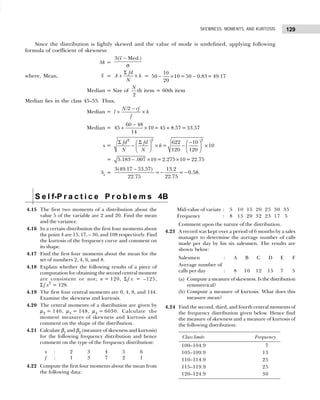
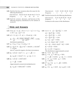
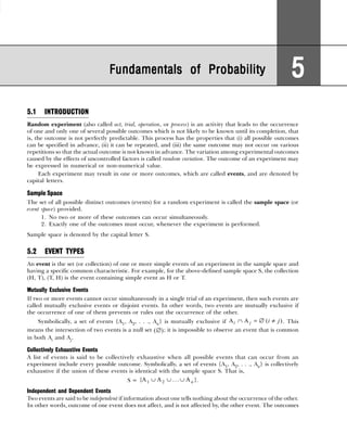
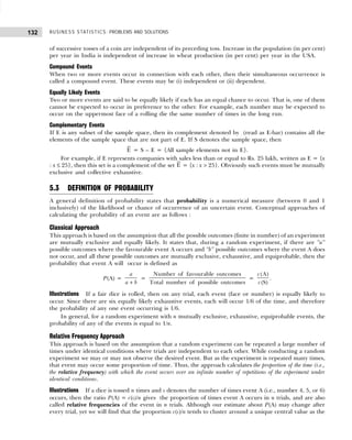
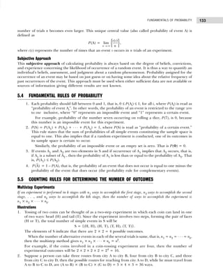
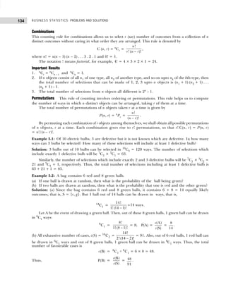
![135
FUNDAMENTALS OF PROBABILITY
Example 5.3: Tickets are numbered from 1 to 100. They are well shuffled and a ticket is drawn at
random. What is the probability that the drawn ticket has
(a) an even number? (b) the number 5 or a multiple of 5?
(c) a number which is greater than 75? (d) a number which is a square?
Solution: Since any of the 100 tickets can be drawn, exhaustive number of cases are c(S) = 100.
(a) Let A be the event of getting an even numbered tickets. Then, c(A) = 50, and hence
P(A) = 50/100 = 1/2.
(b) Let B be the event of getting a ticket bearing the number 5 or a multiple of 5, that is,
B = (5, 10, 15, 20, . . ., 95, 100),
which are 20 in number, c(B) = 20. Thus, P(B) = 20/100 = 1/5.
(c) Let C be the event of getting a ticket bearing a number greater than 75, that is,
C = {76, 77, . . ., 100},
which are 25 in number, c(C) = 25. Thus, P(C) = 25/100 = 1/4.
(d) Let D be the event of getting a ticket bearing a number which is a square, that is,
D = {1, 4, 9, 16, 25, 36, 49, 64, 81, 100},
which are 10 in number, c(D) = 10. Thus, P(D) = 10/100 = 1/10.
S e l f-P r a c t i c e P r o b l e m s 5A
5.1 Three unbiased coins are tossed. What is the probability
of obtaining
(a) all heads (b) two heads
(c) one head (d) at least one head
(e) at least two heads (f) all tails
5.2 A card is drawn from a well-shuffled deck of 52 cards.
Find the probability of drawing a card which is neither
a heart nor a king.
5.3 In a single throw of two dice, find the probability of
getting (a) a total of 11, (b) a total of 8 or 11, and (c)
same number on both the dice.
5.4 Five men in a company of 20 are graduates. If 3 men
are picked out of the 20 at random, what is the
probability that they are all graduates? What is the
probability of at least one graduate?
5.5 A bag contains 25 balls numbered 1 through 25.
Suppose an odd number is considered a “success”.
Two balls are drawn from the bag with replacement.
Find the probability of getting
(a) two successes (b) exactly one success
(c) at least one success (d) no successes
5.6 A bag contains 5 white and 8 red balls. Two drawings of
3 balls are made such that (a) the balls are replaced
before the second trial and (b) the balls are not replaced
before the second trial. Find the probability that the
first drawing will give 3 white and the second will give 3
red balls in each case.
[MD Univ., B.Com.; GND Univ., M.A., 1995;
Kerala Univ., M.Com., 1998]
5.7 Three groups of workers contain 3 men and one
woman, 2 men and 2 women, and 1 man and 3 women
respectively. One worker is selected at random from
each group. What is the probability that the group
selected consists of 1 man and 2 women?
[Nagpur Univ., M.Com., 1997;
Chennai Univ., M.Com., 2004]
5.8 What is the probability that a leap year, selected at
random, will contain 53 Sundays?
[Agra Univ., M.Com.; Kurukshetra Univ.,
M.Com., 1996; MD Univ., M.Com., 1998]
5.9 A university has to select an examiner from a list of 50
persons, 20 of them women and 30 men, 10 of them
knowing Hindi and 40 not, 15 of them being teachers
and the remaining 35 not. What is the probability of
the university selecting a Hindi-knowing woman
teacher? [Jammu Univ., M.Com., 1997]
Hints and Answers
5.1 (a) P(all heads) = 1/8
(b) P(two heads) = 3/8
(c) P(one head) = 3/8
(d) P(at least one head) = 7/8
(e) P(at least two heads) = 4/8 = 1/2
(f) P(all tails) = 1/8.
5.2 P(neither a heart nor a king) =
36
1
52
1
C
C
=
36
52
5.3 c(S) = 36; P(total of 11)
= 2/36 P(total of 9 or 11) = 7/36](https://image.slidesharecdn.com/businessstatisticsproblemsandsolutions-230910073954-6d42a210/85/Business-Statistics_-Problems-and-Solutions-pdf-149-320.jpg)
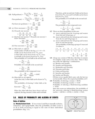
![137
FUNDAMENTALS OF PROBABILITY
This rule is expressed in the following formula
P(A or B) =
(A B) (A) (B)
(A B)
(S) (S)
n n n
P
n n
∪ +
∪ = =
=
(A) (B)
P(A) P(B)
(S) (S)
n n
n n
+ = + .
Let A be any event and A be the complement of A. Obviously A and A are mutually exclusive and
exhaustive events. Thus, either A occurs or it does not, is given by
P(A or A ) = P(A) + P(A ) = P(A) + {1 – P(A)} = 1
or P(A) = 1 – P(A ).
For example, if a dice is rolled, then the probability whether an odd number of spots occurs or does not.
(b) Partially Overlapping (or Joint) Events If events A and B are not mutually exclusive, it is possible for both
events to occur simultaneously. This means these events have some sample points in common. Such events
are also called joint (or overlapping) events as shown in Fig. 5.2.
This rule is expressed in the following formula:
P(A or B) = P(A) + P(B) – P(A and B)
or P(A ∪ B) = P(A) + P(B) – P(A ∩ B)
Figure 5.2 Partially Overlapping Events
Example 5.4: What is the probability that a randomly chosen card from a deck of cards will be either a
king or a heart.
Solution: Let event A and B be the king and heart in a deck of 52 cards, respectively. Then, it is given
that
Using the formula, we get
P(A or B) = P(A) + P(B) – P(A and B) =
4 13 1
52 52 52
+ − =
16
52
= 0.3077.
Example 5.5: Of 1000 assembled components, 10 have a working defect and 20 have a structural defect.
There is a good reason to assume that no component has both defects. What is the probability that
randomly chosen component will have either type of defect? [Delhi Univ., MBA, 2003]
Solution: Let events A and B be the component which has working defect and has structural defect,
respectively. Then it is given that
P(A) = 10/1000 = 0.01, P(B) = 20/1000 = 0.02 and P(A and B) = 0.
The probability that a randomly chosen component will have either type of defect is given by
P(A or B) = P(A) + P(B) – P(A and B) = 0.01 + 0.02 – 0.0 = 0.03.
Card Probability Reason
King P(A) = 4/52 4 kings in a deck of 52 cards
Heart P(B) = 13/52 13 hearts in a deck of 52 cards
King of heart P(A and (B) = 1/52 1 King of heart in a deck of 52 cards](https://image.slidesharecdn.com/businessstatisticsproblemsandsolutions-230910073954-6d42a210/85/Business-Statistics_-Problems-and-Solutions-pdf-151-320.jpg)
![BUSINESS STATISTICS: PROBLEMS AND SOLUTIONS
138
Example 5.6: A survey of 200 retail grocery shops revealed following monthly income pattern:
(a) What is the probability that a particular shop has monthly income under Rs. 20,000?
(b) What is the probability that a shop selected at random has either an income between Rs. 20,000 and
Rs. 30,000 or an income of Rs. 30,000 and more?
Solution: Let events A, B, and C represent the income under three categories, respectively.
(a) Probability that a particular shop has monthly income under Rs. 20,000 is P(A)=102/200=0.51.
(b) Probability that shop selected at random has income between Rs. 20,000 and Rs. 30,000 or Rs. 30,000
and more is given by
P(A or B) = P(A) + P(B) =
61 37
200 200
+ = 0.305 + 0.185 = 0.49.
Example 5.7: From a sales force of 150 persons, 1 will be selected to attend a special sales meeting. If 52
of them are unmarried, 72 are college graduates, and 3/4 of the 52 that are unmarried are college
graduates, find the probability that the sales person selected at random will be neither single nor a college
graduate.
Solution: Let A and B be the events that a salesperson selected is married and that he is a college
graduate, respectively. Given that P(A) = 52/150, P(B) = 72/150; P(A and B) = (3/4) (52/150)
= 39/150
The probability that a salesperson selected at random will be neither single nor a college graduate is
P( A ∩ B ) = 1 – P(A ∪ B) = 1 – {P(A) + P(B) – P(A ∩ B)}
= 1 –
52 72 39 13
150 150 150 30
+ − =
.
Example 5.8: From a computer tally based on employer records, the personnel manager of a large
manufacturing firm finds that 15 per cent of the firm’s employees are supervisors and 25 per cent of the
firm’s employees are college graduates. He also discovers that 5 per cent are both supervisors and college
graduates. Suppose an employee is selected at random from the firm’s personnel records, what is the
probability of
(a) selecting a person who is both a college graduate and a supervisor?
(b) selecting a person who is neither a supervisor nor a college graduate?
Solution: Let A and B be the events that the person selected is a supervisor and that he is a college
graduate, respectively. Given that P(A) = 15/100; P(B) = 25/100; P(A and B) = 5/100.
(a) Probability of selecting a person who is both a college graduate and a supervisor is
P (A and B) = 5/100 = 0.05.
(b) Probability of selecting a person who is neither a supervisor nor a college graduate is
P ( A and B ) =1 – P(A or B) = 1 – [P(A) + P(B) – P(A and B)]
=1 –
15 25 5
100 100 100
+ −
=
65
100
= 0.65.
Example 5.9: The probability that a contractor will get a plumbing contract is 2/3 and the probability
that he will not get an electrical contract is 5/9. If the probability of getting at least one contract is 4/5,
what is the probability that he will get both?
Solution: Let A and B denote the events that the contractor will get a plumbing and electrical contract,
respectively. Given that P(A) = 2/3; P(B) = 1 – (5/9) = 4/9; P(A ∪ B) = 4/5
Monthly Income (Rs.) Number of Shops
Under Rs. 20,000 102
20,000 to 30,000 061
30,000 and above 037](https://image.slidesharecdn.com/businessstatisticsproblemsandsolutions-230910073954-6d42a210/85/Business-Statistics_-Problems-and-Solutions-pdf-152-320.jpg)
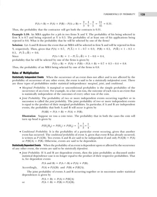
![BUSINESS STATISTICS: PROBLEMS AND SOLUTIONS
140
• Conditional Probability: Under statistical dependence, the conditional probability of event B,
given that event A has already occurred, is given by
P(B|A) =
P(A B)
P(A)
∩
.
Similarly, the conditional probability of A, given that event B has occurred, is
P(A|B) =
(A B)
(B)
P
P
∩
.
• Marginal Probability: The marginal probability of an event under statistical dependence is the
same as the marginal probability of an event under statistical independence. The marginal
probability of events A and B can be written as
P(A) = P(A ∩ B) + P(A ∩ B )
and P(B) = P(A ∩ B) + P( A ∩ B).
Example 5.11: The odds against student X solving a Business Statistics problem are 8 to 6 and odds in
favour of student Y solving the problem are 14 to 16.
(a) What is the chance that the problem will be solved if they both try independently of each other?
(b) What is the probability that none of them is able to solve the problem? [Delhi Univ., MBA, 1998]
Solution: Let A = The event that the first student solves the problem,
B =The event that the second student solves the problem.
P(A) =
6
8 6
+
=
6
14
and P(B) =
14
14 16
+
=
14
30
.
(a) Probability that the problem will be solved
= P (at least one of them solves the problem)
= P (A or B) = P(A) + P(B) – P(A and B)
= P(A) + P(B) – P(A) × P(B) [because the events are independent]
=
6 14 6 14
14 30 14 30
+ − × =
73
105
= 0.695.
(b) Probability that neither A nor B solves the problem
P (A and B) = P (A) × P (B) = [1 – P(A)] × [1 – P(B)] =
8 16
14 30
× =
32
105
= 0.305.
Example 5.12: The probability that a new marketing approach will be successful is 0.6. The probability
that the expenditure for developing the approach can be kept within the original budget is 0.50. The
probability that both of these objectives will be achieved is 0.30. What is the probability that at least one of
these objectives will be achieved. For the two events described above, determine whether the events are
independent or dependent.
Solution: Let A = The event that the new marketing approach will be successful
B = The event that the expenditure for developing the approach can be kept
within the original budget.
Given that P(A) = 0.60, P(B) = 0.50, and P(A ∩ B) = 0.30.
Probability that both events A and B will be achieved is given by
P(A ∪ B) = P(A) + P(B) – P(A ∩ B) = 0.60 + 0.50 – 0.30 = 0.80.
If events A and B are independent, then their joint probability is given by
P(A ∩ B) = P(A) × P(B) = 0.60 × 0.50 = 0.30.
Since this value is same as given in the problem, events are independent.](https://image.slidesharecdn.com/businessstatisticsproblemsandsolutions-230910073954-6d42a210/85/Business-Statistics_-Problems-and-Solutions-pdf-154-320.jpg)
![141
FUNDAMENTALS OF PROBABILITY
Example 5.13: A piece of equipment will function only when the three components A, B, and C are
working. The probability of A failing during one year is 0.15, that of B failing is 0.05, and that of C failing
is 0.10. What is the probability that the equipment will fail before the end of the year?
Solution: Given that
P(A failing) = 0.15; P(A not failing) = 1 – P(A)= 0.85;
P(B failing) = 0.05; P(B not failing) = 1 – P(B)= 0.95;
P(C failing) = 0.10; P(C not failing) = 1 – P(C)= 0.90;
Since all the three events are independent, the probability that the equipment will work is given
by
P( A ∩ B ∩ B ) = P( A ) × P(B ) × P( C ) = 0.85 × 0.95 × 0.90 = 0.726.
Probability that the equipment will fail before the end of the year is given by
P(A ∪ B ∪ C) = 1 – P( A ∩ B ∩ C ) = 1 – P( A ). P( B ). P( C )
= 1 – {0.85 × 0.95 × 0.90} = 1 – 0.726 = 0.274.
Example 5.14: A market research firm is interested in surveying certain attitudes in a small community.
There are 125 households broken down according to income, ownership of a telephone, and ownership
of a TV.
(a) What is the probability of getting a TV owner in a random draw?
(b) If a household has an income of over Rs. 8000 and is a telephone subscriber, what is the probability
that he owns a TV?
(c) What is the conditional probability of drawing a household that owns a TV, given that the household
is a telephone subscriber?
(d) Are the events ‘ownership of a TV’ and ‘telephone subscriber’ statistically independent? Comment.
[Himachal Univ., MBA, 1998]
Solution: (a) Probability of drawing a TV owner at random, P(TV owner) = 75/125 = 0.6
(b) There are 30(18 + 12) persons whose household income is above Rs. 8000 and are also telephone
subscribers. Out of these, 18 own TV sets. Hence, the probability of this group of persons having a
TV set is 18/30 = 0.6.
(c) Out of 75 ( 27 + 18 + 18 + 12) households who are telephone subscribers, 45 (27 + 18) households have
TV sets. Hence, the conditional probability of drawing a household that owns a TV given that the
household is a telephone subscriber is 45/75 = 0.6.
(d) Let A and B be the events representing TV owners and telephone subscribers respectively. The
probability of a person owning a TV, P(A)= 75/125. The probability of a person being a telephone
subscriber, P(B) = 75/125.
The probability of a person being a telephone subscriber as well as a TV owner is
P(A and B) = 45/125 = 9/25.
But P(A) × P(B) = (75/125) (75/125) = 9/25.
Since P(AB) = P(A) × P(B), we conclude that the events ‘ownership of a TV’ and ‘telephone subscriber’
are statistically independent.
Households with Annual Households with Annual Total
Income of Rs. 8000 or Less Income Above Rs. 8000
Telephone No Telephone No
Subscriber Telephone Subscriber Telephone
Own TV set 27 20 18 10 75
No TV set 18 10 12 10 50
Total 45 30 30 20 125](https://image.slidesharecdn.com/businessstatisticsproblemsandsolutions-230910073954-6d42a210/85/Business-Statistics_-Problems-and-Solutions-pdf-155-320.jpg)
![BUSINESS STATISTICS: PROBLEMS AND SOLUTIONS
142
Example 5.15: A company has two plants to manufacture scooters. Plant I manufactures 80 per cent of
the scooters and Plant II manufactures 20 per cent. In plant I, only 85 out of 100 scooters are considered
to be of standard quality. In plant II, only 65 out of 100 scooters are considered to be of standard quality.
What is the probability that a scooter selected at random came from plant I, if it is known that it is of
standard quality? [Madras Univ., M.Com, 1996]
Solution: Let A = The scooter purchased is of standard quality;
B = The scooter is of standard quality and came from plant I;
C = The scooter is of standard quality and came from plant II;
D = The scooter came from plant I.
The percentage of scooters manufactured in plant I that are of standard quality is 85 per cent of 80
per cent, that is, 0.85 × (80 ÷ 100) = 68 per cent or P(B) = 0.68.
The percentage of scooters manufactured in plant II that are of standard quality is 65 per cent of 20
per cent, that is, 0.65 × (20 ÷ 100) = 13 per cent or P(C) = 0.13.
The probability that a customer obtains a standard quality scooter from the company is 0.68 + 0.13
= 0.81.
The probability that the scooters selected at random came from plant I, if it is known that it is of
standard quality, is given by
P(D|A) =
( )
D and A
(A)
P
P
=
0.68
0.81
= 0.84.
Example 5.16: A husband and wife appear in an interview for two vacancies in the same post. The
probability of husband’s selection is 1/7 and that of wife’s selection is 1/5. What is the probability that
(a) both of them will be selected,
(b) only one of them will be selected, and
(c) none of them will be selected.
Solution: Let A and B be the events of the husband’s and wife’s selection, respectively. Given that P(A)
= 1/7 and P(B) = 1/5.
(a) The probability that both of them will be selected is
P(A and B) = P(A) P(B) = (1/7) × (1/5) = 1/35 = 0.029.
(b) The probability that only one of them will be selected is
P[(A and B ) or (B and A )] = P(A and B ) + P(B and A ) = P(A) P(B ) + P(B) P( A )
= P(A) [1 – P(B)] + P(B) [1 – P(A)]
=
1 1 1 1
1 1
7 5 5 7
− + −
=
1 4 1 6
7 5 5 7
× + ×
=
10
35
= 0.286.
(c) The probability that none of them will be selected is
P( A ) × P(B ) = (6/7)×(4/5) = 24/35 = 0.686.
Example 5.17: The odds that A speaks the truth is 3 : 2 and the odds that B speaks the truth is 5 : 3. In
what percentage of cases are they likely to contradict each other on an identical point?
[Delhi Univ., MBA, 1999]
Solution: Let X and Y denote the events that A and B speak truth, respectively. Given that
P(X) = 3/5; P( X ) = 2/5; P(Y) = 5/8; P( Y ) = 3/8.
The probability that A speaks the truth and B speaks a lie is (3/5) (3/8) = 9/40.
The probability that B speaks the truth and A speaks a lie is (5/8) (2/5) = 10/40.
So the compound probability is
9 10
40 40
+ =
19
40
.
Hence, percentage of cases in which they contradict each other is (19/40) × 100 = 47.5 per cent.](https://image.slidesharecdn.com/businessstatisticsproblemsandsolutions-230910073954-6d42a210/85/Business-Statistics_-Problems-and-Solutions-pdf-156-320.jpg)
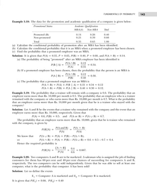
![BUSINESS STATISTICS: PROBLEMS AND SOLUTIONS
144
P(E1 and E2) or P(E1∩E2) = P(E1). P(E2) = 0.60 × 0.40 = 0.24.
Hence, the probability that computer A has been sold given that the salesman was able to sell at least
one computer is given by
P(E1|E1∪ E2) = 1 1 2
1 2
{E (E E )}
(E E )
P
P
∩ ∪
∪
= 1
1 2
(E )
(E E )
P
P ∪
= 1
1 2 1 2
(E )
(E )+ (E ) – (E E )
P
P P P ∩
=
0.60
0.60 0.40 0.24
+ −
= 0.789.
Example 5.21: A study of job satisfaction was conducted for four occupations: Cabin maker, lawyer,
doctor, and systems analyst. Job satisfaction was measured on a scale of 0–100. The data obtained are
summarized in the following table:
(a) Develop a joint probability table.
(b) What is the probability of one of the participants studied had a satisfaction score in 80’s?
(c) What is the probability of a satisfaction score in the 80’s, given the study participant was a doctor?
(d) What is the probability of one of the participants studied was a lawyer?
(e) What is the probability of one of the participants was a lawyer and received a score under 50?
(f) What is the probability of a satisfaction score under 50 given a person is a lawyer?
(g) What is the probability of a satisfaction score of 70 or higher? [Delhi Univ., MBA, 2003]
Solution: (a) Joint probability table is given below
(b) P(Satisfaction score in the 80’s) = 3/40.
(c) P(Satisfaction score in 80’s, given participant was a doctor) =
2/40
10/40
=
1
5
.
(d) P(Participant was doctor) = 10/40.
(e) P(Lawyer and score under 50) =
(Lawyer Score under 50)
(Score under 50)
P
P
∩
=
6
40
.
(f) P(Score under 50, Lawyer) =
(Score under 50 Lawyer)
(Lawyer)
P
P
∩
=
6/40
10/40
=
6
10
.
(g) P(Satisfaction score of 70 or higher) = P(Score of 70 and above) + P(Score of 80 and above)
=
8 3
40 40
+ =
11
40
.
Occupation Under 50 50–59 60–69 70–79 80–89
Cabin maker 0.000 0.050 0.100 0.075 0.250
Lawyer 0.150 0.050 0.025 0.025 0.250
Doctor 0.000 0.125 0.050 0.025 0.250
System analyst 0.050 0.025 0.100 0.075 0.250
Occupation Under 50 50–59 60–69 70–79 80–89 Total
Cabin maker 0 2 4 3 1 10
Lawyer 6 2 1 1 0 10
Doctor 0 5 2 1 2 10
Systems analyst 2 1 4 3 0 10
8 10 11 8 3 40](https://image.slidesharecdn.com/businessstatisticsproblemsandsolutions-230910073954-6d42a210/85/Business-Statistics_-Problems-and-Solutions-pdf-158-320.jpg)
![145
FUNDAMENTALS OF PROBABILITY
Example 5.22: A market survey was conducted in four cities to find out the preference for brand A soap.
The responses are shown below:
(a) What is the probability that a consumer selected at random preferred brand A?
(b) What is the probability that a consumer preferred brand A and was from Chennai?
(c) What is the probability that a consumer preferred brand A, given that he was from Chennai?
(d) Given that a consumer preferred brand A, what is the probability that he was from Mumbai?
[Delhi Univ., MBA, 2002; Kumaon Univ., MBA, 1999]
Solution: The information from responses during market survey is as follows:
Let X denote the event that a consumer selected at random preferred brand A. Then
(a) The probability that a consumer selected at random preferred brand A is
P(X) = 210/390 = 0.5398.
(b) The probability that a consumer preferred brand A and was from Chennai (C) is
P(X ∩ C) = 60/390 = 0.1538.
(c) The probability that a consumer preferred brand A, given that he was from Chennai is
P(X|C) =
(A C)
(C)
P
P
∩
=
60 / 390
100 / 390
=
0.153
0.256
= 0.597.
(d) The probability that the consumer belongs to Mumbai, given that he preferred brand A is
P(M|X) =
(M X)
(X)
P
P
∩
=
50 / 390
210 / 390
=
0.128
0.538
= 0.237.
Example 5.23: The personnel department of a company has records which show the following analysis
of its 200 engineers.
If one engineer is selected at random from the company, find
(a) the probability that he has only a bachelor’s degree;
(b) the probability that he has a master’s degree, given that he is over 40; and
(c) the probability that he is under 30, given that he has only a bachelor’s degree.
[Kumaon Univ., MBA, 1998]
Solution: Let A, B, C, and D denote the events that an engineer is under 30 years of age, 40 year of age,
has bachelor’s degree only, and has a master’s degree, respectively. Therefore,
(a) The probability of an engineer who has only a bachelor’s degree is
P(C) = 150/200 = 0.75.
Delhi Kolkata Chennai Mumbai Total
Yes 45 55 60 50 210
No 35 45 35 45 160
No opinion 5 5 5 5 20
Total 85 105 100 100 390
Delhi Kolkata Chennai Mumbai
Yes 45 55 60 50
No 35 45 35 45
No opinion 5 5 5 5
Age Bachelor’s Degree Only Master’s Degree Total
Under 30 90 10 100
30 to 40 20 30 50
Over 40 40 10 50
Total 150 50 200](https://image.slidesharecdn.com/businessstatisticsproblemsandsolutions-230910073954-6d42a210/85/Business-Statistics_-Problems-and-Solutions-pdf-159-320.jpg)
![BUSINESS STATISTICS: PROBLEMS AND SOLUTIONS
146
(b) The probability of an engineer who has a master’s degree, given that he is over 40 years, is
P(D|B) =
(D B)
(B)
P
P
∩
=
10 / 200
50 / 200
=
10
50
= 0.20.
(c) The probability of an engineer who is under 30 years, given that he has only bachelor’s degree, is
P(A|C) =
(A C)
(C)
P
P
∩
=
90 / 200
150 / 200
=
90
150
= 0.60.
S e l f-P r a c t i c e P r o b l e m s 5B
5.10 Mr. X has 2 shares in a lottery in which there are 2
prizes and 5 blanks. Mr. Y has 1 share in a lottery in
which there is 1 prize and 2 blanks. Show that the
chance of Mr. X’s success to that of Mr. Y’s is 15 : 7.
5.11 Explain whether or not each of the following claims
could be correct:
(a) A businessman claims that the probability that he
will get contract A is 0.15 and that he will get
contract B is 0.20. Furthermore, he claims that
the probability of getting A or B is 0.50.
(b) A market analyst claims that the probability of
selling ten million rupees of plastic A or five million
rupees of plastic B is 0.60. He also claims that the
probability of selling ten million rupees of A and
five million rupees of B is 0.45.
5.12 The probability that an applicant for a Management
Accountant’s job has a postgraduate degree is 0.3, he
has had some work experience as a Chief Financial
Accountant is 0.7, and that he has both is 0.2. Out of
300 applicants, approximately, what number would
have either a postgraduate degree or some
professional work experience?
5.13 A can hit a target 3 times in 5 shots; B, can do it 2 times
in 5 shots; C can do the same 3 times in 4 shots. They
fire a volley. What is the probability that 2 shots hit?
5.14 A problem in business statistics is given to five students,
A, B, C, D, and E. Their chances of solving it are 1/2, 1/
3, 1/4, 1/5, and 1/6 respectively. What is the probability
that the problem will be solved?
[Madras Univ., B.Com., 1996;
Kumaon Univ., MBA, 2000]
5.15 A husband and wife appear in an interview for two
vacancies for the same post. The probability of
husband’s selection is 1/7 and that of wife’s selection is
1/5. What is the probability that
(a) only one of them will be selected?
(b) both of them will be selected?
(c) none of them will be selected?
5.16 Three persons A, B, and C are being considered for
appointment as Vice-Chancellor of a university, and
whose chances of being selected for the post are in the
proportion 14 : 2 : 3 respectively. The probability that
A if selected, will introduce democratization in the
university structure is 0.3, and the corresponding
probabilities for B and C doing the same are
respectively 0.5 and 0.8. What is the probability that
democratization would be introduced in the university?
5.17 There are three brands, say X, Y, and Z, of an item
available in the market. A consumer chooses exactly
one of them for his use. He never buys two or more
brands simultaneously. The probabilities that he buys
brands X, Y, and Z are 0.20, 0.16, and 0.45, respectively.
(a) What is the probability that he does not buy any
of the brands?
(b) Given that a customer buys some brand, what is
the probability that he buys brand X?
5.18 There is 50-50 chance that a contractor’s firm, A, will
bid for the construction of a multistoreyed building.
Another firm, B, submits a bid and the probability is 3/
5 that it will get the job, provided that firm A does not
submit a bid. If firm A submits a bid, the probability
that firm B will get the job is only 2/3. What is the
probability that firm B will get the job?
5.19 Plant I of XYZ manufacturing organization employs 5
production and 3 maintenance foremen, plant II of
the same organization employs 4 production and 5
maintenance foremen. From any one of these plants,
a single selection of two foremen is made. Find the
probability that one of them would be a production
and the other a maintenance foreman.
[Bombay Univ., MMS, 1997]
5.20 If a machine is correctly set up, it will produce
90 per cent acceptable items. If it is incorrectly set up,
it will produce 40 per cent acceptable items. Past
experience shows that 80 per cent of the setups are
correctly done. If after a certain setup, the machine
produces 2 acceptable items as the first 2 pieces, find
the probability that the machine is correctly set up.
[Delhi Univ., B.Com., (H), 1998]
5.21 A firm plans to bid Rs. 300 per tonne for a contract to
supply 1,000 tonnes of a metal. It has two competitors
A and B. It assumes the probability of A bidding less
than Rs. 300 per tonne to be 0.3 and B’s bid to be less
than Rs. 300 per tonne to be 0.7. If the lowest bidder
gets all the business and the firms bid independently,
what is the expected value of the contract to the firm?](https://image.slidesharecdn.com/businessstatisticsproblemsandsolutions-230910073954-6d42a210/85/Business-Statistics_-Problems-and-Solutions-pdf-160-320.jpg)
![147
FUNDAMENTALS OF PROBABILITY
5.22 An investment consultant predicts that the odds against
the price of a certain stock going up during the next
week are 2 : 1 and odds in favour of the price remaining
the same are 1 : 3. What is the probability that the
price of the stock will go down during the next week?
5.23 An article manufactured by a company consists of two
parts A and B. In the process of manufacture of part
A, 9 out of 100 are likely to be defective. Similarly, 5
out of 100 are likely to be defective in the manufacture
of part B. Calculate the probability that the assembled
part will not be defective.
5.24 A product is assembled from three components X, Y,
and Z, the probability of these components being
defective is 0.01, 0.02, and 0.05, respectively. What is
the probability that the assembled product will not be
defective?
5.25 The daily production of a machine producing a very
complicated item gives the following probabilities for
the number of items produced: P(1) = 0.20, P(2) =
0.35, and P(3) = 0.45. Furthermore, the probability
of defective items being produced is 0.02. Defective
items are assumed to occur independently. Determine
the probability of no defectives during a day’s
production.
5.26 The personnel department of a company has records
which show the following analysis of its 200 engineers:
Age (Years) Bachelor’s Master’s Total
Degree only Degree
Under 30 90 10 100
30 to 40 20 30 50
Over 40 40 10 50
Total 150 50 200
If one engineer is selected at random from the
company, find
(a) the probability that he has only a bachelor’s
degree;
(b) the probability that he has a master’s degree given
that he is over 40;
(c) the probability that he is under 30, given that he
has only a bachelor’s degree.
[HP Univ., MBA; Kumaon Univ., MBA, 1998]
5.27 In a certain town, males and females form 50 per cent
of the population. It is known that 20 per cent of the
males and 5 per cent of the females are unemployed.
A research student studying the employment situation
selects unemployed persons at random. What is the
probability that the person selected is (a) male, (b)
female? [Delhi Univ. M. Com., 1999;
Kumaon Univ., MBA, 1990]
5.28 You note that your officer is happy in 60 per cent cases
of your calls. You have also noticed that if he is happy,
he accedes to your requests with a probability of 0.4,
whereas if he is not happy, he accedes to your requests
with a probability of 0.1. You call on him one day and
he accedes to your request. What is the probability of
his being happy? [HP
, Univ., MBA, 1996]
5.29 In a telephone survey of 1000 adults, respondents
were asked about the expenses on a management
education and the relative necessity of some form of
financial assitance. The respondents were classified
according to whether they currently had a child
studying in a school of management and whether they
thought that the loan burden for most management
students is too high, right amount, or too little. The
proportions responding in each category are given
below.
Too High Right Amount Too Little
(A) (B) (C)
Child studying
management (D) : 0.35 0.08 0.01
No child studying
management (E) : 0.25 0.20 0.11
Suppose one respondent is chosen at random from
this group. Then
(a) What is the probability that the respondent has a
child studying management?
(b) Given that the respondent has a child studying
management, what is the probability that he/she
ranks the loan burden as “too high”?
(c) Are events D and A independent? Explain.
5.30 In a colour preference experiment, eight toys are
placed in a container. The toys are identical except for
colour—two are red, and six are green. A child is asked
to choose two toys at random. What is the probability
that the child chooses the two red toys?
5.31 A survey of executives dealt with their loyalty to the
company. One of the questions was, “If you were given
an offer by another company equal to or slightly better
than your present position, would you remain with
the company?” The responses of 200 executives in
the survey cross-classified with their length of service
with the company are shown below:
Length of Service
Less than 1–5 6–10 More than Total
Loyalty 1 Year Years Years 10 Years
Would
remain : 10 30 05 75 120
Would
not remain : 25 15 10 30 080
What is the probability of randomly selecting an
executive who is loyal to the company (would remain)
and who has more than 10 years of service.](https://image.slidesharecdn.com/businessstatisticsproblemsandsolutions-230910073954-6d42a210/85/Business-Statistics_-Problems-and-Solutions-pdf-161-320.jpg)
![BUSINESS STATISTICS: PROBLEMS AND SOLUTIONS
148
Hints and Answers
5.10 Considering Mr. X’s chances of success.
A = event that 1 share brings a prize and 1 share goes
blank.
B = event that both the shares bring prizes.
C = event that X succeeds in getting atleast one prize
C = A ∪ B.
Since A and B are mutually exclusive,
P(C) = P(A ∪ B) = P(A) + P(B)
=
2 5
2 5
2 0
1 1
7 7
2 2
C C
C C
C C
×
×
+ .
Similarly, if D denotes the event that Y succeeds in
getting a prize, then we have
P(D) =
1
1
3
1
C
C
=
1
3
X’s chance of success: Y’s chance of success
=
15
21
:
1
3
= 15 : 7.
5.11 (a) P(A ∩ B) = – 0.15
(b) P(A) + P(B) = 1.05
5.12 Let A = Applicant has P.G degree;
B = Applicant has work experience;
Given P(A) = 0.3, P(B) = 0.7, and P(A ∩ B)
= 0.2. Therefore,
300 × P(A ∪ B) = 300[P(A) + P(B) – P(A ∩ B)] = 240
5.13 The required event that two shots may hit the target
can happen in the following mutually exclusive cases:
(a) A and B hit and C fails to hit the target
(b) A and C hit and B fails to hit the target
(c) B and C hit and A fails to hit the target
Hence, the required probability that any two shots hit
is given by P = P(i) + P(ii) + P(iii).
Let E1, E2, and E3 be the event of hitting the target by
A, B, and C respectively. Therefore,
P(i) = 1 2 3
(E E E )
P ∩ ∩
= P(E1) ⋅ P(E2) ⋅ 3
(E )
P
=
3 2 3
1
5 5 4
⋅ ⋅ −
=
6
100
P(ii) = 1 2 3
(E E E )
P ∩ ∩
=
3 2 3
1
5 5 4
−
=
27
100
P(iii) = 1 2 3
(E E E )
P ∩ ∩ =
3 2 3
1
5 5 4
−
=
12
100
Since all the three events are mutually exclusive
events, the required probability is given by
P(i) + P(ii) + P(iii) =
6 27 12
100 100 100
+ + =
9
20
5.14 P(problem will be solved)
= 1 – P(problem is not solved)
= 1 – P(all students fail to solve the problem)
= 1 (A B C D E)
P
− ∩ ∩ ∩ ∩
= 1 (A) (B) (C) (D) (E)
P P P P P
−
=
1 1 1 1 1
1 1 1 1 1 1
2 3 4 5 6
− − − − − −
=
1
1
6
− =
5
6
5.15 P(only one of them will be selected)
= (H W) (H W)
P ∩ ∪ ∩
= (H W) (H W)
P ∩ + ∩
= (H) (W) (H) (W)
P P P P
+
=
1 1 1 1
1 1
7 5 7 5
− + −
=
2
7
(b) P(both of them will be selected)
P(H ∩ W) = P(H) ⋅ P(W) =
1
35
(c) P(none of them will be selected)
(H W)
P ∩ = (H) P(W)
P ⋅ =
24
35
5.16 P(D) = Prob. of the event that democratization would
be introduced
= P[(A ∩ D) ∪ [(B ∩ D) ∪ (C ∩ D)]
= P[(A ∩ D) + P(B ∩ D) + P(C ∩ D)
= P(A) ⋅ P(D | A) + P(B) ⋅ P(D | B)
+ P(C)⋅P(D | C)
=
4 2 3
0.3 0.5 0.8
9 9 9
+ +
= 0.51
5.17 (a) P(customer does not buy any brand)
= [X Y Z]
P ∩ ∩ = 1 – P[(X ∪ Y ∪ Z]
= 1 – [P(X) + P(Y) + P(Z)]
= 1 – (0.20 + 0.16 + 0.45) = 0.19
(b) P(customer buys brand X) = P[X | (X ∪ Y ∪ Z)]
=
[X (X Y Z)]
(X Y Z)
P
P
∩ ∪ ∪
∪ ∪](https://image.slidesharecdn.com/businessstatisticsproblemsandsolutions-230910073954-6d42a210/85/Business-Statistics_-Problems-and-Solutions-pdf-162-320.jpg)
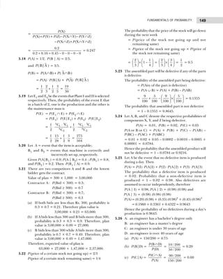
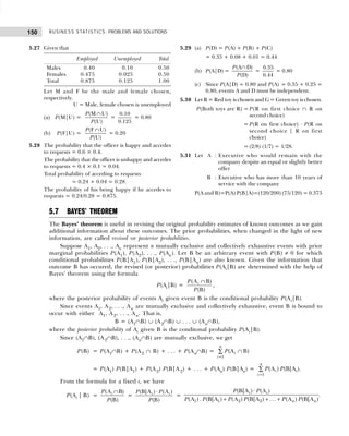
![151
FUNDAMENTALS OF PROBABILITY
Example 5.24: Suppose an item is manufactured by three machines X, Y, and Z. All the three machines
have equal capacity and are operated at the same rate. It is known that the percentages of defective items
produced by X, Y, and Z are 2, 7, and 12 per cent, respectively. All the items produced by X, Y, and Z are
put into one bin. From this bin, one item is drawn at random and is found to be defective. What is the
probability that this item was produced on Y?
Solution: Let A be the defective item. We know the prior probability of defective items produced on X, Y,
and Z, that is, P(X) = 1/3; P(Y) = 1/3; and P(Z) = 1/3. We also know that
P(A|X) = 0.02, P(A|Y) = 0.07, P(A|Z) = 0.12.
Now, having known that the item drawn is defective, we want to know the probability that it was
produced by Y. That is,
P(Y|A) =
(A|Y) (Y)
(X) (A|X)+ (Y) (A|Y)+ (Z) . (A|Z)
P P
P P P P P P
=
(0.07) · (1/ 3)
(1/ 3) (0.02) (1/ 3) (0.07) (1/ 3) (0.12)
+ +
= 0.33.
Example 5.25: Assume that a factory has two machines. Past records show that machine 1 produces
30 per cent of the items of output and machine 2 produces 70 per cent of the items. Further, 5 per cent of
the items produced by machine 1 were defective and only 1 per cent produced by machine 2 were defective.
If a defective item is drawn at random, what is the probability that the defective item was produced by
machine 1 or machine 2? [Kashmir Univ., M.Com., 2003]
Solution: Let A1 = Event of drawing an item produced by machine 1,
A2 = Event of drawing an item produced by machine 2,
and D = Event of drawing a defective item produced either by machine 1 or machine 2.
From the data in the problem we know that
P(A1) = 0.30, P(A2) = 0.70; P(D | A1) = 0.05, P(D | A2) = 0.1.
The data of the problem can now be summarized as under:
Here P(D) =
2
1
(D|A ) (A )
i i
i
P P
=
∑ = 0.05 × 0.30 + 0.01 × 0.70 = 0.22.
From the table above, the probability that the defective item was produced by machine 1 is 0.682 or
68.2 per cent and that by machine 2 is only 0.318 or 31.8 per cent. We may now say that the defective item
is more likely drawn from the output produced by machine 1.
Example 5.26: In a bolt factory, machines A, B, and C manufacture 25 per cent, 35 per cent and 40 per
cent of the total output, respectively. Of the total of their output, 5, 4, and 2 per cent are defective bolts.
A bolt is drawn at random and is found to be defective. What is the probability that it was manufactured
by machines A, B, or C? [Punjab Univ., M.Com.; Madurai Univ., M.Com., 1998]
Solution: Let, Ai (i = 1, 2, 3) be the event of drawing a bolt produced by machine A, B, and C, respectively.
From the data we know that
P(A1) = 0.25; P(A2) = 0.35; and P(A3) = 0.40
Event Prior Conditional Joint Probability Posterior (revised)
Probability Probability Event Probability
P(Ai ) P(D|Ai) P(Ai and D) P(Ai|D) P(Ai and D)
(1) (2) (3) (2) × (3)
A1 0.30 0.05 0.015 0.015/0.022 = 0.682
A2 0.70 0.01 0.007 0.007/0.022 = 0.318](https://image.slidesharecdn.com/businessstatisticsproblemsandsolutions-230910073954-6d42a210/85/Business-Statistics_-Problems-and-Solutions-pdf-165-320.jpg)
![BUSINESS STATISTICS: PROBLEMS AND SOLUTIONS
152
From the additional information we know that
B = the event of drawing a defective bolt.
Thus, P(B|A1) = 0.05; P(B|A 2) = 0.04; and P(B|A3) = 0.02.
The table of posterior probabilities can be prepared as under:
The above table shows the probability that the item was defective and produced by machine A is
0.362, by machine B is 0.406, and by machine C is 0.232.
Example 5.27: One card is drawn from a standard pack of 52. What is the probability that it is either a
king or a queen ? [Punjab Univ., B.Com., 1996; Chennai Univ., B.Com., 2006]
Solution: There are 4 kings and 4 queens in a pack of 52 cards. Therefore,
Probability that the card drawn is a king = 4/52
and Probability that the card drawn is a queen = 4/52.
Since the events are mutually exclusive, probability that the card drawn is either a king or a queen is
given by
P(king U Queen) =
4 4 8 2
= =
52 52 52 13
+ .
Example 5.28: Calculate the probability of picking a card that was a heart or a spade. Comment on your
answer. [Chennai Univ., B.Com., 2006]
Solution: The probability that a card will be both a heart and a spade is zero because each individual
card can be of one and only one of that type. Thus, intersection contains no outcomes since heart and
spade cannot simultaneously come in the same draw. Using the addition rule, we get
P (Heart or Spade) = P (heart) + P (spade) – P (heart and spade)
=
13 13 0 26 1
= =
52 52 52 52 2
+ − .
Example 5.29: A man wants to marry a girl having qualities: white complexion–the probability of getting
such a girl is one is twenty; handsome dowry–the probability of getting this is one in fifty; westernised
manners and etiquettes–the probability here is one in hundred. Find out the probability of his getting
married to such a girl when the possession of these three attributes is independent.
[Punjab Univ., B. Com., 1997; Kashmir Univ., M.Com., 2002]
Solution: Probability of a girl with white complexion 1/20 = 0.5;
Probability of a girl with handsome dowry 1/50 = 0.02;
Probability of a girl with westernised manners 1/100 = 0.01.
Since the events are independent, the probability of simultaneous occurrence of all these qualities
P(WC ∩ HD ∩ WM) = P(WC) × P(HD) × P(WM) =
1 1 1
=0.05 0.02 0.01=0.0001.
20 50 100
× × × ×
Event Prior Conditional Joint Probability Posterior Probability
Probability Probability
P(Ai) P(B|Ai) (2) × (3)
(1) (2) (3) (4) (5)
A1 0.25 0.05 0.0125 0.0125 ÷ 0.0345 = 0.362
A2 0.35 0.04 0.0140 0.014 ÷ 0.0345 = 0.406
A3 0.40 0.02 0.0080 0.008 ÷ 0.0345 = 0.232
Total 1.00 0.0345 1.000](https://image.slidesharecdn.com/businessstatisticsproblemsandsolutions-230910073954-6d42a210/85/Business-Statistics_-Problems-and-Solutions-pdf-166-320.jpg)
![153
FUNDAMENTALS OF PROBABILITY
Example 5.30: A bag contains 5 white and 3 black balls. Two balls are drawn at random one after the
other after the other without replacement. Find the probability that both balls drawn are black.
[Bhartidasan Univ., 2000]
Solution: Probability of drawing a black ball in the first attempt is
P(A) =
3 3
=
5 3 8
+
.
Probability of drawing the second ball given that the first ball drawn is black
P(B|A) =
2 2
=
5 2 7
+
.
The probability that both balls drawn are black is given by
P(A|B) = P (A) × P(B|A) =
3 2 3
= .
8 7 28
×
Example 5.31: A petrol pump proprietor sells on an average Rs. 80,000 worth of petrol on rainy days
and an average of Rs. 95,000 on clear days. Statistics from the Metrological Department show that the
probability is 0.76 for clear weather and 0.24 for rainy weather on coming Monday. Find the expected
value of petrol sale on coming Monday. [Karnataka Univ., B.Com., 1997]
Solution: The expected value of petrol sale on coming monday is given by
Expected sale = p1x1 + p2x2
= 0.24 (80,000) + 0.76 (95,000)
= 19,200 + 72,200 = Rs. 91,400.
Example 5.32: A bag contains 6 white, 4 red, and 10 black balls. Two balls are drawn at random. Find
the probability that they will both be black. [Chennai Univ., B.Com., 2006]
Solution: Total number of balls in the bag are 6 + 4 + 10 = 20.
Two balls can be drawn from 20 ball in 20
C2 =
20! 20 19
=
2!18! 2
×
.
Two balls can be drawn from 10 black balls in 10
C2 or =
20! 20 19
= = 45 days
2!18! 2
×
.
Thus, the probability that the two balls drawn at random are black is 45/190 = 0.237.
Example 5.33: A bag contains 8 white and 4 red balls. Five balls are drawn at random. What is the
probability that 2 of them are red and 3 white? [Chennai Univ., B.Com., 2006]
Solution: Total number of balls in the bag are 8 + 4 = 12.
Thus, 5 balls can be drawn from 12 balls in 12
C5 ways, 2 red balls can be drawn from 4 red in 4
C2
ways, and 3 white balls can be drawn from 8 white balls in 8
C3 ways.
• The number of favourable cases to draw red and white balls are 4
C2 × 8
C3 Hence, the required
probability is
P(2R and 3W) =
4 8
2 3
12
5
C C
C
×
=
14
= 0.424.
33
Example 5.34: One bag contains 4 white and 2 black balls. Another contains 3 white and 5 black balls. If
1 ball is drawn from each bag, find the probability that (a) both are white, (b) both are black, and (c) one
is white and one is black. [Madras Univ., B.Com., 2005]
Solution: (a) Probability of drawing a white ball from the first bag, P(W1) = 4/6.
Probability of drawing a white ball from the second bag, P(W2) = 3/8.
Since the events are independent, the probability that both the balls are white,
P(W1 and W2) =
4 3 1
= .
6 5 4
×](https://image.slidesharecdn.com/businessstatisticsproblemsandsolutions-230910073954-6d42a210/85/Business-Statistics_-Problems-and-Solutions-pdf-167-320.jpg)
![BUSINESS STATISTICS: PROBLEMS AND SOLUTIONS
154
(b) Probability of drawing a black ball from the first bag, P(B1) = 2/6.
Probability of drawing a black ball from the second bag, P(B2) = 5/8.
Probability that both are black, P(B1 and B2) =
2 5 5
= .
6 8 24
×
(c) That event ‘one is white one is black’ is the same as saying that ‘either first ball is white and second is
black or first ball is black the second is white.’ Hence,
Probability that one is white and one is black
P(W and B) = (W) × (B) + (W) (B)
P P P P =
4 5 2 3
6 8 6 8
+
=
13
.
24
Example 5.35: An article manufactured by a company consists of two parts A and B. In the process of
manufacture of part A, 9 out of 100 are likely to be defective. Similarly, 5 out of 100 are likely to be
defective in the manufacture of part B. Calculate the probability that the assembled part will not be
defective. [Kumaon Univ., MBA, 2002]
Solution: Since assembled part will be defective if any of the part is defective, probability of the assembled
part being defective.
= P Any of the part is defective] = P (A ∪ B)
= P (A) + P (B) – P (A ∩ B) =
9 5 9 5
100 100 100 100
+ − ×
= 0.09 + 0.05 – 0.0045 = 0.1355.
Hence, the probability that assembled part is not defective = 1 – 0.1355 = 0.8645.
Example 5.36: (a) Given that four airlines provide service between Delhi and Mumbai. In how many
distinct ways can a person select airlines for a trip from Delhi to Mumbai and back, if (i) he must travel
both the ways by the same airline and (ii) he travel from Delhi to Mumbai by one airline and returns by
another?
(b) 6 coins are tossed simultaneously. What is the probability that they will fall with 4 heads and 2 tails up?
(c) If A is the event of getting a prize on the first punch and B the event of getting the prize on the second
punch, calculate the probability of getting two prizes taking two punches on a punch board which
contains 20 blanks and five prizes?
(d) In how many ways can the word ‘PROBABILITY’ be arranged?
(e) What is the probability of getting a number greater than two with an ordinary dice?
[Rajasthan Univ., M.Com., 2005]
Solution: (a) (i) Since the person travels from Delhi to Mumbai and back by the same airline, he can select
any one airline out of the four airlines. Hence, the number of ways of selecting an airline is
4
C1 = 4.
(ii) Since the person travels from Delhi to Mumbai by one airline and returns by another so there are
four ways of selecting one airline from Delhi to Mumbai. Now there are three airlines only by which he
has to return. The number of ways of selecting an airline for returns is 3
C1 = 3.
Hence, the number of ways of selecting airlines for a trip from Delhi to Mumbai such that both ways
travels in different airlines 4 × 3 = 12.
(b) The probability of a head P(H) = 1/2 and P(Tail, T) = 1/2.
Since out of 6 coins any 4 coins will show head and the remaining 2 will show tail, the required
probability
P(H = 4) =
4 2
6
4
1 1 15
=
2 2 64
C
.
(c) First prizes can be won in 5 ways. Then from remaining 4 prizes, the second prize can be won in 4
ways. Thus, there are 5 × 4 = 20 ways of winning two prizes.](https://image.slidesharecdn.com/businessstatisticsproblemsandsolutions-230910073954-6d42a210/85/Business-Statistics_-Problems-and-Solutions-pdf-168-320.jpg)
![155
FUNDAMENTALS OF PROBABILITY
Since there are 25 punches on the punch board, there are 25 ways of selecting first punch. Also there
are 24 ways of selecting the second punch. Thus, there are 25 × 24 = 600 ways of selecting two punches.
Hence, probability of winning two prizes is 20/600 = 1/30
(d) There are 11 letters in which ‘B’ comes twice and also ‘l’ comes twice. If all the words were different,
then there was 11! ways of arranging them. Since 2 B’s are coming, these can be arranged in 2 ! × 2 !
ways.
Hence the total number of ways of arranging the word “probability” are
11!
= 9979200.
2 ! 2!
×
(e) In an ordinary dice 3, 4, 5, and 6 means the number greater than 2. Hence, the probability of getting
a number greater than 2 is 4/5 = 2/3.
Example 5.37: A can solve 90 per cent of the problems given in a book and B can solve 70 per cent. What
is the porbability that at least one of them will solve a problem selected at random?
[Kurukshetra, Univ., B.Com., 2000; M.D. Univ., M.Com., 2004]
Solution: Probability that A will not be able to solve the problem
(A)
P =
9 1
1
10 10
− = .
Probability that B will not be able to solve the problem
(B)
P =
7 3
1
10 10
− = .
Probability that none of them will be able to solve the problem
(A and B) = (A B)
P P ∩ =
1 3 3
=
10 10 100
× .
Hence the probability that at least one of them will solve the problem
P(A or B) = P(A ∪ B) =
3 97
1 =
100 100
− .
Example 5.38: A fair dice is tossed twice. Find the probability of getting a 4, 5, or 6 on the first toss and
a 1, 2, 3, or 4 on the second toss. [Chennai Univ., B.Com., 2006]
Solution: On the First Toss:
The probability of getting 4, 5, or 6 = 30(1/6) = 3/6 = 1/2.
Since the events are mutually exclusive and hence each probability of 1/6 may be added.
On the Second Toss:
With the same rule as in the first toss, the probability of getting a 1, 2, 3, or 4 = 4(1/6) = 4/6 = 2/3.
Example 5.39: A manufacturing firm produces steel pipes in three plants with daily production volumes
of 500, 1000, and 2000 units respectively. According to past experience, it is known that the fractions of
defective output produced by the three plants are respectively .005, .008, and .010. If a pipe is selected
from a day’s total production and found to be defective, find out
(a) from which plant the pipe comes?
(b) What is the probability that it came from the first plant?
[Hyderabad Univ., MBA, 2005; Delhi Univ., MBA, 2006]
Solution: (a) Given that
A1 : production volume of first plant = 500 units;
A2 : production volume of second plant = 1,000 units;
A3 : production volume of third plant = 2,000 units;
E : a defective item.
P (Ai |E) is the probability that the item is produced by the plant, given that the item is defective.
P ( )
i
A E
∩ is the probability that the items are produced by the ith plant are defective.](https://image.slidesharecdn.com/businessstatisticsproblemsandsolutions-230910073954-6d42a210/85/Business-Statistics_-Problems-and-Solutions-pdf-169-320.jpg)
![BUSINESS STATISTICS: PROBLEMS AND SOLUTIONS
156
Prior Probabilities
P (A1) =
500 1
=
500 1000 2000 7
+ +
; P (A2) =
1000 2
=
3500 7
; P (A3) =
2000 4
=
3500 7
P (E|A1) = 0.005; P (E|A2) = 0.008; P (E|A3) = 0.010.
Joint Probabilities
1
( )
P A E
∩ = 1 1
1
( ) ( | )= (0.005)=0.005/7
7
P A P E A
2
( )
P A E
∩ = 2 2
2
( ) ( | )= (0.008)=0.016 /7
7
P A P E A
3
( )
P A E
∩ = 3 3
4
( ) ( | )= (0.10)=0.040 /7
7
P A P E A
P (E) = Σ P (Ai) P (E|Ai) = 0.061/7.
Posterior Probabilities
P (A1|E) =
1 1
( ) 0.005/7 5
= =
( ) 0.061/7 61
P A E
P E
∩
P (A2|E)=
2 1
( ) 0.016 /7 16
= =
( ) 0.061/7 61
P A E
P E
∩
P (A3|E) =
3 1
( ) 0.040 /7 40
= =
( ) 0.061/7 61
P A E
P E
∩
.
Since value of P (A3|E) is more amongst posterior probabilities, it is then probable that the defective
item has been drawn from the output of the third plant.
Example 5.40: (a) A problem of statistics is given to two students A and B. The odds in favour of A
solving the problem are 6 to 9 and against B solving the problem 12 to 10. If A and B attempt, find the
probability of the problem being solved. [Delhi Univ., B.Com.(H), 2000]
Solution: Let A = problem can be solved by A;
B = problem can be solved by B.
Then based on the data given in the problem we can find following probabilities :
P(A) = 6 6
=
6 9 15
+
; (A)
P =
6 9
1 =
15 15
− ;
P(B) =
12 5
1 =
12 10 11
−
+
; (B)
P =
5 6
1 =
11 11
− .
(A and B)
P = (A) × (B)
P =
9 6 18
=
15 11 55
×
P(A or B) =
18 37
1 = =0.673
55 55
− .
Example 5.41: A committee of 4 people is to be appointed from 3 officers of the production department,
4 officers of the purchase department, 2 officers of the sales department, and 1 chartered accountant.
Find the probability of forming the committee in the following manner :
(a) There must be one from each category.
(b) It should have at least one from the purchase department.
(c) The chartered accountant must be on the committee.
[Kumaon Univ., M.Com., 1998; Madras Univ. B.Com., 2006)
Solution: Total number of officers = 3 + 4 + 2 + 1 = 10.](https://image.slidesharecdn.com/businessstatisticsproblemsandsolutions-230910073954-6d42a210/85/Business-Statistics_-Problems-and-Solutions-pdf-170-320.jpg)
![157
FUNDAMENTALS OF PROBABILITY
4 persons can be chosen from 10 in 10
C4 =
10! 10 9 8 7
= =210 ways
4! 6! 4 3 2 1
× × ×
× × ×
.
(a) One person can be chosen from each category in 4
C1 = 4, 3
C1 = 3, 2
C1 = 2, 1
C1 = 1 ways.
Then the probability of forming a committee having one officer from each category
=
4 3 2 1 24
= = 0.114.
210 210
× × ×
(b) Let P (A) be the probability of selecting at least one purchase officer. Then remaining four persons are
to be selected from six persons not belonging to the purchase department. This can be done in 6
C4 = 6
C2
= 6 × 5/(2 × 1) = 15 ways. Thus,
∴ P ( A ) =
15 1
=
210 14
and P (A) =
1 13
1 (A)=1 = .
14 14
P
− −
(c) If a chartered accountant is to be included in the committee, selecting of any 3 persons out of 9
persons can be done
9
C3=
9 8 7
=84 ways
3 2 1
× ×
× ×
.
Hence, the probability of a chartered accountant being on the committee is
84
=
210 5
2
.
Example 5.42: In a certain town, males and females form 50 per cent of the population. It is known that
20 per cent of the males and 5 per cent of the females are unemployed. A research student is studying the
employment person at random. What is the probability that the person selected is (a) male (b) female?
[Delhi Univ., M.Com., 2000; Kumaon Univ., MBA, 2005]
Solution: The data of the problem according to the sex and employment status is summarized as follows:
Employed Unemployed Total
Males 0.40 0.10 0.50
Females 0.475 0.025 0.50
Total 0.875 0.125 1.00
Let M and F denote a male and a female chosen for study, respectively. U denote male and female
chosen is unemployed.
(a) P (M|U) =
( ) 0.10
= = 0.80
( ) 0.125
P M U
P U
∩
.
(b) P (F|U) =
( ) 0.025
= =0.20
( ) 0.125
P F U
P U
∩
.
Example 5.43: You note that your officer is happy in 60 per cent cases of your calls. You have also
noticed that if he is happy, he accedes to your requests with a probability of 0.4, whereas if he is not
happy, he accedes to your requests with a probability of 0.1. You call on him one day and he accedes to
your request. What is the probability of his being happy?
Solution: Let A and B officer is happy and accedes to request, respectively.
Then probability of officer being happy and accedes to request P(A and B) = P(A) × P(B) = 0.60.4 = 0.24.
Probability of officer not being happy and acceding to request (A and B) = (A) × (B) = 0.4 × 0.1 = 0.04
P P P .
Probability that he is unhappy and accedes to your requests = .4 × .1 = .04.
Thus, probability of the officer acceding to request becomes 0.24 + 0.04 = 0.28.
The probability of his being happy if he accedes to request = 0.24/0.28 = 0.857.](https://image.slidesharecdn.com/businessstatisticsproblemsandsolutions-230910073954-6d42a210/85/Business-Statistics_-Problems-and-Solutions-pdf-171-320.jpg)
![BUSINESS STATISTICS: PROBLEMS AND SOLUTIONS
158
Example 5.44: A certain production process produces items that are 10 per cent defective. Each item is
inspected before supplying to customers but the inspector incorrectly classifies an item 10 per cent of the
time. Only items classified as good are supplied. If 820 items have been supplied in all, how many of them
are expected to be defective?
Solution: Given that
P(D) = 10/100 = 0.1
Also, P(G|D) = 10/100 = 0.1
Hence, P(G) = 1 – P(D) = 1 – 0.1 = 0.9 and P(G|G) = 1 – P (G|D) = 1 – 0.1 = 0.9.
Hence,
P(D|G) =
(D). (G|D)
(D). (D|D)+ (G). (G|G)
P P
P P P P
=
0.1 0.1 0.001 1
= = = 0.012.
0.1 0.1 0.9 0.9 0.82 82
×
× + ×
Example 5.45: A manufacturing firm produces pipes in two plants I and II with daily production 1500
and 2000 pipes respectively. The fraction of defective pipes produced by two plants I and II are 0.006
and 0.008 respectively. If a pipe selected at random from that day’s production is found to be defective,
what is the chance that it has come from plant I or plant II? [Univ. of Kashmir, M.Com., 2006]
Solution: A1 and A2 pipe manufactured at plant I and II, respectively, then E = a defective pipe.
P (A1) = Probability that a pipe is manufactured in plant I
=
1,500 3
=
1,500 2,000 7
+
.
P (A2) = Probability that a pipe is manufactured in plant II
=
2,000 4
=
1,500 2,000 7
+
.
Then P(E|A1) = 0.006 and P(E|A2) = 0.008
P(E|A1) = 1
1
(E A )
(A )
P
P
∩
or P(E ∩ A1) = P(A1) × P(E|A1) = (3/7)10.006 = 0.01817
P(E|A2) = 2
2
(E A )
(A )
P
P
∩
or P(E ∩ A2) = P(A2) × P(E|A2) = (4/7)10,0081 = 0.032/7.
Probability that the defective pipe has come from plant I or plant II is given by
P(A1|E) = 1 1 1
i i
(A E) (A ) (E|A ) 0.018/7
= =
(E) SP(A ) (E|A ) 0.018/7+0.032/7
P P P
P P
∩
= 0.018/10.018 + 0.032) = 0.36
P(A2|E) = 2 2 2
i i
(A E) (A ) (E|A ) 0.032
= = = 0.64
(E) (A ) (E|A ) 0.050
P P P
P P P
∩
Σ
The calculations prove that the pipe probability has come from plant II.
Example 5.46: A box contains 4 white and 6 black balls. Two balls are drawn out together. What is the
probability that both are black?
Solution: Total number of balls in the box = 4 + 6 = 10.
The number of ways (combinations) in which two balls can be drawn together out of 10 balls:
n(S) = 10
C2 = ×
×
10 9
2 1
= 45 ways.](https://image.slidesharecdn.com/businessstatisticsproblemsandsolutions-230910073954-6d42a210/85/Business-Statistics_-Problems-and-Solutions-pdf-172-320.jpg)
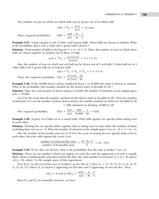
![BUSINESS STATISTICS: PROBLEMS AND SOLUTIONS
160
P(E1 ∪ E2) = P(E1) + P(E2) =
1 1 2
.
6 18 9
+ =
Hence, required probability = Probability of non-occurrence of both E1 and E2
= 1 – P(E1 ∪ E2) = 1 –
2 7
9 9
= .
Example 5.51: From a pack of caro one card is selected at random. What is the probability that the card
is a spade, a court, or a deuce?
Solution: We know that in a pack there are 52 cards out of which 13 are spades, 12 are court, and 4 are
deuce.
Let A1, A2, and A3 be the events of drawing a spade, a court, and a deuce card respectively. If S be the
sample space, then obviously n(S) = 52.
Also n(A1) = 13, n(A2) = 12, and n(A3) = 4. Here the events A2 and A3 are mutually exclusive, but the
events A1 and A2 or A1 and A2 are not. Thus,
A2 ∩ A3 = φ, [because A2, A3 are mutually exclusive]
or n(A2 ∩ A3) = 0
and n(A1 ∩ A2) = number of elements common in A1 and A2
= 3, [there are three court cards in spade]
n(A1 ∩ A3) = number of elements common to A1 and A3
= 1 [there is only one deuce of spade]
and n(A1 ∩ A2 ∩ A3) = number of elements common to A1, A2, A3
= 0 [there is no element common to all].
Hence, required probability = Probability that either A1 or A2 or A3 happens
= P(A1 ∪ A2 ∪ A2)
= P(A1) + P(A2) + P(A2) – P(A1 ∩ A2) – P(A1 ∩ A2) – P(A2 ∩ A3) +
P(A1 ∩ A2 ∩ A3)
= – 1 2 2 3 1 2 2
( ) ( ) ( )
( ) ( ) ( )
n A A n A A n A A A
n S n S n S
∩ ∩ ∩ ∩
− +
=
13 12 4 3 1 0 0
52 52 52 52 52 52 52
+ + − − − + =
25
52
.
Example 5.52: Two dice are thrown at a time. Let E1 be the event of getting 6 on the first dice and E2 that
of getting 1 on the second dice. Are the events E1 and E2 independent?
Solution: Any one of the numbers 1, 2, 3, 4, 5, 6 can appear on each dice. Thus combining the numbers
appearing on one dice with those appearing on the other, we get 6 × 6 = 36 outcomes. For example (3,
4) is one of these 6 outcomes which shows that 3 is appearing on the first dice and 4 on the second.
Thus, for this experiment n(S) = 36, where S is the sample space and
E1 = event of getting 6 on the first die
= {(6, 1), (6, 2), (6, 3), (6, 4), (6, 1), (6, 6)}
E2 = event of getting 1 on the second die
= {(1, 1), (2, 1), (3, 1), (4, 1), (5, 1), (6, 1)}.
Also, n(E1) = 6, n(E2) = 6 and E1 ∩ E2 = {(6, 1)} which gives n(E1 ∩ E2) = 1.
Now P(E1) = 1
( ) 6 1
;
( ) 36 6
n E
n S
= = P(E2) = 2
( ) 6 1
( ) 36 6
n E
n S
= =
and P(E1 ∩ E2) = 1 2
( ) 1
( ) 36
n E E
n S
∩
= .
Evidently P(E1 ∩ E2) = (1/36) = (1/6) × (1/6) = P(E1) P(E2). Hence, events E1 and E2 are independent.](https://image.slidesharecdn.com/businessstatisticsproblemsandsolutions-230910073954-6d42a210/85/Business-Statistics_-Problems-and-Solutions-pdf-174-320.jpg)
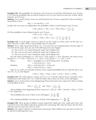
![BUSINESS STATISTICS: PROBLEMS AND SOLUTIONS
162
(a) girl, boy, boy, (b) boy, girl, boy, and (c) boy, boy, girl, where in (a) way the girl is chosen from first
group and one boy each from second and third groups of children.
Let E1, E2, and E3 be the events selecting the children as given in the ways (a), (b) and (c) respectively.
Then
P(E1) = probability of choosing one girl from first group, one boy from
second group, and one boy from third group
= ( ) ( )
3 2 3 3 1 3 9
× × = × × =
3+1 2+1 1+3 4 2 4 3
.
Similarly, P(E2) = probability of choosing one boy from first group, one girl from
second group, and one boy from third group
= ( ) ( )
1 2 3 1 1 3
3 1 2 1 1 3 4 2 4
× × = × ×
+ + +
=
3
.
32
P(E3) = probability of choosing one body from first group, one boy from
second group, and one girl from third group
= ( ) ( )
1 2 1 1 1 3
.
3 1 2 1 1 3 4 2 32
× × = × =
+ + +
Since these events E1, E2, and E3 are mutually exclusive, the required probability of one of these
events to happen:
P(E1) + P(E2) + P(E2) = 9 3 1 13
.
32 32 32 32
+ + =
Example 5.57: Ten coins are thrown simultaneously. Find the probability of getting at least 7 heads.
Solution: If p and q be the chances respectively of getting and not getting a head in the throw of a coin,
then p = 1
2
and q = 1
2
.
The required probability of getting at least seven heads = sum of the probabilities of getting 7, 8, 9,
and 10 heads:
=
10 10
10
7
1 1
2 2
r r
r
r
C
−
=
∑
=
10 10
10
10 10
7 7
1 1
2 2
r
r r
r r
C C
= =
=
∑ ∑
=
10
10 10 10 10
7 3 9 10
1
2
C C C C
+ + +
=
10
10 10 10 10
2 8 1 9
1
,
2
C C C C
+ + +
[n
Cr = n
Cn– 1]
=
10 9 8 10 9
1 10
1
32 32 3 2 1 2 1 1
× × ×
+ + +
× × × ×
= 1 176 11
[120 45 10 1]
32 32 32 32 64
+ + + = =
× ×
.
Example 5.58: Six dice are thrown 729 times. How many times do you expect at least 3 dice to show 5 or
6?
Solution: The probability of throwing 5 or 6 by a dice: 1/6 + 1/6 = 1/3.
Probability of showing 5 or 6 by at least 3 dice
= sum of the probabilities of showing 5 or 6 by 3, 4, 5, and 6 dice](https://image.slidesharecdn.com/businessstatisticsproblemsandsolutions-230910073954-6d42a210/85/Business-Statistics_-Problems-and-Solutions-pdf-176-320.jpg)
![163
FUNDAMENTALS OF PROBABILITY
=
−
=
−
∑
6
6
8
1 1 1
,
3 3 3
r r
n
r
r
C =
−
=
∑
6
6
6
9
1 2
3 3
r r
r
r
C
=
3 3 4 2 4 1 6
6 6 6 6
3 5 6
1 2 1 2 1 2 1
3 3 3 3 3 3 3
r
C C C C
+ + +
=
6
6 3 6 2 6 6
2 1 6
1
[ (2) (2) (2) ],
3
C C C C
+ + +
[n
Cr = n
Cn–r]
= [ ]
1 233 233
160 60 12 1
27 27 27 27 729
+ + + = =
× ×
.
Expected number out of 729 throws: 729 × 233
729
= 233.
Example 5.59: In a hand at whist (a game at cards played by four persons) what is the probability that
four kings are held by a specified player?
Solution: Each player gets 13 cards out of 52 cards in the pack. In this case the specified player is to get
4 kings and the remaining 9 cards in two hand are to be out of the remaining 48 cards of the pack.
The four kings can be selected in two ways and the remaining 9 cards in 48
c9 ways.
Also the total number of ways in which the specified player can get 13 cards out of 52 = 52
c13.
The required probability =
×
=
4 48 48
4 9 9
52 52
13 13
c c c
c c
.
Example 5.60: A and B throw alternately with a pair of ordinary dice. A wins if he throws six before B
throws seven and B wins if we throws seven before A throws six. If A begins, find his chance of winning.
Solution: There are five ways of throwing a total of six with a pair of ordinary dice and these are (1, 5),
(2, 4), (3, 3), (1, 2), and (5, 1) where (2, 4) means 2 shown by one dice and 4 by the other. Also the possible
number of throws with two dice is 6 × 6, that is, 36.
The probability of throwing a total of six with a pair of dice = ( )
5
36
and the probability not throwing a six = 1 – ( )
5 31
=
36 36
.
Similarly, there are six ways of throwing a total of seven with a pair of dice and these are (1, 6), (2, 5),
(3, 4), (4, 3), (5, 2), and (6, 1) as before. Thus, the probability of throwing a total of seven with a pair of
dice: ( ) ( )
6 1
36 6
= and not throwing a seven: 1 – ( )
1 5
=
6 6
.
Now A begins to throw the dice and the probability of his winning in the first throw is 5
36
and that
of not winning is 31
36
.
If A fails to throw a six, B gets a chance to throw and the probability of his winning in his first chance
(after A fails to win) is 31 1
=
36 6
.
If B fails to win in his first throw (i.e., both A and B fail to win in their first chance), then A gets the
second chance to throw. Now the probability that both A and B fail to win in their first chance:
31 5 5
36 6 36
× × .
Also, if A fails in second chance also, then the probability of B winning in the second chance:
( ) ( ) ( ) ( )
31 5 31 1
.
36 6 36 6
× × × [A and B have both failed in first chance and A in second chance too].](https://image.slidesharecdn.com/businessstatisticsproblemsandsolutions-230910073954-6d42a210/85/Business-Statistics_-Problems-and-Solutions-pdf-177-320.jpg)
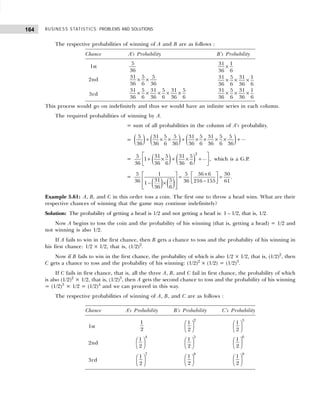
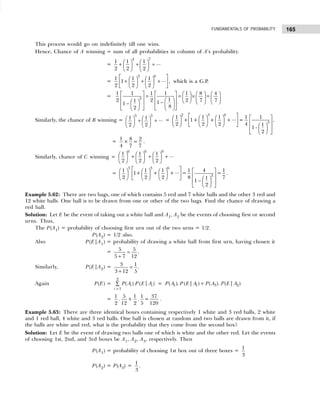
![BUSINESS STATISTICS: PROBLEMS AND SOLUTIONS
166
Also P(E|A1) = probability of drawing one white and the other red ball from the first box, when it
has already been chosen
=
1 3 3 1 1
× + × =
4 3 4 3 2
.
[Probability of drawing 1st ball white and 2nd ball red from 1st box which contains 4 balls in all = 1/
4 × 3/4 and that of 1st ball red and 2nd ball white from the same box = 3/4 × 1/3].
Similarly, P(E|A2) =
2 1 1 2 2
× + × =
3 2 3 2 3
and P(E|A2) =
4 3 3 4 4
× + + =
7 6 7 6 7
.
Hence, required probability = P(A2|E)
=
2 2 2 2
3
1
( ). ( | ) ( ). ( | )
=
( ) ( ) ( | )
t i
i
P A P E A P A P E A
P E A A P E A
=
∑
= 2 2
1 1 2 2 3 1
( ) ( | )
( ) ( | ) ( ) | ) ( ) ( | )
P A P E A
P A P E A P A P E A P A P E A
+ +
=
(1/3)(2/2) (2/3) (2/3) 28
= = =
1 1 1 2 1 4 1 2 4 7 3 73
× + × + × + +
3 2 3 2 3 7 2 2 7 4 8
Example 5.64: There are three coins, identical in appearance, one of which is ideal and the other two
biased with probabilities 1/3 and 2/3 respectively for a head. One coin is taken at random and tossed
twice; if a head appears both times, what is the probability that the ideal coin was chosen?
Solution: Let A1 be the event of choosing the 1st coin which is ideal, that is, with probability 1/2 for a
head turning up, A2 be the event of choosing the coin with probability 1/3 for a head turning up, and A3
that of choosing the third coin with probability 2/3 for a head turning up. Let E be the event of head
appearing when the selected coin is tossed w times. Then we have
P(A1) = choosing 1st coin out of three coins
= 1
3
= P(A2) = P(A3).
Also, P(E|A1) = probability of head of appearing in each of the two tosses when
1st coin is selected
=
1 1 1
2 2 4
× = .
Similarly, P(E|A2) =
1 1 1
3 2 9
× = and P(E|A2) = 2 2 4
3 3 9
× = .
The required probability P(A1|E) =
1 1 1 1
3
1
.( ) ( | ) ( ) ( | )
=
( ) ( ) ( | )
i i
i
P A P E A P A P E A
P E P A P E A
=
∑
,
=
1 1
1 2 2 2 2
( ) ( | )
( ) ( | ) ( ) ( | ) ( ) ( | )
P A P E A
P A P E A P A P E A P A P E A
+ +
=
( ) ( ) ( )
1 1 1
1 36 9
3 4 4
1 1 4
1 1 1 1 1 4 4 29 29
4 9 9
3 4 3 9 3 0
×
= = × =
+ +
× + × + ×
.](https://image.slidesharecdn.com/businessstatisticsproblemsandsolutions-230910073954-6d42a210/85/Business-Statistics_-Problems-and-Solutions-pdf-180-320.jpg)
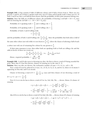
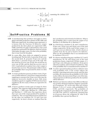
![169
FUNDAMENTALS OF PROBABILITY
5.32 Let A1, A2, and A3 = production volume of plant I, II,
and III, respectively.
E = defective steel pipe
P(A1) = 500/3500 = 0.1428;
P(A2) = 1000/3500 = 0.2857;
P(A3) = 2000/3500 = 0.5714
P(E | A1) = 0.005, P(E | A2) = 0.008,
and P(E | A3) = 0.010.
P(A1 ∩ E) = P(A1) P(E | A1)
= 0.1428 × 0.005 = 0.0007;
P(A2 ∩ E) = P(A2) P(E | A2)
= 0.2857 × 0.008 = 0.0022
P(A3 ∩ E) = P(A3) P(E | A3)
= 0.5714 × 0.010 = 0.057
P(E) = P(A1 ∩ E) + P(A2 ∩ E) + P(A3 ∩ E)
= 0.0007 + 0.0022 + 0.057 = 0.0599
(a) P(A1|E) = 1
(A E)
(E)
P
P
∩
=
0.0007
0.0599
= 0.0116
P(A2|E) = 2
(A E)
(E)
P
P
∩
=
0.0022
0.0599
= 0.0367;
P(A3|E) = 3
(A E)
(E)
P
P
∩
=
0.057
0.0599
= 0.951
Since P(A3 | E) is highest, the defective steel pipe has
most likely come from the third plant
(b) P(A1|E) = 1
(A E)
(E)
P
P
∩
= 1 1
(A ) (E|A )
(E)
P P
P
=
(500 / 3500) 0.005
0.0599
×
= 0.0119
5.33 Let A, B, and C = mail processed by first, second, and
third clerk, respectively
E = mail containing error
Given P(A) = 0.40,
P(B) = 0.35, and P(C) = 0.25
P(E | A) = 0.04, P(E | B) = 0.06,
and P(E | C) = 0.03
∴ P(A | E) =
(A) (E|A)
(E)
P P
P
=
(A) (E|A)
(A) (E|A)+ (B) (E|B)+ (C) (E|C)
P P
P P P P P P
=
0.40× 0.04
0.40 (0.04)+ 0.35 (0.06)+ 0.25 (0.03)
= 0.36
Similarly, P(B|E) = [P(B) P(E|B)]/P(E) = 0.47
P(C|E) = [P(C) P(E|C)]/P(E) = 0.17
5.34 P(D) = Probability of defective item = 0.1; P(classified
as good | defective) = 0.1
∴ P(G) = Probability of good item
= 1 – P(D) = 1 – 0.1 = 0.9
P(classified as good | good)
= 1 – P(classified as good | defective)
= 1 – 0.1 = 0.9
∴ P(defective | classified as good)
=
(D) (classified as good|defective)
[ (D) (classified as good|D)
+ (G) (classified as good|G)]
P P
P P
P P
⋅
⋅
=
0.1 0.1
0.1 0.1 0.9 0.9
×
× + ×
=
0.01
0.82
= 0.012.
5.35 (a) 0.20 (b) 0.20 (c) 0.60
5.36 P(A) = 0.37, P(B) = 0.40, P(C) = 0.23
5.37 P(Z) = 0.6639
5.38 P(A) = 0.012
5.39 P(A | H) = 0.3130
Hints and Answers](https://image.slidesharecdn.com/businessstatisticsproblemsandsolutions-230910073954-6d42a210/85/Business-Statistics_-Problems-and-Solutions-pdf-183-320.jpg)
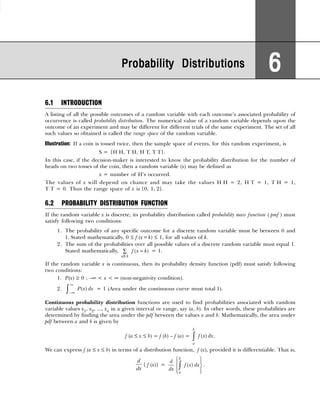
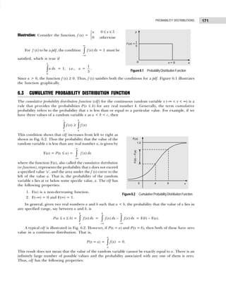
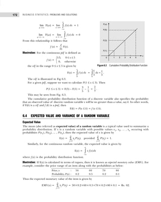
![173
PROBABILITY DISTRIBUTIONS
Variance and Standard Deviation
The expected value measures the central tendency of a probability distribution, while variance determines
the dispersion or variability to which the possible random values differ among themselves.
The variance, denoted by Var(x) or σ 2
, of a random variable x is the squared deviation of the individual
values from their expected value or mean. That is,
Var(x) = E[(x – µ)2
] = E(xj – µ)2
P(xj), for all j.
= E[(x2
– 2x µ + µ2
)] = E(x2
) – 2 µ E(x) + µ2
= E(x2
) – µ2
where E(x2
) = 2
1
( )
n
j
j
j
x P x
=
∑ and µ =
1
( )
n
j j
j
x P x
=
∑
Standard deviation (σx) = Var( )
x = 2
1
( ) ( )
n
j j
j
x P x
=
−
∑ µ .
Example 6.1: A doctor recommends a patient to take a particular diet for 2 weeks and there is equal
chance for the patient to lose weight between 2 kgs and 4 kgs. What is the average amount the patient is
expected to lose on this diet?
Solution: If x is the random variable, then probability density function is defined as
f (x) =
1
, 2 4
2
0, otherwise
x
< <
The amount the patient is expected to lose on the diet is
E(x) =
4
4 2
2
2
1
2 4
x
x dx
=
∫ = 2 2
1
(4) (2)
4
−
= 3 kg.
Example 6.2: From a bag containing 3 red balls and 2 white balls, a man is to draw two balls at random
without replacement. He gains Rs. 20 for each red ball and Rs. 10 for each white one. What is the
expectation of his draw.
Solution: Let x be the random variable denoting the number of red and white balls in a draw. Then x can
take up the following values.
P(x = 2 red balls) =
3
2
5
2
C
C
=
3
10
P(x = 1 red and 1 white ball) =
3 2
1 1
5
2
C C
C
×
=
3
5
P(x = 2 white balls) =
2
2
5
2
C
C
=
1
10
.
Thus, the probability distribution of x is
Hence, expected gain is E(x) = 40×(3/10) + 30×(3/5) + 20×(1/10) = Rs. 32.
Variable : 2R 1R and 1W 2W
Gain, x : 40 30 20
Probability, P(x): 3/10 3/5 1/10](https://image.slidesharecdn.com/businessstatisticsproblemsandsolutions-230910073954-6d42a210/85/Business-Statistics_-Problems-and-Solutions-pdf-187-320.jpg)
![BUSINESS STATISTICS: PROBLEMS AND SOLUTIONS
174
Example 6.3: Under an employment promotion programme, it is proposed to allow sale of newspapers
inside buses during off-peak hours. The vendor can purchase newspapers at a special concessional rate of
Rs 1.25 per copy against the selling price of Rs. 1.50. Any unsold copies are, however, a dead loss. A
vendor has estimated the following probability distribution for the number of copies demanded.
How many copies should be ordered so that his expected profit will be maximum?
Solution: Profit per copy = Selling price – Purchasing price = 1.50 – 1.25 = Rs. 0.25. Thus,
Expected profit = Number of copies × Probability × Profit per copy.
The calculations of expected profit are shown in Table 6.1.
Maximum profit of Rs. 140 is obtained when he stocks 17 copies of the newspaper.
Example 6.4: In a cricket match played to benefit an ex-player, 10,000 tickets are to be sold at Rs. 500.
The prize is a Rs. 12,000 fridge by lottery. If a person purchases two tickets, what is his expected gain?
Solution: The gain, say x, may take one of two values: he will either lose Rs. 1,000 (i.e., gain will be
–Rs. 1,000) or win Rs. (12,000–1,000) = Rs. 11,000, with probabilities 9,998/10,000 and 2/10,000,
respectively. The probability distribution for the gain x is given below:
The expected gain will be
µ = E(x) = Σx P(x) = –1000×(9,998/10,000)+11000×(2/10,000) = –Rs. 997.6.
The result implies that if the lottery were repeated an infinitely large number of times, average or expected
loss will be Rs. 997.6.
Example 6.5: A market researcher at a major automobile company classified households by car ownership.
The relative frequencies of households for each category of ownership are shown below:
Calculate the expected value and standard deviation of the random variable and interpret the result.
[Delhi Univ., MBA, 2003]
Number of copies : 15 16 17 18 19 20
Probability : 0.04 0.19 0.33 0.26 0.11 0.07
Table 6.1 Calculations of Expected Profit
Number of Probability Profit per Expected Profit
Copies Demanded Copy (Rs.) (Rs.)
(1) (2) (3) (4) = (1) × (2) × (3)
15 0.04 0.25 15
16 0.19 0.25 76
17 0.33 0.25 140
18 0.26 0.25 117
19 0.11 0.25 52
20 0.07 0.25 35
x P(x)
– Rs. 1000 9,998/10,000
Rs. 11000 2/10,000
Number of cars Relative
Per Household Frequency
0 0.10
1 0.30
2 0.40
3 0.12
4 0.06
5 0.02](https://image.slidesharecdn.com/businessstatisticsproblemsandsolutions-230910073954-6d42a210/85/Business-Statistics_-Problems-and-Solutions-pdf-188-320.jpg)
![175
PROBABILITY DISTRIBUTIONS
Solution: The necessary calculations required to calculate expected and standard deviation of a random
variable, say x, are shown in Table 6.2.
Expected value, µ = E(x) = ∑ x P(x) = 1.80. This value indicates that there are on an average 1.8 cars
per household.
Variance, σ 2
= ∑ x2
P(x) – [E(x)]2
= 4.44 – (1.80)2
= 4.44 – 3.24 = 1.20
Standard deviation, σ = 2
σ = 1.20 = 1.095 cars.
Example 6.6: The owner of a ‘Pizza Hut’ has experienced that he always sells between 12 and 15 of his
famous brand ‘Extra Large’ pizzas per day. He prepares all of them in advance and stores them in the
refrigerator. Since the ingredients go bad within one day, unsold pizzas are thrown out at the end of each
day. The cost of preparing each pizza is Rs. 120 and he sells each one for Rs. 170. In addition to the usual
cost, it costs him Rs. 50 per pizza that is ordered but cannot be delivered due to insufficient stock. If
following is the probability distribution of the number of pizzas ordered each day, then how many ‘Extra
Large’ pizza should he stock each day in order to minimize expected loss.
Solution: The loss matrix for the given question is shown in Table 6.3.
Since expected loss of Rs. 88 is minimum corresponding to a stock level of 13 pizza, the owner
should stock 13 ‘Extra Large’ pizzas each day.
Example 6.7: A company introduces a new product in the market and expects to make a profit of Rs. 2.5
lakh during the first year if the demand is ‘good’; Rs. 1.5 lakh if the demand is ‘moderate’; and a loss of
Rs. 1 lakh if the demand is ‘poor.’ Market research studies indicate that the probabilities for the demand
to be good and moderate are 0.2 and 0.5, respectively. Find the company’s expected profit and the
standard deviation.
Solution: Let x be the random variable representing profit in three types of demand. Thus, x may assume
the values
Table 6.2 Calculations of Expected Value and Standard Deviation
Number of Cars Relative x × P(x) x2
× P(x)
Per Household x Frequency, P(x)
0 0.10 0.10 0.00
1 0.30 0.30 0.30
2 0.40 0.80 1.60
3 0.12 0.36 1.08
4 0.06 0.24 0.96
5 0.02 0.10 0.50
1.80 4.44
Number of pizza demanded : 12 13 14 15
Probability : 0.40 0.30 0.20 0.10
Table 6.3 Pizza Ordered
Pizza Ordered
12 13 14 15
Probability → 0.40 0.30 0.20 0.10 Expected Loss
Pizza Stocked ↓
12 – 100 200 300 100
13 120 – 100 200 88
14 240 120 – 100 142
15 360 240 120 – 240](https://image.slidesharecdn.com/businessstatisticsproblemsandsolutions-230910073954-6d42a210/85/Business-Statistics_-Problems-and-Solutions-pdf-189-320.jpg)
![BUSINESS STATISTICS: PROBLEMS AND SOLUTIONS
176
x1 = Rs. 2.5 lakh when demand is good,
x2 = Rs. 1.5 lakh when demand is moderate, and
x3 = Rs. 1 lakh when demand is poor.
Since these events (demand pattern) are mutually exclusive and exhaustive,
P(x1)+P(x2)+P(x3) = 1 or 0.2 + 0.5 + P(x3) = 1 or P(x3) = 0.3.
Hence, the expected profit is given by
E(x) = 2.5 × 0.2 + 1.5 × 0.5 + (– 1) × 0.3 = Rs. 0.95 lakh.
Also, E(x2
) = x P x x P x x P x
1
2
1 2
2
2 3
2
3
( ) ( ) ( )
+ +
= (2.5)2
× 0.2 + (1.5)2
× 0.5 + (– 1)2
× 0.3 = Rs. 2.675 lakh.
Thus, S.D.(x) = Var( )
x = 2 2
E( ) [E( )]
x x
− = 2
2.675 (0.95)
− = Rs. 1.331 lakh.
S e l f-P r a c t i c e P r o b l e m s 6A
6.1 Anil company estimates the net profit on a new product
it is launching to be Rs. 30,00,000 during the first year
if it is ‘successful’; Rs. 10,00,000 if it is ‘moderately
successful’; and a loss of Rs. 10,00,000 if it is
‘unsuccessful’. The firm assigns the following
probabilities to its first year prospects for the product:
Successful: 0.15, moderately successful: 0.25. What
are the expected value and standard deviation of first
year net profit for this product?
[Delhi Univ., MBA, 2003]
6.2 A box contains 12 items of which 3 are defective. A
sample of 3 items is selected at random from this box.
If x represents the number of defective items of 3
selected items, describe the random variable x
completely and obtain its expectation.
6.3 Fifty per cent of all automobile accidents lead to
property damage of Rs. 100, forty per cent lead to
damage of Rs. 500, and ten per cent lead to total loss,
that is, damage of Rs. 1800. If a car has a 5 per cent
chance of being in an accident in a year, what is the
expected value of the property damage due to that
possible accident?
6.4 The probability that there is atleast one error in an
account statement prepared by A is 0.2 and for B and
C it is 0.25 and 0.4, respectively. A, B, and C prepared
10, 16, and 20 statements, respectively. Find the
expected number of correct statements in all.
6.5 A lottery sells 10,000 tickets at Rs. 1 per ticket, and the
prize of Rs. 5000 will be given to the winner of the first
draw. Suppose you have bought a ticket, how much
should you expect to win?
6.6 The monthly demand for transistors is known to have
the following probability distribution.
Demand (n) : 1 2 3 4 5 6
Probability (P) : 0.10 0.15 0.20 0.25 0.18 0.12
Determine the expected demand for transistors. Also
obtain the variance. Suppose the cost (C) of producing
‘n’ transistors is given by the relationship C = 10,000
+ 500n. Determine the expected cost.
6.7 A consignment of machine parts is offered to two firms,
A and B, for Rs. 75,000. The following table shows
the probabilities at which firms A and B will be able to
sell the consignment at different prices.
Probability Price (in Rs.) at which the Consignment
can be sold
60,000 70,000 80,000 90,000
A 0.40 0.30 0.20 0.10
B 0.10 0.20 0.50 0.20
Which firm, A or B, will be more inclined towards this
offer?
6.8 A survey conducted over the last 25 years indicated
that in 10 years the winter was mild, in 8 years it was
cold, and in the remaining 7 it was very cold. A
company sells 1000 woollen coats in a mild year, 1300
in a cold year, and 2000 in a very cold year. You are
required to find the yearly expected profit of the
company if a woollen coat costs Rs. 173 and it is sold
to stores for Rs. 248.](https://image.slidesharecdn.com/businessstatisticsproblemsandsolutions-230910073954-6d42a210/85/Business-Statistics_-Problems-and-Solutions-pdf-190-320.jpg)
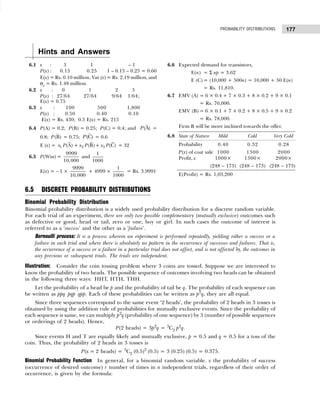
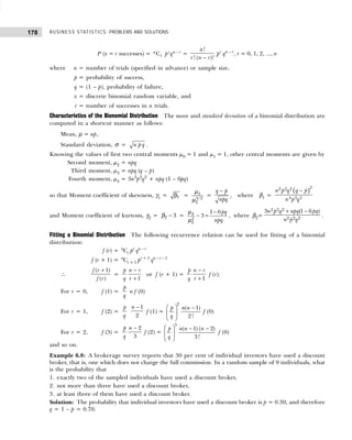
![179
PROBABILITY DISTRIBUTIONS
(a) Probability that exactly 2 of the 9 individuals have used a discount broker is given by
P(x = 2) = 9
2
C (0.30)2
(0.70)7
=
9!
(9 2)! 2!
−
(0.30)2
(0.70)7
=
9 8
2
×
× 0.09 × 0.082 = 0.2656.
(b) Probability that out of 9 randomly selected individuals not more than 3 have used a discount
broker is given by
P(x ≤ 3) = P(x =0) + P(x =1) + P(x=2) + P(x=3)
= 9
0
C (0.30)0
(0.70)9
+ 9
1
C (0.30) (0.70)8
+ 9
2
C (0.30)2
(0.70)7
+ 9
3
C (0.30)3
(0.70)6
= 0.040 + 9× 0.30×0.058 + 36×0.09×0.082 + 84×0.027×0.118
= 0.040 + 0.157 + 0.266 + 0.268 = 0.731.
(c) Probability that out of 9 randomly selected individuals, at least 3 have used a discount broker is
given by
P(x ≥ 3) = 1 – P(x < 3) = 1 – [P(x=0) + P(x=1) + P(x= 2)]
= 1 – [0.040 + 0.157 + 0.266] = 0.537.
Example 6.9: Mr Gupta applies for a personal loan of Rs. 1,50,000 from a nationalised bank to repair
his house. The loan offer informed him that over the years, bank has received about 2920 loan applications
per year and that the probability of approval was, on average, above 0.85.
(a) Mr Gupta wants to know the average and standard deviation of the number of loans approved per
year.
(b) Suppose bank actually received 2654 loan applications per year with an approval probability of 0.82.
What are the mean and standard deviation now?
Solution: (a) Assuming that approvals are independent from loan to loan, and that all loans have the
same 0.85 probability of approval. Then
Mean, µ = np = 2920 × 0.85 = 2482
Standard deviation, σ = npq = 2920 0.85 0.15
× × = 19.295.
(b) Mean, µ = np = 2654 × 0.82 = 2176.28
Standard deviation, σ = npq = 2654 0.82 0.18
× × = 19.792.
Example 6.10: Suppose 10 per cent of new scooters will require warranty service within the first months
of its sale. A scooter manufacturing company sells 1000 scooters in a month,
(a) Find the mean and standard deviation of scooters that require warranty service.
(b) Calculate the moment coefficient of skewness and kurtosis of the distribution.
Solution: Given that p = 0.10, q = 1 – p = 0.90, and n = 1000
(a) Mean, µ = np = 1000 × 0.10 = 100 scooters
Standard deviation, σ = npq = 1000 0.10 0.90
× × = 10 scootors (approx.).
(b) Moment coefficient of skewness
γ1 = 1
β =
q p
npq
−
=
0.90 – 0.10
9.48
= 0.084.
Since γ1 is more than zero, the distribution is positively skewed.
Moment coefficient of kurtosis, γ2 = β2 – 3
=
1 6 pq
npq
−
=
1 6(0.10)(0.90)
90
−
=
0.46
90
= 0.0051.
Since γ2 is positive, the distribution is platykurtic.](https://image.slidesharecdn.com/businessstatisticsproblemsandsolutions-230910073954-6d42a210/85/Business-Statistics_-Problems-and-Solutions-pdf-193-320.jpg)
![BUSINESS STATISTICS: PROBLEMS AND SOLUTIONS
180
Example 6.11: The incidence of occupational disease in an industry is such that the workers have
20 per cent chance of suffering from it. What is the probability that out of 6 workers 4 or more will come
in contact of the disease? [Lucknow Univ., MBA, 1998; Delhi Univ., MBA, 2002]
Solution: The probability of a worker suffering from the disease is p = 20/100 = 1/5. Therefore q = 1 –
p = 1 – (1/5) = 4/5.
The probability of 4 or more, that is, 4, 5, or 6 coming in contact of the disease is given by
P (x ≥ 4) = P (x = 4) + P (x = 5) + P (x = 6)
= 6
4
6
5
6
4
C C C
1
5
4
5
1
5
4
5
1
5
4 2 5 6
F
HG I
KJ F
HG I
KJ +
F
HG I
KJ F
HG I
KJ +
F
HG I
KJ
=
15 16
15625
6 4
15625
1
15625
×
+
×
+ =
1
15625
(240 + 24 + 1)
=
265
15625
= 0.01695.
Hence the probability that out of 6 workers 4 or more will come in contact of the disease is 0.01695.
Example 6.12: A multiple-choice test contains 8 questions with 3 answers to each question (of which only
one is correct). A student answers each question by rolling a balanced dice and checking the first answer
if he gets 1 or 2, the second answer if he gets 3 or 4, and the third answer if he gets 5 or 6. To get a
distinction, the student must secure at least 75 per cent correct answers. If there is no negative marking,
what is the probability that the student secures a distinction?
Solution: Probability of a correct answer, p, is one in three so that p=1/3 and probability of wrong
answer is q = 2/3.
The required probability of securing a distinction (i.e., of getting the correct answer of at least 6 of
the 8 questions) is given by
P(x ≥ 6) = P(x = 6) + P(x = 7) + P(x = 8)
=
+ +
6 2 7 8
8 8 8
6 7 8
1 2 1 2 1
C C C
3 3 3 3 3
=
6 2 2
8 8 8
6 8
7
1 2 1 2 1
3 3 3 3 3
C C C
+ +
=
× + × +
1 4 2 1
28 8
729 9 9 9
=
1
729
(12.45 + 0.178 + 0.12) = 0.0196.
Example 6.13: The screws produced by a certain machine were checked by examining the number of
defectives in a sample of 12. The following table shows the distribution of 128 samples according to the
number of defective items they contained:
(a) Fit a binomial distribution and find the expected frequencies if the chance of machine being defective
is 0.5.
(b) Find the mean and standard deviation of the fitted distribution. [Delhi Univ., MBA, 2003]
Solution: (a) The probability of a defective screw is p = 1/2, and therefore q = 1 – p = 1/2; N = 128.
Since there are 8 terms, n = 7. Thus, the probability that the defective items are 0, 1, 2, . . ., 7 is given
by
( p + q)n
= pn
+ n
C1 pn – 1
q + n
C2 pn – 2
q2
+ ⋅⋅⋅ + n
C7 pn – 7
q7
or
7
1 1
2 2
+
=
+ + + ⋅⋅⋅ +
7 6 5 2 7
7 7 7
1 2 7
1 1 1 1 1 1
C C C
2 2 2 2 2 2
No. of defectives
in a sample of 12 : 0 1 2 3 4 5 6 7
No. of samples : 7 6 19 35 30 23 7 1 = 128](https://image.slidesharecdn.com/businessstatisticsproblemsandsolutions-230910073954-6d42a210/85/Business-Statistics_-Problems-and-Solutions-pdf-194-320.jpg)
![181
PROBABILITY DISTRIBUTIONS
=
7
1
2
(1 + 7 + 21 + 35 + 35 + 21 + 7 + 1).
For obtaining the expected frequencies, multiply each term by N = 128. That is,
128
7
1 1
2 2
+
= 128 ×
1
128
(1 + 7 + 21 + 35 + 35 + 21 + 7 + 1).
Thus, the expected frequencies are
x : 0 1 2 3 4 5 6 7
f : 1 7 21 35 35 21 7 1
(b) The mean of binomial distribution is given by np and standard deviation by npq . Given that
n = 7, p = q = 1/2. Thus,
Mean= np = 7×(1/2) = 3.5,
Standard deviation = npq = × ×
7 (1/ 2) (1/ 2) = 1.75 = 1.32.
S e l f-P r a c t i c e P r o b l e m s 6B
6.9 The normal rate of infection of a certain disease in
animals is known to be 25 per cent. In an experiment
with 6 animals injected with a new vaccine it was
observed that none of the animals caught the infection.
Calculate the probability of the observed result.
6.10 Out of 320 families with 5 children each, what
percentage would be expected to have (a) 2 boys and
3 girls, (b) at least one boy? Assume equal probability
for boys and girls.
6.11 The incidence of a certain disease is such that on an
average 20 per cent of workers suffer from it. If 10
workers are selected at random, find the probability
that (a) exactly 2 workers suffer from the disease,
(b) not more than 2 workers suffer from the disease.
Calculate the probability upto fourth decimal place.
[MD Univ., M.Com., 1998]
6.12 The mean of a binomial distribution is 40 and standard
deviation 6. Calculate n, p, and q.
[Delhi Univ., MBA, 1998]
6.13 A student obtained answers with mean µ = 2.4 and
variance σ2
= 3.2 for a certain problem given to him
using binomial distribution. Comment on the result.
6.14 The probability that an evening college student will
graduate is 0.4. Determine the probability that out of
5 students (a) none, (b) one, and (c) at least one will
graduate. [Madras Univ., M.Com., 1997]
6.15 The normal rate of infection of a certain disease in
animals is known to be 25 per cent. In an experiment
with 6 animals injected with a new vaccine it was
observed that none of the animals caught infection.
Calculate the probability of the observed result.
6.16 Is there any inconsistency in the statement that the
mean of a binomial distribution is 20 and its standard
deviation is 4? If no inconsistency is found what shall
be the values of p, q, and n.
6.17 A multi-choice test consists of 8 questions with 3
answers to each question (of which only one is correct).
A student answers each question by rolling a balanced
dice and selects the first answer if he gets 1 or 2, the
second if he gets 3 or 4, and the third answer if he gets
5 or 6. To get a distribution, the student must secure
at least 75 per cent correct answers. If there is no
negative marking, what is the probability that the
student secures a distinction?
6.18 Find the probability that in a family of 5 children there
will be (a) at least one boy (b) at least one boy and one
girl (assume that the probability of a female birth is 0.5).
6.19 A famous advertising slogan claims that 4 out of 5
housewives cannot distinguish between two particular
brands of butter. If this claim is valid and 5000
housewives are tested in groups of 5, how many of
these groups will contain 0, 1, 2, 3, 4, and 5 housewives
who do not distinguish between the two products?
Assume that the capacity to distinguish between the
two brands is randomly distributed so that Bernoulli
trial conditions are satisfied.
6.20 A supposed coffee connoisseur claims that he can
distinguish between a cup of instant coffee and a cup
of percolator coffee 75 per cent of the time. It is agreed
that his claim will be accepted if he correctly identifies
at least 5 out of 6 cups. Find (a) his chance of having
the claim accepted if he is in fact only guessing and (b)
his chance of having the claim rejected when he does
have the ability he claims.](https://image.slidesharecdn.com/businessstatisticsproblemsandsolutions-230910073954-6d42a210/85/Business-Statistics_-Problems-and-Solutions-pdf-195-320.jpg)
![BUSINESS STATISTICS: PROBLEMS AND SOLUTIONS
182
Hints and Answers
6.9 Let P denote infection of the disease. Then
p = 25/100 = 1/4 and q = 3/4.
P(x = 0) = 6
C0
0 6
1 3
4 4
=
729
4096
6.10 (a) Given p = q = 1/2
P(boy = 2) = 5
C2 p2
q3
= 5
C2
2 3
1 1
2 2
=
5
16
or 31.25%
(b) P(boy ≥ 1) = 1 – 5
C0 q5
= 1 –
1
32
=
31
32
or 97 per cent.
6.11 Probability that a worker suffers from a disease, p = 1/
5 and q = 4/5.
P(x = r) = n
Cr qn – r
pr
= 10
Cr
10
1 4
5 5
r r
−
= 10
Cr
10
10
4
5
r
−
; r = 0, 1, 2, . . ., 10
(a) P(x = 2) = 10
C2
10 2
10
4
5
−
= 0.302
(b) P(x = 0) + P(x = 1) + P(x = 2)
=
10
1
5
( 10
C0 410
+ 10
C1 49
+ 10
C2 48
) = 0.678.
6.12 Given µ = np = 40 and σ = npq = 6. Squaring σ, we
get npq = 36 or 40q = 36 or q = 0.9. Then
p = 1 – q = 0.28.
Since np = 40 or n = 40/p = 40/0.1 = 400.
6.13 Given σ2
= npq = 3.2 and µ = np = 2.4. Then 2.4q =
3.2 or q =3.2/2.4 = 1.33 (inconsistent result)
6.14 Given p = 0.4 and q = 0.6
(a) P(x=no graduate) = 5
C0 (0.4) (0.6)5
= 1 × 1 × 0.0777 = 0.0777
(b) P(x = 1) = 5
C1 (0.4)1
(0.6)4
= 0.2592
(c) P(x ≥ 1) = 1 – P(x = 0) = 1 – 0.0777 = 0.9223
6.15 Probability of infection of disease = 25/100
= 0.25; q = 1 – p = 0.75.
The first term in the expansion of (q + p)n
=
6
3 1
4 4
+
is 6
C0
6
3
4
= 0.177, which is also the
required probability.
6.16 Given µ = np = 20 and σ = npq = 4 or npq
= 16 or 20q = 16 or q = 16/20 = 0.80 and then p = 1
– q = 0.20. Hence npq = 16 gives n = 16/pq = 16/(0.20
× 0.80) = 100.
6.17 Probability of correct answer, p = 1/3 and wrong
answer, q = 2/3.
Probability of securing distinction (i.e., answering at
least 6 of 8 questions correctly). That is,
P(x ≥ 6)= P(x = 6) + P(x = 7) + P(x = 8)
= 8
C6
6 2
1 2
3 3
+ 8
C7
7
1 2
3 3
+ 8
C8
8
1
3
=
6
1 4 1 2 1
28 8
3 9 3 3 9
× + × × +
=
1 129
729 9
×
= 0.019
6.18 Since p = q = 0.5,
(a) P(boy = 0) = 5
C0 (0.5)0
(0.5)5
= 0.031
P(at least one boy) = 1 – 0.031 = 0.969
(b) P(at least 1B and 1G) = 5
C1 (0.5)1
(0.5)4
+ 5
C2 (0.5)2
(0.5)3
+5
C3 (0.5)3
(0.5)2
+ 5
C4 (0.5)4
(0.5)
=
5 10 10 5
32 32 32 32
+ + + =
30
32
6.19 p = probability that 4 out of 5 cannot distinguish
between two brands = 4/5 = 0.8
so that q = 1 – p = 1/5 = 0.2
Expected distribution containing 0, 1, . . ., 5 housewives
who do not distinguish between two brands
= 5
C0 (0.2)5
+ 5
C1 (0.8) (0.2)4
+ 5
C2 (0.8)2
(0.2)3
+ 5
C3 (0.8)3
(0.2)2
+ 5
C4 (0.8)4
(0.2)1
+ 5
C5 (0.8)5
Thus, required number in each group would be
5000 (0.2)5
; 5000 5
C1 (0.8) (0.2)4
;
5000 5
C2 (0.8)2
(0.2)3
; 5000 5
C3 (0.8)3
(0.2)2
;
5000 5
C4 (0.8)4
(0.2); 5000 (0.8)5
6.20 Given p = probability that he is capable of making
a distinction = 0.75; q = 1 – p = 0.25
(a) P(x < 5) = 1 – P(x ≥ 5)
= 1 – [6
C5 (0.75)5
(0.25) + 6
C6 (0.75)6
]
= 1 – 0.534 = 0.466
(b) P(x ≥ 5) = 0.534](https://image.slidesharecdn.com/businessstatisticsproblemsandsolutions-230910073954-6d42a210/85/Business-Statistics_-Problems-and-Solutions-pdf-196-320.jpg)
![183
PROBABILITY DISTRIBUTIONS
6.6 POISSON PROBABILITY DISTRIBUTION
The Poisson process measures the number of occurrences of a particular outcome of a discrete random variable
in a predetermined time interval, space, or volume, for which an average number of occurrences of the outcome are
known or can be determined. In the Poisson process, the random variable values need counting.
The Poisson probability distribution provides a simple, easy-to-compute and accurate approximation
to a binomial distribution when the probability of success, p, is very small and n is large, so that µ = np is
small, preferably np > 7. It is often called the law of improbable events meaning that the probability, p, of
a particular event’s happening is very small.
Poisson probability function If the probability, p, of occurrence of an outcome of interest (i.e., success) in
each trial is very small, but the number of independent trials n is sufficiently large, then the average
number of times that an event occurs in a certain period of time or space, λ = np, is also small. Under
these conditions the binomial probability function
P(x = r) = n
Cr pr
qn – r
=
( 1)( 2) . . . ( 1)
!
n n n n r
r
− − − +
pr
qn – r
=
1 2 1
1 1 . . . 1 1 ;
!
n r
r
r
n n n r n
−
−
− − − −
λ λ
np = λ or p = λ/n
tends to
!
r
e
r
−λ
λ
for a fixed r. Thus, the Poisson probability distribution that approximates the binomial
distribution is defined by the following probability function:
P(x = r) =
!
r e
r
− λ
λ
, r = 0, 1, 2, . . .
where e = 2.7183.
Characteristics of Poisson Distribution
• The arithmetic mean, µ = E (x), of Poisson distribution is given by
µ = P( ) ,
!
x
e
x x x
x
−
=
∑ ∑
λλ
x = 1, 2, 3, . . . and x P(x) = 0 for x = 0
=
3
2 . . . . . .
2! ( 1)!
r
e e
e e
x
− −
− −
+ + + + +
−
λ λ
λ λ λ λ
λ λ
=
2 1
. ..
. ..
1
2! ( 1)!
r
e
x
−
−λ
+ + + + +
−
λ λ
λ λ = e e
−λ λ
λ = λ.
Thus, the mean of the distribution is µ = λ = np.
• The variance σ 2
of Poisson distribution is given by
σ2
= E(x2
) – [E(x)]2
= E(x2
) – λ2
= 2 2
!
x
e
x
x
−
−
∑
λλ
λ = 2
( 1)
!
x
x x x
e
x
− − +
−
∑
λ λ λ
=
2 1
2 2
( 2)! ( 1)!
x x
e e
x x
− −
− −
+ −
− −
∑ ∑
λ λ
λ λ
λ λ λ
= λ2
e–λ
eλ
+ λ e–λ
eλ
– λ2
= λ2
+ λ – λ2
= λ.
Thus, the variance of the distribution is σ 2
= λ = np.
µ2 = µ3 = λ and µ4 = λ + 3λ2](https://image.slidesharecdn.com/businessstatisticsproblemsandsolutions-230910073954-6d42a210/85/Business-Statistics_-Problems-and-Solutions-pdf-197-320.jpg)
![BUSINESS STATISTICS: PROBLEMS AND SOLUTIONS
184
so that moment coefficient of skewness, γ1 = 1
β =
1
λ
and moment coefficient of kurtosis, γ2 = β2 – 3 =
1
λ
.
Fitting a Poisson Distribution A Poisson distribution can be fitted to the observed values in the data set by
simply obtaining values of λ and calculating the probability of zero occurrence. Other probabilities can
be calculated by the recurrence relation as follows:
f (r) =
!
r
e
r
− λ λ
f (r + 1) =
1
( 1) !
r
e
r
− +
+
λ λ
or
( 1)
( )
f x
f r
+
=
1
r +
λ
or f (r + 1) =
( 1)
r +
λ
f (r) ; r = 0, 1, 2, ...
Thus, for r = 0, f (1) = λ f (0),
for r = 1, f (2) =
2
λ
f (1) =
2
2
λ
f (0)
and so on, where f (0) = e–λ
.
After obtaining the probability for each of the random variable values, multiply each of them by N
(total frequency) to get the expected frequency for the respective values.
Example 6.14: What probability model is appropriate to describe a situation where 100 misprints are
distributed randomly throughout the 100 pages of a book? For this model, what is the probability that a
page observed at random will contain at least 3 misprints?
Solution: Since 100 misprints are distributed randomly throughout the 100 pages of a book, on an
average there is only one mistake on a page. This means, the probability of there being a misprint, p =
1/100, is very small and the number of words, n, in 100 pages are very large. Hence, Poisson distribution
is best suited in this case.
Average number of misprints in one page, λ = np = 100×(1/100) = 1. Therefore, e–λ
= e–1
= 0.3679.
Probability of at least 3 misprints in a page is
P(x ≥ 3) = 1 – P (x < 3) = 1 – {P (x = 0)+P (x = 1)+P (x = 2)}
= 1 – [e–λ
+ λ e–λ
+
1
2!
λ2
e–λ
] = 1 –
1
1 1
2!
e
e e
−
− −
+ +
= 1 – 2.5 e –1
= 1 – 2.5 (0.3679) = 0.0802.
Example 6.15: A new automated production process has had an average of 1.5 breakdowns per day.
Because of the cost associated with a breakdown, management is concerned about the possibility of having
three or more breakdowns during a day. Assume that breakdowns occur randomly, that the probability of
a breakdown is the same for any two time intervals of equal length, and that breakdowns in one period are
independent of breakdowns in other periods. What is the probability of having three or more breakdowns
during a day? [HP Univ., MBA, 1995; Kumaon Univ., 1998]
Solution: Given that λ = np = 1.5 breakdowns per day. Thus, probability of having three or more
breakdowns during a day is given by
P(x ≥
≥
≥
≥
≥ 3) = 1 – P(x < 3) = 1 – [P(x= 0) + P(x=1) + P(x=2)]
= 1 –
2
0 –
0! 1! 2!
e e
e − −
+ +
λ λ
λ λ λ
λ](https://image.slidesharecdn.com/businessstatisticsproblemsandsolutions-230910073954-6d42a210/85/Business-Statistics_-Problems-and-Solutions-pdf-198-320.jpg)
![185
PROBABILITY DISTRIBUTIONS
= 1 – e–λ 2
1
1
2
+ +
λ λ = 1 – 0.2231 2
1
1 1.5 (1.5)
2
+ +
= 1 – 0.2231 (3.625) = 1 – 0.8088 = 0.1912.
Example 6.16: Suppose a life insurance company insures the lives of 5000 persons aged 42. If studies
show the probability that any 42-year old person will die in a given year to be 0.001, find the probability
that the company will have to pay at least two claims during a given year.
Solution: Given that n = 5000, p = 0.001, so λ = np = 5000×0.001 = 5. Thus, the probability that the
company will have to pay at least 2 claims during a given year is given by
P(x ≥
≥
≥
≥
≥ 2) = 1 – P(x < 2) = 1 – [P(x = 0) + P(x = 1)]
= 1 – [e–λ
+ λe–λ
] = 1 – [e–5
+ 5e–5
] = 1 – 6e–5
= 1 – 6×0.0067 = 0.9598.
Example 6.17: A manufacturer who produces medicine bottles finds that 0.1 per cent of the bottles are
defective. The bottles are packed in boxes containing 500 bottles. A drug manufacturer buys 100 boxes
from the producer of bottles. Using Poisson distribution, find how many boxes will contain
(a) no defectives and (b) at least two defectives [Delhi Univ., MBA, 1996, 2001]
Solution: Given that p = 1 per cent = 0.001, n = 500, λ = np = 500×0.001 = 0.5.
(a) P[x = 0] = e– λ
= e– 0.5
= 0.6065.
Therefore, the required number of boxes are 0.6065×100 = 61 (approx.)
(b) P(x > 2) = 1 – P(x ≤ 1) = 1 – [P(x = 0) + P(x = 1)]
= 1 – [eλ
+ λ e– λ
] = 1 – [0.6065 + 0.5(0.6065)]
= 1 – 0.6065 (1.5) = 1 – 0.90975 = 0.09025.
Therefore, the required number of boxes are 100×0.09025 = 10 (approx.)
Example 6.18: The following table gives the number of days in a 50-day period during which automobile
accidents occurred in a city:
No. of accidents : 0 1 2 3 4
No. of days : 21 18 7 3 1
Fit a Poisson distribution to the data. [Sukhadia Univ., MBA,1992; Kumaon Univ., MBA, 2000]
Solution: Calculations for fitting of Poisson distribution are shown in Table 6.4.
Thus, (or )
x λ =
f x
n
Σ
=
45
50
= 0.9
and P(x=0) = e–λ
= e–0.9
= 0.4066
P(x=1) = λ P(x=0)= 0.9(0.4066)=0.3659
P(x=2) =
2
λ
P(x=1)=
0.9
2
(0.3659)=0.1647
Table 6.4 Calculations for Poisson Distribution
Number of Accidents (x) Number of Days ( f) f x
0 21 0
1 18 18
2 7 14
3 3 09
4 1 04
n = 50 Σ fx = 45](https://image.slidesharecdn.com/businessstatisticsproblemsandsolutions-230910073954-6d42a210/85/Business-Statistics_-Problems-and-Solutions-pdf-199-320.jpg)
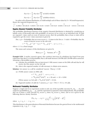
![187
PROBABILITY DISTRIBUTIONS
Example 6.20: In a factory producing certain items, 30 per cent of the items produced have no defect,
40 per cent have one defect, and 30 per cent have two defects. A random sample of 8 items is taken from
a day’s output. Find the probability that it will contain 2 items with no defect, 3 items with one defect, and
3 items with two defects.
Solution: We know from the data that n = 8, p1 = 0.30, p2 = 0.40, and p3 = 0.30; x1 = 2, x2 = 3, and
x3 = 3. Thus, the required probability is given by
P(x1=2, x2=3, x3=3) =
8!
2! 3! 3!
[(0.30)2
(0.40)2
(0.30)3
] = 0.0871.
Hypergeometric Probability Distribution
Hypergeometric probability distribution is similar to binomial distribution where probability of success
may be different from trial to trial. When sampling is done without replacement from a finite population,
the Bernoulli process does not apply because there is a systematic change in the probability of success in
the reduced size of population.
Let N be the size of population and out of N, m be the total number of elements having a certain
characteristic (called success) and the remaining N – m do not have it, such that p + q = 1. Suppose a
sample of size n is drawn at random without replacement. Then in a random sample of size n, the
probability of exactly r sucesses when values of r depend on N, p, and n is given by
P(x = r) = N
C C
C
N m
m
r n r
n
−
−
; r = 0, 1, 2, . . ., n ; and 0 ≤ r ≤ m.
This probability mass function is called hypergeometric probability distribution.
The mean and variance of a hypergoemetric distribution are
Mean = n
m
N
and Variance =
1
m N m N n
n
N N N
− −
−
.
Example 6.21: Suppose the HRD manager randomly selects 3 individuals from a group of 10 employees
for a special assignment. Assuming that 4 of the employees were assigned to a similar assignment previously,
determine the probability that exactly two of the three employees have had previous experience.
Solution: We know from the data that N = 10, n = 3, r = 2, m = 4, and N – m = 6. Thus the required
probability is given by
P(x = r | N, m, N – m) =
N
N
C C
C
m
m
r n r
n
−
−
=
4
2 3
3
C C
C
10 4
2
10
−
−
=
4 6
2 1
10
3
C C
C
=
4! 6!
2! 2! 1!5!
10!
3!7!
=
36
120
= 0.30.
Example 6.22: Suppose a particular industrial product is shipped in lots of 20. To determine whether
an item is defective a sample of 5 items from each lot is drawn. A lot is rejected if more than one defective
item is observed. (If the lot is rejected, each item in the lot is then tested). If a lot contains four defectives,
what is the probability that it will be accepted?
Solution: Let r be the number of defectives in the sample size n = 5. Given that N = 20, m = 4, and
N – m = 16. Then
P(accept the lot) = P(x ≤ 1) = P(x = 0) + P(x = 1)
=
4 16 4 16
0 5 1 4
20 20
5 5
C C C C
C C
× ×
+ =
4! 16!
4! 16!
1!3! 4!12!
0!4! 5!11!
20! 20!
5!15! 5!15!
×
×
+
=
91 455
323 969
+ = 0.2817 + 0.4696 = 0.7513.](https://image.slidesharecdn.com/businessstatisticsproblemsandsolutions-230910073954-6d42a210/85/Business-Statistics_-Problems-and-Solutions-pdf-201-320.jpg)
![BUSINESS STATISTICS: PROBLEMS AND SOLUTIONS
188
S e l f-P r a c t i c e P r o b l e m s 6C
6.21 The following table shows the number of customers
returning the products in a marketing territory. The
data are for 100 stores:
No. of returns : 0 1 2 3 4 5 6
No. of stores : 4 14 23 23 18 9 9
Fit a Poisson distribution. [Lucknow Univ., MBA, 1997]
6.22 In a certain factory manufacturing razor blades, there
is a small chance of 1/150 for any blade to be defective.
The blades are placed in packets, each containing 10
blades. Using the Poisson distribution, calculate the
approximate number of packets containing not more
than 2 defective blades in a consignment of 10,000
packets.
6.23 In a town 10 accidents took place in a span of 50 days.
Assuming that the number of accidents per day follows
the Poisson distribution, find the probability that there
will be three or more accidents in a day.
[Coimbatore Univ., MBA, 1997]
6.24 The distribution of typing mistakes committed by a
typist is given below. Assuming a Poisson distribution,
find out the expected frequencies:
No. of mistakes
per page : 0 1 2 3 4 5
No. of pages : 142 156 69 27 5 1
[Rohilkhand Univ., MBA, 1998]
6.25 Find the probability that at most 5 defective bolts will
be found in a box of 200 bolts if it is known that 2 per
cent of such bolts are expected to be defective [you
may take the distribution to be Poisson; e–4 = 0.0183].
6.26 It is given that 30 per cent of electric bulbs
manufactured by a company are defective. Find the
probability that a sample of 100 bulbs will contain
(a) no defective and (b) exactly one defective.
6.27 One-fifth per cent of the blades produced by a blade
manufacturing factory turn out to be defective. The
blades are supplied in packets of 10. Use Poisson
distribution to calculate the approximate number of
packets containing no defective, one defective, and
two defective blades respectively in a consignment of
1,00,000 packets. [Delhi Univ., MBA, 1999, 2003]
6.28 A factory produces blades in packets of 10. The
probability of a blade to be defective is 0.2 per cent.
Find the number of packets having two defective blades
in a consignment of 10,000 packets.
6.29 When a first proof of 200 pages of an encyclopaedia
of 5000 pages was read, the distribution of printing
mistakes was found to be as shown in the first and
second columns of the table below. Fit a Poisson
distribution to the frequency distribution of printing
mistakes. Estimate the total cost of correcting the
whole encyclopaedia by using the information given
in the first and third columns of the table below:
Misprints Frequency Cost of Detection and
on a Page Correction Per Page (Rs.)
0 113 1.00
1 162 2.50
2 120 1.50
3 113 3.00
4 111 3.50
5 111 4.00
[MD Univ., MBA, 1998]
6.30 In a certain factory manufacturing razor blades, there
is small chance 1/50 for any blade to be defective. The
blades are placed in packets, each containing 10 blades.
Using an appropriate probability distribution, calculate
the approximate number of packets containing not
more than 2 defective blades in a consignment of
10,000 packets.
6.31 Suppose that a manufactured product has 2 defects
per unit of product inspected. Using Poisson
distribution, calculate the probabilities of finding a
product without any defect, 3 defects, and 4 defects.
(Given e–2
= 0.135) [Madurai Univ., M.Com., 1999]
6.32 A distributor received a shipment of 12 TV sets.
Shortly after this shipment was received, the
manufacturer informed that he had inadvertently
shipped 3 defective sets. The distributor decided to
test 4 sets randomly selected out of 12 sets received.
(a) What is the probability that neither of the 4
sets tested was defective?
(b) What is the mean and variance of defective sets.
6.33 Suppose a population contains 10 elements, 6 of which
are defective. A sample of 3 elements is selected. What
is the probability that exactly 2 are defective?
6.34 A transport company has a fleet of 15 trucks, used
mainly to deliver fruits to wholesale market. Suppose
6 of the 15 trucks have brake problems. Five trucks
were selected at random to be tested. What is the
probability that 2 of those tested trucks have defective
brakes?
6.35 A company has five applicants for two positions:
two women and three men. Suppose that the five
applicants are equally qualified and that no preference
is given for choosing either gender. If r equal the
number of women chosen to fill the two positions,
then what is the probability distribution of r. Also,
determine the mean and variance of this distribution.](https://image.slidesharecdn.com/businessstatisticsproblemsandsolutions-230910073954-6d42a210/85/Business-Statistics_-Problems-and-Solutions-pdf-202-320.jpg)
![189
PROBABILITY DISTRIBUTIONS
Hints and Answers
6.21 Fitting of Poisson distribution
x : 0 01 02 03 04 05 06
f : 4 1 4 2 3 2 3 1 8 09 09 = 100
fx : 0 1 4 4 6 6 9 7 2 4 5 5 4 = 300
∴ λ = 300/100 = 3. Then
NP(x = 0) = 100 e– λ
= 100(2.7183)– 3
= 5;
P(x = 1) = λ NP(0) = 15
P(x = 2) = NP(x = 1)
2
λ
= 22.5;
P(x = 3) = NP(x = 2)
3
λ
= 22.5
P(x = 4) = NP(x = 3)
4
λ
= 16.9;
P(x = 5) = NP(x = 4)
5
λ
= 10.1
P(x = 6) = NP(x = 5)
6
λ
= 5.1
6.22 Given that N = 10,000, p = 1/50, n = 10, λ = np
= 10 × (1/50) = 0.2
P(x = 0) = e– λ
= e– 0.2
= 0.8187 (from the table)
NP(x = 0) = 0.8187 × 10,000 = 8187
NP(x = 1) = NP(x = 0) × λ = 8187 × 0.2 = 1637.4
NP(x = 2) = NP(x = 1) × λ/2
= 1637.4 × (0.2/2) = 163.74
The approximate number of packets containing not
more than 2 defective blades in a consignment of
10,000 packets is 10,000 – (8187+163.74+163.74)
= (10,000 – 9988.14) = 11.86 or 12.
6.23 The average number of accidents per day
= 10/50 = 0.2
P(x ≥ 3 accidents) = 1 – P(2 or less accidents)
= 1 – [P(0) + P(1) + P(2)]
= –
2
2 2 0.2 0.2
2
2
e
e e
−
− −
× ×
+ +
= 1 – e– 2
[1 + 0.2 + 0.02] = 1 – 0.8187× 1.22
(From table of e– λ
)
= 1 – 0.998 = 0.002
6.24 λ = Σ fx / N = 400/400 = 1,
P(x = 0) = e–λ
= 0.3679
NP(x = 0) = 147.16
NP(x = 1) = NP(x = 0)λ = 147.16
NP(x = 2)= NP (x = 1)
2
λ
= 73.58
NP(x = 3)= NP(x = 2)
3
λ
= 24.53
NP(x = 4)= NP(x = 3)
4
λ
= 6.13
NP(x = 5)= NP (x = 4)
5
λ
= 1.23
Expected frequencies as per the distribution are
No. of mistakes
per page : 0 1 2 3 4 5
No. of pages : 147 147 74 25 6 1
6.25 p(defective bolt) = 2% = 0.02. Given n = 200, so
λ = np = 200 × 0.02 = 4
P(0) =
0
0!
e− λ
λ
= e– 4
= 0.0183
P(x ≤ 5) = P(x = 0) + P(x = 1) + P(x = 2)
+ P(x = 3) + P(x = 4) + P(x = 5)
= e−
+ + + + +
F
HG
I
KJ
4
2 3 4 5
1 4
4
2
4
3
4
4
5
5
! ! ! !
= 0.0183 × (643/15) = 0.7844.
6.26 λ = np = 100 × 0.30 = 3
P(x = 0)= e–λ
= e–3
= 0.05;
P(x = 1) = λP(x = 0) = 3 × 0.03= 0.15
6.27 Given n = 10, p = 1/500, λ = np = 10/500
= 0.02
(i) P(x = 0) = e–λ
= e–0.02
= 0.9802
NP(x = 0) = 1,00,000 × 0.9802
= 98020 packets
(ii) P(x = 1) = λP(x = 0)
= λ e–λ
= 0.02 × 0.9802
= 0.019604
NP(x = 1) = 1,00,000 × 0.019604
= 1960 packets
(iii) P(x = 2) =
2
2
λ
P(x = 0)
=
( )2
0.02
2
× 0.9802
= 0.00019604
NP(x = 2) = 1,00,000 × 0.00019604
= 19.60 ≅ 20 packets
6.28 Given n = 10, p = 0.002, λ = np = 10 × 0.002 = 0.02.
P(x = 2) =
2
2!
e−λ λ
=
0.02 2
(0.02)
2!
e−
= 0.000196](https://image.slidesharecdn.com/businessstatisticsproblemsandsolutions-230910073954-6d42a210/85/Business-Statistics_-Problems-and-Solutions-pdf-203-320.jpg)
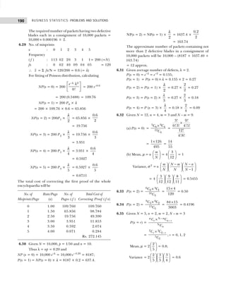
![191
PROBABILITY DISTRIBUTIONS
6.7 CONTINUOUS PROBABILITY DISTRIBUTIONS
Nature seems to follows a predictable pattern for many kinds of measurments. Most numerical values of
a random variable are spread arround the centre, and greater the distance a numerical value has from the
centre, the fewer numerical values have that specific value. A frequency distribution of values of random
variable observed in nature which follows this pattern is approximately bell shaped. A special case of
distribution of measurements is called a normal curve (or distribution).
Normal Probability Distribution Function
The formula that generates normal probability distribution is as follows:
f (x) =
2
( 1/ 2)[( )/ ]
1
2
x
e − −
π
µ σ
σ
, –∞ < x < ∞
where π = constant 3.1416,
e = constant 2.7183,
µ = mean of the normal distribution,
σ = standard of normal distribution.
The f (x) values represent the relative frequencies (height of the curve) within which values of random
variable x occur. The distribution is symmetric about its mean µ that locates at the centre.
Since the total area under the normal probability distribution is equal to 1, the symmetry implies that the
area on either side of µ is 50 per cent or 0.5. The shape of the distribution is determined by µ and σ values.
Characteristics of the Normal Probability Distribution There is a family of normal distributions. Each normal
distribution may have a different mean µ or standard deviation σ. A unique normal distribution may be
defined by assigning specific values to the mean µ and standard deviation σ in the normal probability
density function. Large value of σ reduce the height of the curve and increase the spread; small values of
σ increase the height of the curve and reduce the spread.
When the normal random variable x is expressed in terms of standard units, that is, z = (x – µ)/r, the
normal probability density function is expressed as
f(x) =
2
1/2
1
2
z
e−
π
.
Standard Normal Probability Distribution: The standardized normal random variable, z (also called z–statistic, z–
score or normal variate), is defined as
z =
x − µ
σ
or x = µ + zσ.
A z–score measures the number of standard deviations that a value of the random variable x fall from
the mean.
Figure6.4 StandardNormalDistribution](https://image.slidesharecdn.com/businessstatisticsproblemsandsolutions-230910073954-6d42a210/85/Business-Statistics_-Problems-and-Solutions-pdf-205-320.jpg)
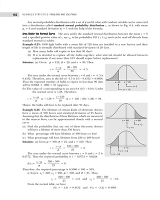
![193
PROBABILITY DISTRIBUTIONS
Thus the required probability is
P(z = –3.2) – P(z = –1.6) = 0.4903 – 0.4452 = 0.0541.
Hence the required percentage = 0.0541 × 100 = 5.41 per cent.
Example 6.25: In a certain examination, the percentage of passes and distinctions were 46 and 9
respectively. Estimate the average marks obtained by the candidates, the minimum pass and distinction
marks being 40 and 75 respectively (assume the distribution of marks to be normal).
Also determine what would have been the minimum qualifying marks for admission to a re-examination
of the failed candidates, had it been desired that the best 25 per cent of them should be given another
opportunity of being examined.
Solution: (a) Let µ be the mean and σ be the standard deviation of the normal distribution. The area to
the right of the ordinate at x = 40 is 0.46 and hence the area between the mean and the ordinate at x =
40 is 0.04.
Now from the normal table, corresponding to 0.04, the standard normal variate,
z = 0.1. Therefore, we have
40 − µ
σ
= 0.1 or 40 – µ = 0.1σ.
Similarly,
75 − µ
σ
= 1.34 or 75 – µ = 1.34 σ.
Solving these equations, we get σ = 28.23 and µ = 37.18 or 37.
(b) Let us assume that x1 is the minimum qualifying marks for re-examination of the failed candidates.
The area to the right of x = 40 is 46 per cent. Thus the percentage
of students failing = 54 and this is the area to the left of 40. We want
that the best 25 per cent of these failed candidates should be given a
chance to reappear. Suppose this area is equal to the shaded area in
the diagram. This area is 25 per cent of 54 = 13.5 per cent = 0.1350.
The area between mean and ordinate at x1 = – (0.1350 – 0.04)
= –0.0950 (negative sign is included because the area lies to the left
of the mean ordinates).
Corresponding to this area, the standard normal variate z = –0.0378. Thus, we write
1
x − µ
σ
= – 0.0378
x1 = µ – 0.0378 σ = 37.2 – (0.0378 × 28.23)
= 37.2 – 1.067 = 36.133 or 36 (approx.)
Example 6.26: In a normal distribution, 31 per cent of the items
are under 45 and 8 per cent are over 64. Find the mean and standard
deviation of the distribution. [Delhi Univ., MBA, 1999]
Solution: Since 31 per cent of the items are under 45, the left of the
ordinate at x = 45 is 0.31, and obviously the area to the right of the
ordinate up to the mean is (0.5 – 0.31) = 0.19. The value of z
corresponding to this area is 0.5. Hence,](https://image.slidesharecdn.com/businessstatisticsproblemsandsolutions-230910073954-6d42a210/85/Business-Statistics_-Problems-and-Solutions-pdf-207-320.jpg)
![BUSINESS STATISTICS: PROBLEMS AND SOLUTIONS
194
z =
45 − µ
σ
= – 0.5 or – µ + 0.5σ = –45.
As 8 per cent of the items are above 64, area to the right of the ordinate at 64 is 0.08. Area to the left
of the ordinate at x = 64 up to mean ordinate is (0.5 – 0.08) = 0.42 and the value of z corresponding to
this area is 1.4. Hence
z =
64 − µ
σ
= 1.4 or – µ – 1.4σ = –64.
From these two equations, we get 1.9 σ = 19 or σ = 10. Putting σ = 10 in the first equation, we get
µ – 0.5 × 10 = 45 or µ = 50.
Thus, mean of the distribution is 50 and standard deviation is 10.
Example 6.27: The income of a group of 10,000 persons was found
to be normally distributed with mean Rs. 1750 per month and
standard deviation Rs. 50. Show that of this group 95% had income
exceeding Rs. 1668 and only 5 per cent had income exceeding
Rs. 1832. What was the lowest income among the richest 100?
[Delhi Univ., MBA, 1997]
Solution: (a) Given that x = 1668, µ = 1750, and σ = 50. Therefore,
the standard normal variate corresponding to x = 1668 is
z =
x − µ
σ
=
1668 1750
50
−
= –1.64.
The area to the right of the ordinate at z = –1.64 (or x = 1668)
is (0.4495 + 0.5000) = 0.9495 (because z = –1.64 to its right covers
95 per cent area).
The expected number of persons getting above Rs. 1668 are
10,000 × 0.9495 = 9495. This is about 95 per cent of the total of
10,000 persons.
(b) The standard normal variate corresponding to x = 1832 is
z =
1832 1750
50
−
= 1.64.
The area to the right of ordinate at z = 1.64 is 0.5000 – 0.4495
= 0.0505.
The expected number of persons getting above Rs. 1832 is 10,000 × 0.0505 = 505. This is about
5 per cent of the total of 10,000 persons. Thus, probability of getting richest 100 out of 10,000 is 100/
10,000 = 0.01.
The standard normal variate having 0.01 area to its right is z = 2.33. Hence
2.33 =
1750
50
x −
x = 2.33 × 50 + 1750 = Rs. 1866 approx.
This implies that the lowest among the richest 100 is getting Rs. 1866 per month.
Example 6.28: A wholesale distributor of fertilizer products finds
that the annual demand for one type of fertilizer is normally
distributed with a mean of 120 tonnes and standard deviation of 16
tonnes. If he orders only once a year, what quantity should be ordered
to ensure that there is only a 5 per cent chance of running short?
[Delhi Univ., MBA, 1998, 2000]
Solution: Let x be the annual demand (in tonnes) for one type of
fertilizer. Therefore,](https://image.slidesharecdn.com/businessstatisticsproblemsandsolutions-230910073954-6d42a210/85/Business-Statistics_-Problems-and-Solutions-pdf-208-320.jpg)
![195
PROBABILITY DISTRIBUTIONS
z =
120
16
x −
.
The desired area of 5 per cent is shown in the figure. Since the area between the mean and the given
value of x is 0.45, from the normal table this area of 0.45 corresponds to z = 1.64.
Substituting this value of z = 1.64 in standard normal variate, we get
1.64 =
120
16
x −
or x = 120 + (1.64) (16) = 146.24 tonnes.
If it is necessary to order in whole units, then the wholesale distributor should order 147 tonnes.
Example 6.29: Assume that the test scores from a college admissions test are normally distributed with a
mean of 450 and a standard deviation of 100.
(a) What percentage of people taking the test score are between 400 and 500?
(b) Suppose someone received a score of 630. What percentage of the people taking the test score better?
What percentage score worse?
(c) If a particular university will not admit any one scoring below
480, what percentage of the persons taking the test would be
acceptable to the university? [Delhi Univ. MBA, 2003]
Solution: (a) Given µ = 450 and σ = 100. Let x be the test score.
Then
z1 =
x − µ
σ
=
500 – 450
100
= 0.5
and z2 =
x − µ
σ
=
400 – 450
100
= – 0.5.
The area under the normal curve between z = 0 and z = 0.5 is 0.1915.
The required probability that the score falls between 400 and 500 is
P(400 ≤ x ≤ 500) = P(–0.5 ≤ z ≤ 0.5) = 0.1915 + 0.1915 = 0.3830.
So the percentage of the people taking the test score between 400 and 500 is 38.30 per cent.
(b) Given x = 630, µ = 450, and σ = 100. Thus,
z =
x − µ
σ
=
630 – 450
100
= 1.8.
The area under the normal curve between z = 0 and z = 1.8 is
0.4641.
The probability that people taking the test score better is given
by
P(x ≥ 630) = P(z ≥ 1.8) = 0.5000 + 0.4641 = 0.9640.
That is, 96.40 per cent people score better.
The probability that people taking the test score worse is given
by
P(x ≤ 630) = P(z ≤ 1.8) = 0.5000 – 0.4641 = 0.0.0359.
That is, 3.59 per cent people score worse.
(c) Given x = 480, µ = 450, and σ = 100. Thus
z =
x − µ
σ
=
480 – 450
100
= 0.30.](https://image.slidesharecdn.com/businessstatisticsproblemsandsolutions-230910073954-6d42a210/85/Business-Statistics_-Problems-and-Solutions-pdf-209-320.jpg)
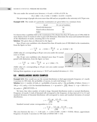
![197
PROBABILITY DISTRIBUTIONS
Example 6.32: If on an average 8 ships out of 10 arrive safely at a port, find the mean and standard
deviation of the number of ships arriving safely out of a total of 1600 ships.
[Kurukshetra Univ., MBA, 2004]
Solution: Probability of safe arrival, p = 8/10 = 0.8 and q= 1 – p =1 – 0.8 =0.2.
Mean number of ships returning safely: m(= np) = 1600 ×0.8 = 1280.
Standard deviation, σ = npq = × ×
1600 0.8 0.2 =16.
Hence the mean and standard deviation of ships returning safely is respectively 1280 and 16.
Example 6.33: The following table shows the number of customers returning the products in a marketing
territory. The data is for 100 stores;
No. of returns : 0 1 2 3 4 5 6
Frequency : 4 14 23 23 18 9 9
Fit a Poission distribution. [Lucknow Univ., MBA, 2006]
Solution: Calculations required to fit a Poisson distribution are shown below:
x f f x
0 4 0
1 14 14
2 23 46
3 23 69
4 18 72
5 9 45
6 9 54
N = 100 300
x =
Σ 300
= = 3
100
f x
n
.
Hence, the mean of Poisson distribution, that is, m = 3.
P(x=0)= e–m
= (2.7183)–3
= 0.0498
n P (x=0)= 10×0.0498 = 0.498
n P(x=1)= n P(x = 0) × m = 10×0.498 × 3 = 14.94
n P(x=2)= = × ×
3
( 1) =14.94 = 22.41
2 2
m
n P x
n P(x=3)= = × ×
3
( 2) = 22.41 = 22.41
3 3
m
n P x
n P(x=4)= = × ×
3
( 3) = 22.41 =16.80
4 4
m
n P x
n P(x=5)= = × ×
3
( 4) =16.80 =10.08
5 5
m
n P x
n P(x=6)= = × ×
3
( 5) =10.08 =5.04.
6 6
m
n P x
Example 6.34: A multiple-choice test consists of 8 questions with 3 answers to each question (of which
only one is correct). A student answers each question by rolling a balanced dice and checking the first
answer if he gets 1 or 2, the second answer if he gets 3 or 4, and the third answer if he gets 5 or 6. To get
a distinction, the student msut secure at least 75% correct answers. If there is no negative marking, what
is the probability that the student secures a distinction? [Delhi Univ., B.A.(Eco. H), 2002]
Solution: Probability of getting a correct answer to a question: p =1/3 and therefore q =2/3.](https://image.slidesharecdn.com/businessstatisticsproblemsandsolutions-230910073954-6d42a210/85/Business-Statistics_-Problems-and-Solutions-pdf-211-320.jpg)
![BUSINESS STATISTICS: PROBLEMS AND SOLUTIONS
198
Now the probability of getting correctly r answers in 8 questions test is given by
P (x=r) = 8
C1 pr
q8– r
; r = 0, 1, 2,...8.
The required probability ‘p’ of securing a distinction (i.e., of getting correct answers of at least 6 of the 8
questions) is given by
P(x = r) = P(6) + P(7) + P(8)
=
1
+ +
6 2 7 8
8 8 8
6 7 8
1 2 1 2
3 3 3 3 3
C C C
=
× + × × +
1 4 1 2 1
27 8
36 9 3 3 9
= + +
1
(12 0.1778 0.111)
729
= =
13.889
0.019
729
Example 6.35: In a town, 10 accidents took place in a span of 50 days. Assuming that the number of
accidents per day follows the Possion distribution, find the probability that there will be three or more
accidents in a day. [Coimbatore Univ., MBA, 2005]
Solution: The average number of accidents per day are 10/50=0.2. Thus,
P (3 or more accidents) = 1 – P (2 or less accidents)
= 1 – [P(0) + P(1) + P(2)]
=
−
− −
×
− + × +
2 2
2 2 (0.2)
1 0.2
2!
e
e e
= 1 – e–2
[1 + 0.2 + 0.02] = 1 – e–2
×1.22
= 1 – 0.8187× 1.22 = 1–0.999= 0.001.
Example 6.36: When the first proof of 200 pages of an encyclopedia of 5000 pages was read, the distribution
of printing mistakes was found to be as shown in the first and second columns of the table below. Fit a
Poisson distribution to the frequency distribution of printing mistakes. Estimate the total cost of correcting
the whole encyclopaedia by using the information given in the first and third columns of the table below:
No. of Misprints Frequency Cost of Detection and
per page Correction per Page (Rs.)
0 113 1.00
1 62 2.50
2 20 1.50
3 3 3.00
4 1 3.50
5 1 4.00
[MD Univ., MBA, 2005]
Solution: Fitting Poisson distribution as follows:
No. of Mistakes Frequency
per page (x) (f) f x
0 113 0
1 62 62
2 20 40
3 3 9
4 1 4
5 1 5
200 120](https://image.slidesharecdn.com/businessstatisticsproblemsandsolutions-230910073954-6d42a210/85/Business-Statistics_-Problems-and-Solutions-pdf-212-320.jpg)
![199
PROBABILITY DISTRIBUTIONS
x (=m) =
Σ 120
= =0.6
200
f x
N
N P(x = 0) = e–m
= 0.5488 = 200×0.5488 = 109.76
NP(x = 1) = N P(x = 0) × m = 109.76 × 0.6 = 65.856
NP(x = 2) = = × ×
0.6
( 0) = 65.856 =19.756
2 2
m
N P x
NP(x = 3) = = × ×
0.6
( 1) =19.757 = 3.951
3 3
m
N P x
NP(x = 4) = = × ×
0.6
( 3) = 3.951 =0.5927
4 4
m
N P x
NP(x = 5) = = × ×
0.6
( 4) = 0.5927 = 0.0711
5 5
m
N P x .
The expected frequencies of the Poisson distribution are
Mistakes : 0 1 2 3 4 5
Frequency : 109.8 65.9 19.8 4.0 0.6 0.07
The total cost of correcting the first proof of the whole encyclopaedia will be given by
No. of Misprints Rate per Page No. of Pages
per page (x) (f) fx
0 1.00 109.80 109.80
1 1.50 65.90 98.85
2 2.50 19.80 49.50
3 3.00 4.00 12.00
4 3.50 0.60 2.10
5 4.00 0.07 0.28
272.53
Hence the total cost shall be Rs. 272.53.
Example 6.37: Find the probability that the value of an item drawn at random from a normal distribution
with mean 20 and standard deviation 10 will be between (a) 10 and 15 and (b) –5 and 10. The relevant
extract of the Area Table (under the normal curve) is given below:
0.5 1.0 1.5 2.0 2.5
0.1915 0.3413 0.4332 0.4772 0.4938
[Delhi Univ., B.Com., (H), 1998]
Solution: Given that x (= µ) = 20 and σ = 10. Thus,
(a) For x = 10, z1 =
10 20
= = 1
10
x − −
−
µ
σ
For x = 15, z2 =
15 20
= = 0.5
10
x − −
−
µ
σ
∴ P = (10 Zx < 15) = 0.3413 – 0.1915 = 0.1498.
(b) For x = –5, z1 =
5 20
= = 2.5
10
x − − −
−
µ
σ
For x = 10, z2 =
10 20
= = 1
10
x − −
−
µ
σ
∴ P (–5 < x < 10) = 0.4938 – 0.3413 = 0.1525.](https://image.slidesharecdn.com/businessstatisticsproblemsandsolutions-230910073954-6d42a210/85/Business-Statistics_-Problems-and-Solutions-pdf-213-320.jpg)
![BUSINESS STATISTICS: PROBLEMS AND SOLUTIONS
200
Example 6.38: An aptitude test for selecting officers in a bank was conducted on 1,000 candidates, the
average score is 42 and the standard deviation of scores is 24. Assuming normal distribution for the
scores, find (a) number of candidates for the scores and (b) number of candidates whose scores lie
between 30 and 66. [Karnataka Univ., B.Com., 2004]
Solution: (a) Number of candidates whose score exceeds 58:
z =
58 42
= =0.667
24
x − −
µ
σ
.
Area under normal curve to the right of 0.667 is (0.5 – 0.2476) = 0.2524. Thus the number of
candidates whose score exceeds 60 is 1000 × 0.2524 = 252.4 or 252.
(b) Number of candidates whose score lies between 30 and 66. Standard normal variate corresponding to 30
z1 =
x − µ
σ
=
−
−
30 42
= 0.5
24
.
Standard normal variate corresponding to 66
z2 =
x − µ
σ
=
−
66 42
=1
24
.
Area between z1 = –0.5 and z2 = 1 is 1915 + 0.3413 = 0.5328. Hence, the number of candidates whose
score lie between 30 and 66 is 1000× 0.5328 = 532.8 or 533.
Example 6.39: There are 60 business students in the post-graduate department of a university, and the
probability for any student to need a copy of particular textbook from the university library on any day is
0.05. How many copies of the book should be kept in the university library so that the probability may be
greater than 0.90 that none of the students needing a copy from the library has to come back disappointed.
(Use normal approximation to the binomial probability law). [Kurukshetra Univ., M.Com., 1998]
Solution: Let n be the number of students and p be the probability for any student to need a copy of a
particular textbook from the university library. Then
Mean µ = np = 600×.05 = 30 and standard deviation (σ) = npq = × ×
600 0.05 0.95 =5.34.
Let x1 be the number of copies of a textbook required on any day. Then
P (x1) ≥ 90% = 0.9, i.e., 1 1 30
= = =
5.34
x x
P z P z
− −
µ
σ
≥ 1.28
x1 – 30 > 7.784 i.e., x1 > 36.784 = 37.
[Since z1 ≥ 0.90 = 1.28 Area under normal curve.]
Hence, the library should keep at least 37 copies of the book to ensure that the probability is more
than 90% that none of the students requiring a copy from the library has to come back disappointed.
Example 6.40: Of a large group of men, 4 per cent are under 60 inches in height and 40 per cent are
between 60 and 45 inches. Assuming a normal distribution, find the mean height and standard deviation.
[Allahabad Univ., M.Com., 2006]
Solution: Let the random variable x be the height of men and µ be the the mean and σ be the standard
deviation of the normal distribution. Then
P(x ≤ 60) = P
− µ −
≤ − =
σ σ
1
60
= =0.50 0.04 0.46
x x
z .
The area under normal curve for z1 ≤ 0.46 is 1.645. Hence
P(x ≤ 60) = P 1
60
z
−
≤
µ
σ
= – 1.645. (i)
The height of 40 per cent between 60 and 65 inches is equivalent to the area between x = 60 and x = 65
is 0.4 or the area to the left of the ordinate at x = 65. That is,](https://image.slidesharecdn.com/businessstatisticsproblemsandsolutions-230910073954-6d42a210/85/Business-Statistics_-Problems-and-Solutions-pdf-214-320.jpg)
![201
PROBABILITY DISTRIBUTIONS
P(x ≤ 65) = P 2
65
z
−
≤
µ
σ
= 0.50 – 0.05 = 0.05.
The value of z2 corresponding to this area is 0.13. So that
P
65
z
−
=
µ
σ
= –0.13. (ii)
Dividing Eqn. (i) by (ii), we get
60 1.645
=
65 0.13
−
−
µ
µ
or µ = 12.65.
Putting the value of x in Eq. (i), we get σ =
−
−
60 65.42
1.645
= 3.29. Hence x = 65.42 and σ = 3.29.
Example 6.41: The customer accounts at a certain departmental store have an average balance of Rs. 480
and a standard deviation of Rs. 160. Assuming that the account balances are normally distributed.
(a) What proportion of the accounts is over Rs. 600?
(b) What proportion of the accounts is between Rs. 240 and Rs. 360? [Madras Univ., M.Com., 1999]
Solution: Let the random variable x be the balance of the customer accounts. Variable x is normally
distributed with µ = 480 and σ = 160. The standard normal variable z is
z =
480
=
100
x x
− −
µ
σ
.
(a) If x = 600, z =
600 480
= 0.75
160
−
. Thus,
P (x > 600) =P (z > 0.75) = 0.5000 – 0.2734 = 0.2266.
Hence 22.66% of the accounts have a balance in excees of Rs. 600.
(b) Probability that the accounts lie between Rs. 400 and Rs. 600 is given by P (400 ≤ x ≤ 600).
If x = 400, then z =
400 480
= 0.5
160
−
−
If x = 600, then Z =
600 480
0.75
160
−
= −
So P (400 < x < 600) = P (– 0.5 < x < 0.75)
= P (– 0.5 ≤ z ≤ 0) + P (0 ≤ z ≤ 0.75) = 0.1915 + 0.2734 = 0.4649.
Hence 46.69% of the accounts have an average balance between Rs. 400 and Rs. 600.
S e l f-P r a c t i c e P r o b l e m s 6D
6.36 A cigarette company wants to promote the sales of X’s
cigarettes (brand) with a special advertising campaign.
Fifty out of every thousand cigarettes are rolled up in
gold foil and randomly mixed with the regular (special
king-sized, mentholated) cigarettes. The company
offers to trade a new pack of cigarettes for each gold
cigarette a smoker finds in a pack of brand X. What is
the probability that buyers of brand X will find X = 0,
1, 2, 3, . . ., gold cigarettes in a single pack of 10?
6.37 You are in charge of rationing in a State affected by
food shortage. The following reports were received
from investigators:
Daily calories of food available per adult during
current period
Area Mean S.D.
A 2000 350
B 1750 100
The estimated daily requirement of an adult is taken
as 2500 calories and the absolute minimum is 1000.
Comment on the reported figures and determine
which area in your opinion needs more urgent
attention.
6.38 Assume the mean height of soldiers to be 68.22 inches
with a variance of 10.8 inches. How many soldiers in a
regiment of 1000 would you expect to be over 6 feet
tall?
6.39 The income of a group of 10,000 persons was found to
be normally distributed with mean = Rs. 750 per](https://image.slidesharecdn.com/businessstatisticsproblemsandsolutions-230910073954-6d42a210/85/Business-Statistics_-Problems-and-Solutions-pdf-215-320.jpg)
![BUSINESS STATISTICS: PROBLEMS AND SOLUTIONS
202
month and standard deviation = Rs. 50. Show that in
this group about 95 per cent had income exceeding
Rs. 668 and only 5 per cent had income exceeding Rs.
832. What was the lowest income among the richest
100? [Delhi Univ., MBA, 1995]
6.40 In an intelligence test administered to 1000 students,
the average score was 42 and standard deviation was
24. Find (a) the number of students exceeding a score
of 50, (b) the number of students lying between 30
and 54, and (c) the value of the score exceeded by the
top 100 students.
6.41 An aptitude test for selecting officers in a bank was
conducted on 1000 candidates. The average score is
42 and the standard deviation of scores is 24. Assuming
normal distribution for the scores, find
(a) the number of candidates whose scores exceeds 58.
(b) the number of candidates whose scores lie between
30 and 66.
6.42 There are 600 business students in the postgraduate
department of a university and the probability for
any student to need a copy of a particular textbook
from the university library on any day is 0.05. How
many copies of the book should be kept in the
university library so that the probability may be greater
than 0.90 that none of the students needing a copy
from the library has to come back disappointed.
(Use normal approximation to the binomial
probability law.) [Kurukshetra Univ., M.Com., 1998]
6.43 A workshop produces 2000 units of an item per day.
The average weight of units is 130 kg with a standard
deviation of 10 kg. Assuming normal distribution, how
many units are expected to weigh less than 142 kg?
[Delhi Univ., MBA, 1996]
6.44 Suppose a tire manufacturer wants to set a minimum
kilometer guarantee on its new AT 100 tire. Tests
reveal the mean kilometer is 47,900 with a standard
deviation of 2050 kms and the distribution is a normal
distribution. The manufacturer wants to set the
minimum guaranteed kilometer so that no more than
4 per cent of the tires will have to be replaced. What
minimum guaranteed kilometer should the
manufacturer announce?
6.45 The annual commissions per salesperson employed
by a pharmaceutical company, which is a manufacturer
of cough syrup, averaged Rs. 40,000, with a standard
deviation of Rs. 5000. What per cent of the
salespersons earn between Rs. 32,000 and Rs. 42,000?
6.46 Management of a company is considering adopting a
bonus system to increases production. One suggestion
is to pay a bonus on the highest 5 per cent of production
based on past experience. Past records indicate that,
on the average, 4000 units of a small assembly are
produced during a week. The distribution of the
weekly production is approximately normal with a
standard deviation of 60 units. If the bonus is paid on
the upper 5 per cent of production, the bonus will be
paid on how many units or more?
Hints and Answers
6.36 An experiment, with n = 10 trials, probability of finding
a golden cigarette (a success) is p = 50/100
= 0.05. The expected number of golden cigarettes
per pack is λ = np = 10(0.05).
Number of Golden Probability
Cigarettes per Pack
0 0.6065
1 0.3033
2 0.0758
3 0.0126
4 0.0016
6.37 Area A Area B
Mean ± 3σ Mean ± 3σ
= 2,000± (3 × 350) = 1,750± (3 × 100)
or 950 and 3,050 calories 1,450 and 2,050 calories
Since the estimated requirement is minimum of 1,000
calories, area A needs more urgent attention.
6.38 Assuming that the distribution of height is normal.
Given that x = 72 inches, µ = 68.22, and σ = 10.8 =
3.286. Therefore,
z =
x − µ
σ
=
72 68.22
3.286
−
= 1.15.
Area to the right of z = 1.15 from the normal table is
(0.5000 – 0.3749) = 0.1251. Probability of getting
soldiers above six feet is 0.1251 and their expected
number is 0.1251 × 1000 = 125.](https://image.slidesharecdn.com/businessstatisticsproblemsandsolutions-230910073954-6d42a210/85/Business-Statistics_-Problems-and-Solutions-pdf-216-320.jpg)
![203
PROBABILITY DISTRIBUTIONS
6.39 Given, x = 668, µ = 750, σ = 50. Therefore,
z =
x − µ
σ
=
668 750
50
−
= –1.64
Area to the right of z = –1.64 is (0.4495 + 0.5000) =
0.9495.
Expected number of persons getting above
Rs. 668 = 10,000 × 0.9495 = 9495, which is about
95 per cent of the total, that is, 10,000. Also,
z =
832 750
50
−
= 1.64
Area to the right of z=1.64 is 0.5000–0.4495 = 0.0505
Expected number of persons getting above Rs. 832 =
10,000 × 0.0505 = 505, which is approximately 5%.
Probability of getting richest 100
= 10/1000 = 0.01.
Value of standard normal variate for z = 0.01, to its
right = 2.33
2.33 =
750
50
x −
x = (2.33 × 50) + 750 = Rs. 866.5
Hence the lowest income of the richest 100 persons is
Rs. 866.50.
6.40 (a) Given µ = 42, x = 50, σ = 24. Thus
z =
x − µ
σ
=
50 42
24
−
= 0.333
Area to the right of z = 0.333 under the normal
curve is 0.5 – 0.1304 = 0.3696
Expected number of children exceeding a score of
50 are 0.3696 × 1,000 = 370.
(b) Standard normal variate for score 30
z =
x − µ
σ
=
30 42
24
−
= – 0.5
Standard normal variate for score 54
z =
x − µ
σ
=
54 42
24
−
= 0.5
Area between z = 0 to z = 0.5 = 0.1915
Area between z = – 0.5 to z = 0 is 0.1915
Area between z = – 0.5 to z = 0.5 is
0.1915 + 0.1915 = 0.3830
6.41 (a) Number of candidates whose score exceeds 58.
z =
x − µ
σ
=
60 42
24
−
= 0.667
Area to the right of z = 0.667 under the normal
curve is (0.5 – 0.2476) = 0.2524
Number of candidates whose score exceeds
60 is 100 × 0.2524 = 252.4 or 252
(b) Number of candidates whose score lies between
30 and 66.
Standard normal variate corresponding to 30,
z =
30 42
24
−
= – 0.5
Standard normal variate corresponding to 66,
z =
66 42
24
−
= 1
Area between z = – 0.5 and z = 1 is
0.1915 + 0.3413 = 0.5328
Number of candidates whose score lie between 30
and 66: 1000 × 0.5328 = 532.8 or 533
6.42 Let nbethenumberofstudentsandpbetheprobability
for an student to need a copy of a particular textbook
from the university library. Given that µ = np = 600 ×
0.05 = 30, σ = npq = × ×
600 0.05 0.95 = 5.34.
Let x = number of copies of a textbook required on
any day. Thus,
z =
30
5.34
x −
> 1.28 (95 per cent probability for x)
x – 30 > 6.835, i.e., x > 36.835 ≅ 37 (approx.)
Hence the library should keep at least 37 copies of the
book to ensure that the probability is more than
90 per cent that none of the students needing a copy
from the library has to come back disappointed.
6.43 Given N = 2000, µ = 130, σ = 10, and x = 142,
z=
x − µ
σ
=
142 –130
10
= 1.2 ≅ 0.3849
P(x ≤ 142) = 0.5 + 0.3849 = 0.8849
Expected number of units weighing less than 142 kg
is 2000 × 0.8849 = 1,770 approx.
6.44 Given µ = 47,900, σ = 2050
P(x ≤ 0.04) = P
47,900
2050
x
z
−
≤
or –1.75 =
47,900
2050
x −
or x = 44,312
The area under the normal curve to the left of µ is
0.5. So the area between x and µ is 0.5 – 0.04 = 0.46
≅ 0.4599. This area corresponds to z = –1.75.
6.45 Given µ = 40, σ = 5. Thus, P(3200 ≤ x ≤ 42,000) =
P
42 – 40 32 – 40
5 5
z
≤ ≤
= P[0.40 ≤ z ≤ –1.60] =
0.1554 + 0.4452 = 0.6006, i.e., 60% approx.
6.46 z =
–
x µ
σ
or 1.65 =
– 4000
60
x
or x = 4099 units.](https://image.slidesharecdn.com/businessstatisticsproblemsandsolutions-230910073954-6d42a210/85/Business-Statistics_-Problems-and-Solutions-pdf-217-320.jpg)
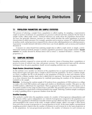
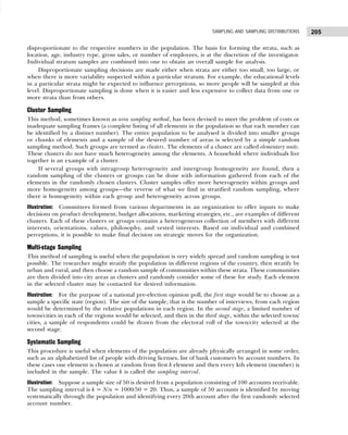
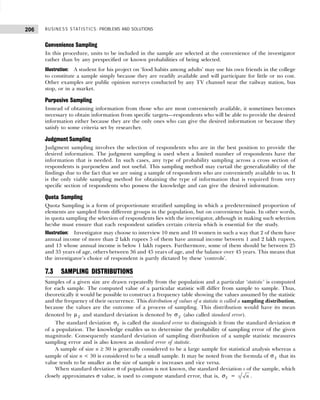
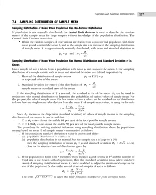
![BUSINESS STATISTICS: PROBLEMS AND SOLUTIONS
208
If σ is not known, the value of the normal variate z cannot be calculated for a specific sample. In such
a case, the standard deviation of population σ must be estimated using the sample standard deviation σ.
Thus, the standard error of the sampling distribution of mean x becomes
x
σ =
s
n
.
Since the value of x
σ varies according to each sample standard deviation, instead of using the
conversion formula
z =
/
x
n
− µ
σ
we use following formula, called ‘Student’s t-distribution’,
t =
/
x
s n
− µ
where s = Σ − −
2
( ) /( 1)
x x n .
Example 7.1: The mean length of life of a certain cutting tool is 41.5 hours with a standard deviation of
2.5 hours. What is the probability that a simple random sample of size 50 drawn from this population will
have a mean between 40.5 hours and 42 hours? [Delhi Univ., MBA, 2003]
Solution: We are given the following information, µ = 41.5 hours, σ = 2.5 hours, and n = 50.
It is required to find the probability that the mean length of life, x , of the cutting tool lies between 40.5
hours and 42 hours, that is, P(40.5 ≤ x ≤ 42).
Based upon the given information, the statistics of the sampling distribution are computed as
x
µ = µ = 41.5 and x
σ =
n
σ
=
2.5
50
=
2.5
7.0711
= 0.3536.
The population distribution is unknown, but sample size n = 50 is large enough to apply the central
limit theorem. Hence, the normal distribution can be used to find the required probability as shown by
the shaded area in Fig. 7.1.
P(40.5 ≤ x ≤ 42)= P 2
1
x x
x
x
z
−
−
≤ ≤
µ
µ
σ σ
= P
40.5 41.5 42 41.5
0.3536 0.3536
z
− −
≤ ≤
= P[– 2.8281 ≤ z ≤ 1.4140]
= P[z ≥ – 2.8281] + P[z ≤ 1.4140]
= 0.4977 + 0.4207 = 0.9184.
Thus, 0.9184 is the probability of the tool of
having a mean life between the required hours.
Example 7.2: A continuous manufacturing process
produces items whose weights are normally
distributed with a mean weight of 800 g and a
standard deviation of 300 g. A random sample of 16
items is to be drawn from the process.
(a) What is the probability that the arithmetic mean
of the sample exceeds 900 g? Interpret the
results.
(b) Find the values of the sample arithmetic mean
within which the middle 95 per cent of all
sample means will fall.
Figure 7.1 Normal Curve
Figure 7.2 Normal Curve](https://image.slidesharecdn.com/businessstatisticsproblemsandsolutions-230910073954-6d42a210/85/Business-Statistics_-Problems-and-Solutions-pdf-222-320.jpg)
![209
SAMPLING AND SAMPLING DISTRIBUTIONS
Solution: (a) We are given the following
information, µ = 800 g, σ = 300 g, and n = 16
Since population is normally distributed, the
distribution of sample mean is normal with mean
and standard deviation equal to
x
µ = µ = 800 and
x
σ =
n
σ
=
300
16
=
300
4
= 75.
The required probability, P( x > 900), is
represented by the shaded area in Fig. 7.2 of a
normal curve. Hence,
P( x > 900) = P
900 800
75
x
x
z
− −
> =
µ
σ
= P[z > 1.33]
= 0.5000 – 0.4082 = 0.0918.
Hence, 9.18 per cent of all possible samples of size n = 16 will have a sample mean value greater than
900 g.
(b) Since z = 1.96 for the middle 95 per cent area under the normal curve as shown in Fig. 7.3, using the
formula for z to solve for the values of x in terms of the known values are as follows:
x1 = x
µ – z x
σ = 800 – 1.96(75) = 653 g
and x2 = x
µ + z x
σ = 800 + 1.96(75) = 947 g.
Example 7.3: An oil refinary has backup monitors to keep track of the refinery flows continuously and
to prevent machine malfunctions from disrupting the process. One particular monitor has an average life
of 4300 hours and a standard deviation of 730 hours. In addition to the primary monitor, the refinery
has set up two standby units, which are duplicates of the primary one. In the case of malfunction of one
of the monitors, another will automatically take over in its place. The operating life of each monitor is
independent of the other.
(a) What is the probability that a given set of monitors will last at least 13,000 hours?
(b) At most 12,630 hours?
Solution: Given µ = 4300 hours, σ = 730 hours, n = 3. Based upon the given information, the statistics
of the sampling distribution are computed as
Mean, x
µ = µ = 4300 and x
σ =
x
σ
=
730
3
=
730
1.732
= 421.48.
(a) For a set of monitors to last 13,000 hours, they must each last 13,000/3 = 4333.33 hours on average.
The required probability is caluculated as follows:
P( x ≥ 4.333.33) = P
4333.33 4300
421.48
x
x
− −
≥
µ
σ
= P [ z ≥ 0.08] = 0.5 – 0.0319 = 0.4681.
(b) For the set to last at most 12,630 hours, the average life can not exceed 12,630/3 = 4210 hours.
The required probability is calculated as follows:
P( x ≤ 4210) = P
4210 4300
421.48
x
x
− −
≤
µ
σ
= P [ z ≤ – 0.213] = 0.5 – 0.0832 = 0.4168.
Figure 7.3 Normal Curve](https://image.slidesharecdn.com/businessstatisticsproblemsandsolutions-230910073954-6d42a210/85/Business-Statistics_-Problems-and-Solutions-pdf-223-320.jpg)
![BUSINESS STATISTICS: PROBLEMS AND SOLUTIONS
210
Example 7.4: Big Bazar, a chain of 130 shoping malls, has been bought out by another larger nationwide
supermarket chain. Before the deal is finalized, the larger chain wants to have some assurance that Big
Bazar will be a consistent money maker. The larger chain has decided to look at the financial records of
25 of the Big Bazar outlets. Big Bazar claims that each outlet’s profits have an apporximately normal
distribution with the same mean and a standard deviation of Rs. 40 million. If the Big Bazar management
is correct, then what is the probability that the sample mean for 25 outlets will fall within Rs. 30 million
of the actual mean?
Solution: Given N = 130, n = 25, σ = 40. Based upon the given information the statistics of the sampling
distribution are computed as
x
σ =
1
N n
N
n
−
−
σ
=
−
−
40 130 25
130 1
25
=
40 105
5 129
= 8 × 0.902 = 13.72.
The probability that the sample mean for 25 stores will fall within Rs. 30 million is given by
P(µ – 30 ≤ x ≤ µ + 30) = P
– 30 30
13.72 13.72
x
x
−
≤ ≤
µ
σ
= P(–2.18 ≤ z ≤ 2.18)
= 0.4854 + 0.4854 = 0.9708.
Example 7.5: Chief Executive officer (CEO) of a life insurance company wants to undertake a survey of
the huge number of insurance policies that the company has underwritten. The company makes an yearly
profit on each policy that is distributed with mean Rs. 8000 and standard deviation Rs. 300. It is desired
that the survey must be large enough to reduce the standard error to no more than 1.5 per cent of the
population mean. How large should the sample be?
Solution: Given µ = Rs. 8000 and σ = Rs. 300. The aim is to find sample size n be large enough so that
Standard error of estimate, x
σ =
n
σ
≤ 1.5 per cent of Rs. 8000
or
300
x
≤ 0.015 × 8000 = 120
300 ≤ 120 n or n ≥ 25 or n ≥ 625.
Thus, a sample size of at least 625 insurance policies is needed.
Example 7.6: Safal, a tea manufacturing company, is interested in determining the consumption rate of
tea per household in Delhi. The management believes that yearly consumption per household is normally
distributed with an unknown mean µ and standard deviation of 1.50 kg.
(a) If a sample of 25 household is taken to record their consumption of tea for one year, what is the
probability that the sample mean is within 500 g of the population mean?
(b) How large a sample must be in order to be 98 per cent certain that the sample mean is within 500 g
of the population mean?
Solution: Given µ = 500 gms, n = 25, and x
σ = σ/ n = 1.5/ 25 = 0.25 kg.
(a) Probability that the sample mean is within 500 g or 0.5 kg of the population mean is calculated as
follows:
P (µ – 0.5 ≤ x ≤ µ +0.5) = P
0.5 0.5
/ /
z
n n
−
≤ ≤
σ σ
= P
−
≤ ≤
0.5 0.5
0.25 0.25
z
= P [– 2 ≤ z ≤ 2] = 0.4772 + 0.4772 = 0.9544.
(b) For 98 per cent confidence, the sample size is calculated as follows:
P (µ – 0.5 ≤ x ≤ µ +0.5) = P
−
≤ ≤
0.5 0.5
1.5/ 1.5/
z
n n
.](https://image.slidesharecdn.com/businessstatisticsproblemsandsolutions-230910073954-6d42a210/85/Business-Statistics_-Problems-and-Solutions-pdf-224-320.jpg)
![211
SAMPLING AND SAMPLING DISTRIBUTIONS
Since z = 2.33 for 98 per cent area under normal curve,
2.33 =
0.5
1.5/ n
or 2.33 = 0.33 n
n = (2.33/0.33)2
= 49.84.
Hence, the management of the company should sample at least 50 households.
Example 7.7: A motorcycle manufacturing company claims that its particular brand of motorcycle gave
an average highway km per litre rating of 90. An independent agency tested it to verify the claim. Under
controlled conditions, the motorcycle was driven for a distance of 100 km on each of 25 different occasions.
The actual kms per litre achieved during the trip were recorded on each occasion. Over the 25 trials, the
average and standard deviation turned out to be 87 and 5 kms per litre, respectively. It is believed that the
distribution of the actual highway km per litre for this motorcycle is close to a normal distribution.
If the rating of 90 km per litre of the agency is correct, find the probability that the average kms per
litre over a random sample of 25 trials would be 87 or less.
Solution: Since the population standard deviation σ is unknown, t-Student’s test will be applicable to
calculate the desired probability P( x ≤ 87) as follows:
P( x ≤ 87) = P
/
x
t
s n
−
≤
µ
= P
−
≤
87 90
5/ 25
t = P[t ≤ –3]
with degrees of freedom (n – 1) = (25 – 1) = 24.
The desired probability of t ≤ –3.00 with df = 24 from t-distribution table is 0.0031. Hence, the
probability that the average km per litre is less than or equal to 87 is very small.
Sampling Distribution of Difference Between Two Sample Means
Let x1 and x2 be the mean of sampling distribution of mean of two populations, respectively. Then the
difference between their mean values µ1 and µ2 can be estimated by generalizing the formula of standard
normal variable as follows:
z = 1 2
1 2
1 2
( ) ( )
x x
x x
x x
−
− − −
µ µ
σ
=
1 2
1 2 1 2
( ) ( )
x x
x x
−
− − −
µ µ
σ
where 1 2
x x
−
µ = 1 2
x x
−
µ µ = µ1 – µ2 (mean of sampling distribution of difference of two means)
1 2
x x
−
σ =
1 2
2 2
x x
+
σ σ =
2
2
2
1
1 2
n n
+
σ
σ
(Standard error of sampling
distribution of two means)
n1, n2 = independent random samples drawn from first and second population,
respectively.
Since random samples are drawn independently from two populations with replacement, the sampling
distribution of the difference of two means 1 2
x x
− will be normal provided sample size is sufficiently large.
Example 7.8: Car stereos of manufacturer A have a mean lifetime of 1400 hours with a standard deviation
of 200 hours, while those of manufacturer B have a mean lifetime of 1200 hours with a standard deviation
of 100 hours. If a random sample of 125 stereos of each manufacturer are tested, what is the probability
that manufacturer A’s stereos will have a mean lifetime which is at least (a) 160 hours more than
manufacturer B’s stereos and (b) 250 hours more than the manufacturer B’s stereos?
[Delhi Univ., MBA, 1999]
Solution: We are given the following information
Manufacturer A: µ1 = 1400 hours, σ1 = 200 hours, n1 = 125
Manufacturer B: µ2 = 1200 hours, σ2 = 100 hours, n2 = 125
Thus, 1 2
x x
−
µ = 1 2
x x
−
µ µ = µ1 – µ2 = 1400 – 1200 = 200
1 2
x x
−
σ =
2
2
2
1
1 2
n n
+
σ
σ
=
2 2
(200) (100)
125 125
+ = 80 320
+ = 400 = 20.](https://image.slidesharecdn.com/businessstatisticsproblemsandsolutions-230910073954-6d42a210/85/Business-Statistics_-Problems-and-Solutions-pdf-225-320.jpg)
![BUSINESS STATISTICS: PROBLEMS AND SOLUTIONS
212
(a) Let 1
x – 2
x be the difference in mean lifetime
of stereo manufactured by the two manufacturers.
Then we are required to find the probability that this
difference is more than or equal to 160 hours, as
shown in Fig. 7.4. That is,
P[( 1
x – 2
x ) ≥ 160] = P
1 2
1 2 1 2
( ) ( )
x x
x x
z
−
− − µ − µ
≥
σ
= P
160 200
20
z
−
≥
= P[z ≥ – 2]
= 0.5000 + 0.4772
= 0.9772 (Area under normal curve).
Hence, the probability is very high that the mean
lifetime of the stereos of A is 160 hours more than
that of B.
(b) Proceeding in the same manner as in part (a) as
follows:
P[( 1
x – 2
x ) ≥ 250] = P
1 2
1 2 1 2
( ) ( )
x x
x x
z
−
− − −
≥
µ µ
σ
= P
250 200
20
z
−
≥
= P[z ≥ 2.5]
= 0.500 – 0.4938 = 0.0062.
Hence, the probability is very less that the mean lifetime of the stereos of A is 250 hours more than
that of B, as shown in Fig. 7.5.
Example 7.9: A particular brand of ball bearings weighs 0.5 kg with a standard deviation of 0.02 kg.
What is the probability that two lots of 1000 ball bearings each will differ in weight by more than 2 g.
Solution: We are given the following information
Lot 1: 1
x
µ = 1
µ = 0.50kg; σ1 = 0.02 kg; and n1 = 100
Lot 2: 2
x
µ = 2
µ = 0.50kg; σ2 = 0.02 kg; and n1 = 100
Thus, 1 2
x x
−
µ = 1 2
x x
−
µ µ = 1
µ – µ2 = 0
1 2
x x
−
σ =
2
2
2
1
1 2
n n
+
σ
σ
=
2 2
(0.02) (0.02)
1000 1000
+ = 0.000895.
A difference of 2 g in two lots is equivalent to a
difference of 2/100 = 0.002 kg in mean weights. It is
possible if 1 2
x x
− ≤ 0.002 or 1 2
x x
− ≥ – 0.002. Then the
required probability that each ball bearing will differ by
more than 2 g is calculated as follows and is shown in
Fig. 7.6.
P − ≤ − ≤
1 2
0.002 0.002
x x
= P
( ) ( ) ( ) ( )
1 2 1 2
1 2 1 2 1 2 1 2
x x x x
x x x x
z
− −
− − − − − −
≤ ≤
µ µ µ µ
σ σ
= P
−
≤ ≤
0.002 0.002
0.000895 0.000895
z = P [– 2.33 ≤ z ≤ 2.33]
= 2 [0.5000 – 0.4871] = 0.0258.
Figure 7.4 Normal Curve
Figure 7.5 Normal Curve
Figure 7.6 Normal Curve](https://image.slidesharecdn.com/businessstatisticsproblemsandsolutions-230910073954-6d42a210/85/Business-Statistics_-Problems-and-Solutions-pdf-226-320.jpg)
![213
SAMPLING AND SAMPLING DISTRIBUTIONS
7.1 A diameter of a component produced on a semi-
automatic machine is known to be distributed normally
with a mean of 10 mm and a standard deviation of 0.1
mm. If a random sample of size 5 is picked up, what is
the probability that the sample mean will be between
9.95 mm and 10.05 mm? [Delhi Univ., MBA, 1997]
7.2 The time between two arrivals at a queuing system is
normally distributed with a mean of 2 minutes and
standard deviation 0.25 minute. If a random sample
of 36 is drawn, what is the probability that the sample
mean will be greater than 2.1 minutes?
7.3 The strength of the wire produced by company A has
a mean of 4500 kg and a standard deviation of 200
kg. Company B has a mean of 4000 kg and a standard
deviation of 300 kg. If 50 wires of company A and
100 wires of company B are selected at random and
tested for strength, what is the probability that the
sample mean strength of A will be atleast 600 kg more
than that of B? [Delhi Univ., MBA, 2000]
7.4 For a certain aptitude test, it is known from past
experience that the average score is 1000 and the
standard deviation is 125. If the test is administered to
100 randomly selected individuals, what is the
probability that the value of the average score for this
sample will lie in the interval 970 and 1030? Assume
that the population distribution is normal.
7.5 A manufacturing process produces ball bearings with
mean 5 cm and standard deviation 0.005 cm. A
random sample of 9 bearings is selected to measure
their average diameter and find it to be 5.004 cm.
What is the probability that the average diameter of 9
randomly selected bearings would be at least 5.004 cm?
7.6 A population of items has an unknown distribution
but a known mean and standard deviation of 50 and
100, respectively. Based upon a randomly drawn
sample of 81 items drawn from the population, what
is the probability that the sample arithmetic mean does
not exceed 40?
7.7 A marketing research team has determined the
standard error of sampling distribution of mean for a
proposed market research sample size of 100
consumers. However, this standard error is twice the
level that the management of the organization
considers acceptable. What can be done to achieve an
acceptable standard error for mean?
7.8 Assume that the height of 300 soldiers in an army
batallion are normally distributed with mean 68 inches
and standard deviation 3 inches. If 80 samples
consisting of 25 soldiers each are taken, what would
be the expected mean and standard deviation of the
resulting sampling distribution of means if the
sampling is done (a) with replacement and (b) without
replacement?
7.9 How well have equity mutual funds performed in the
past compared with BSE Stock Index? A random
sample of 36 funds averages a 16.9 per cent annual
investment return for 2001–02 with a standard
deviation of 3.6 per cent annual return. The BSE Stock
Index grew at an annual average rate of 16.3 per cent
over the same period. Do these data show that, on the
average, the mutual funds out-performed the BSE
Stock Index during this period?
7.10 The average annual starting salary for an MBA is
Rs. 3,42,000. Assume that for the population of MBA
(Marketing majors), the average annual starting salary
is µ = 3,40,000 and the standard deviation is σ =
20,000. What is the probability that a simple random
sample of MBA (Marketing majors) will have a sample
mean within ± Rs. 2,500 of the population mean for
each sample sizes: 50,100, and 200? What is your
conclusion? [Delhi Univ., MBA, 2003]
7.1 Given x
µ = µ = 10, σ = 0.1, and n = 10. Thus,
x
σ = / n
σ = 0.1/ 5 = 0.047
P[9.95 ≤ x ≤ 10.05]
= P
1 2
2
1
x x
x
x
z
−
−
≤ ≤
µ
µ
σ σ
= P
− −
≤ ≤
9.95 10 10.05 10
0.047 0.047
z
= P[–1.12 ≤ z ≤ 1.12]
= P[z ≥ – 1.12] + P[z ≤ 1.12]
= 0.3686 + 0.3686 = 0.7372
S e l f-P r a c t i c e P r o b l e m s 7A
Hints and Answers](https://image.slidesharecdn.com/businessstatisticsproblemsandsolutions-230910073954-6d42a210/85/Business-Statistics_-Problems-and-Solutions-pdf-227-320.jpg)
![BUSINESS STATISTICS: PROBLEMS AND SOLUTIONS
214
7.2 Given x
µ = µ = 2, σ = 0.25, and n = 36. Thus,
x
σ =
3,37,000 3,40,000
/
20,000 / 50
n
−
σ
= 0.25/ 36 = 0.042
P[ x ≥ 2.1] = P
x
x
z
−
≥
µ
σ
= P
−
≥
2.1 2
0.042
z
= P[z ≥ 2.38] = 0.5000 – 0.4913
= 0.0087
7.3 Given µ1 = 4500, σ1 = 200, and n1 = 50 ; µ2 = 4000,
σ2 = 300, and n2 = 100. Then
1 2
x x
−
µ = µ1 – µ2 = 4500 – 4000 = 500
1 2
x x
−
σ =
2
2
2
1
1 2
n n
+
σ
σ
= +
40,000 90,000
50 100
= 41.23
P[( −
1 2
x x ) ≥ 600] = P
1 2
1 2 1 2
( ) ( )
x x
x x
z
−
− − −
≥
µ µ
σ
= P
−
≥
600 500
41.23
z = P(z ≥ 2.43)
= 0.5000 – 0.4925 = 0.0075
7.4 Given x
µ = µ = 1000, σ = 125, and n = 100. Thus,
x
σ = / n
σ = 125/ 100 = 12.5
P(970 ≤ x ≤ 1030) = P 2
1
x x
x
x
z
−
−
≤ ≤
µ
µ
σ σ
= P
− −
≤ ≤
970 1000 1030 1000
12.5 12.5
z
= P(–2.4 ≤ z ≤ 2.4) = P(z ≤ 2.4) + P(z ≥ – 2.4)
= 0.4918 + 0.4918 = 0.9836
7.5 Given x
µ = µ = 5, σ = 0.005, and n = 9. Thus,
x
σ = / n
σ = 0.005/ 9 = 0.0017
P( x ≥ 5.004) = P
− µ
≥
σ
x
x
z
=
−
≥
5.004 5.000
0.0017
P z
= P(z ≥ 2.4) = 1 – P(z ≤ 2.4)
= 1 – 0.9918 = 0.0082
7.6 Given x
µ = µ = 50, σ = 100, and n = 81. Thus,
x
σ = / n
σ = 100/ 81 = 11.1
P( x ≤ 40) = P
x
x
z
−
≥
µ
σ
=
−
≤
40 50
11.1
P z
= P(z ≤ – 0.90) = 0.5000 – 0.3159
= 0.1841
7.7 Since standard error is inversely proportional to the
square root of the sample size, to reduce the standard
error determined by the market research team, the
sample size should be increased to n = 400 (four times
of n = 100).
7.8 The number of possible samples of size 25 each from
a group of 3000 soldiers with and without replacement
are (3000)25
and 300
C25, respectively. These numbers
are much larger than 80—actually drawn samples.
Thus we will get only an experimental sampling
distribution of means rather than true sampling
distribution. Hence mean and standard deviation
would be close to those of the theoretical distribution.
That is,
(a) x
µ = µ = 68 and
x
σ = / n
σ = 3/ 25 = 0.60
(b) x
µ = µ = 68 and x
σ =
1
N n
N
n
−
−
σ
=
−
−
3000 25
3
3000 1
25
= 1.19
7.9 Given x
µ = µ = 16.9, σ = 3.6, and n = 36. Thus,
x
σ = / n
σ = 3. 6 / 36 = 0.60
P( x ≥ 16.3) = P
x
x
z
−
≥
µ
σ
= P
−
≥
16.3 16.9
0.60
z
= P[z ≥ – 1] = 0.5000 + 0.1587 = 0.6587
7.10 Given µ = 3,40,000, σ = 20,000, n1 = 50, n2 = 100,
and n3 = 200
For n1 = 50,
z1 =
x
x − µ
σ
=
−
3,42,000 3,40,000
20,000 / 50
= 0.88
z2 =
−
3,37,000 3,40,000
20,000 / 50
= – 0.88
P(– 0.88 ≤ z ≤ 0.88) = 0.3106 × 2 = 0.6212
Similar calculations for n2 = 100 and n2 = 200
give
P(–1.25 ≤ z ≤ 1.25) = 0.3944 × 2 = 0.7888
P(–1.76 ≤ z ≤ 1.76) = 0.4616 × 2 = 0.9282.](https://image.slidesharecdn.com/businessstatisticsproblemsandsolutions-230910073954-6d42a210/85/Business-Statistics_-Problems-and-Solutions-pdf-228-320.jpg)
![215
SAMPLING AND SAMPLING DISTRIBUTIONS
7.5 SAMPLING DISTRIBUTION OF SAMPLE PROPORTION
If a random sample of n elements is selected from the binomial population and x of these possess the
specified characteristic, then the sample proportion p is the best statistic to use for statistical inferences
about the population proportion parameter p. The sample proportion can be defined as
p =
Elements of sample having characteristic,
Sample size,
x
n
.
With the same logic of sampling distribution of mean, the sampling distribution of sample proportions
with mean p
µ and standard deviation (also called standard error) p
σ is given by
p
µ = p and p
σ =
pq
n
=
(1 )
p p
n
−
.
If the sample size n is large (n ≥ 30), the sampling distribution of p can be approximated by a normal
distribution. The approximation will be adequate if np ≥ 5 and n(1 – p) ≥ 5.
The mean and standard deviation (error) of the sampling distribution of proportion are valid for a
finite population in which sampling is with replacement. However, for finite population in which sampling
is done without replacement, we have
p
µ = p and p
σ =
−
−1
pq N n
n N
.
Under the same guidelines as mentioned in previous sections, for a large sample size n (≥ 30), the
sampling distribution of proportion is closely approximated by a normal distribution with mean and
standard deviation as stated above. Hence, to standardize sample proportion p, the standard normal variable
z =
p
p
p − µ
σ
=
(1 )/
p p
p p n
−
−
is approximately the standard normal distribution.
Sampling Distribution of the Difference of Two Proportions
Suppose two populations of size N1 and N2 are given. For each sample of size n1 from first population,
compute sample proportion 1
p and standard deviation 1
p
σ . Similarly, for each sample of size n2 from
second population, compute sample proportion 2
p and standard deviation 2
p
σ .
For all combinations of these samples from these populations, we can obtain a sampling distribution
of the difference 1
p – 2
p of sample proportions. Such a distribution is called sampling distribution of
difference of two proportions. The mean and standard deviation of this distribution are given by
1 2
p p
−
µ = 1 2
p p
−
µ µ = p1 – p2
and 1 2
p p
−
σ =
1 2
2 2
p p
+
σ σ =
2 2
1 1
1 2
(1 )
(1 ) p p
p p
n n
−
−
+ .
If sample size n1 and n2 are large, that is, n1 ≥ 30 and n2 ≥ 30, then the sampling distribution of
difference of proportions is closely approximated by a normal distribution.
Example 7.10: A manufacturer of watches has determined from experience that 3 per cent of the watches
he produces are defective. If a random sample of 300 watches is examined, what is the probability that the
proportion defective is between 0.02 and 0.035? [Delhi Univ., MBA, 1990]
Solution: We are given the following information
p
µ = p = 0.03, 1
p = 0.02, 2
p = 0.035, and n = 300.](https://image.slidesharecdn.com/businessstatisticsproblemsandsolutions-230910073954-6d42a210/85/Business-Statistics_-Problems-and-Solutions-pdf-229-320.jpg)
![BUSINESS STATISTICS: PROBLEMS AND SOLUTIONS
216
Thus, standard error of proportion is given by
p
σ =
(1 )
p p
n
−
=
0.03 0.97
300
×
= 0.000097 = 0.0098.
For calculating the desired probability, we apply the following formula
Figure 7.7 Normal Curve
P[0.02 ≤ p ≤ 0.035] = P
−
−
≤ ≤
σ σ
2
1
p p
p p
p p
z = P
− −
≤ ≤
0.02 0.03 0.035 0.03
0.0098 0.0098
z
= P[–1.02 ≤ z ≤ 0.51] = P(z ≥ – 1.02) + P(z ≤ 0.51) = 0.3461 + 0.1950 = 0.5411.
Hence the probability that the proportion of defectives will lie between 0.02 and 0.035 is 0.5411
(Fig. 7.7).
Example 7.11: Few years back, a policy was introduced to give loan to unemployed engineers to start
their own business. Out of 1,00,000 unemployed engineers, 60,000 accepted the policy and got the loan.
A sample of 100 unemployed engineers is taken at the time of allotment of loan. What is the probability
that sample proportion would have exceeded 50 per cent acceptance?
Solution: We are given the following information
p
µ = p = 0.60, N = 1,00,000, and n = 100.
Thus, the standard error of proportion in a finite population of size 1,00,000 is given by
p
σ =
( )
1 N
N 1
p p n
n
− −
−
=
× −
−
0.60 0.40 1,00,000 100
100 1,00,000 1
= 0.0024 0.9990 = 0.0489 × 0.9995 = 0.0488.
The probability that sample proportion would have exceeded 50 per cent acceptance is given by
P(x ≥ 0.50) = P
−
≥
σ
p
p p
z = P
−
≥
0.50 0.60
0.0489
z = P[z ≥ – 2.04] = 0.5000 + 0.4793 = 0.9793.
Example 7.12: Ten per cent of machines produced by company A are defective and five per cent of those
produced by company B are defective. A random sample of 250 machines is taken from company A and
a random sample of 300 machines from company B. What is the probability that the difference in sample
proportion is less than or equal to 0.02? [South Gujrat Univ., MBA; Delhi Univ., MBA, 1999]
Solution: We are given the following information
1 2
p p
−
µ = 1 2
p p
−
µ µ = p1 – p2 = 0.10 – 0.05 = 0.05; n1 = 250; and n2 = 300
Thus, standard error of the difference in a sample proportion is given by
1 2
p p
−
µ =
2 2
1 1
1 2
(1 )
(1 ) p p
p p
n n
−
−
+ =
0.10 0.90 0.05 0.95
250 300
× ×
+](https://image.slidesharecdn.com/businessstatisticsproblemsandsolutions-230910073954-6d42a210/85/Business-Statistics_-Problems-and-Solutions-pdf-230-320.jpg)
![217
SAMPLING AND SAMPLING DISTRIBUTIONS
=
0.90 0.0475
250 300
+ = 0.00052 = 0.0228.
The desired probability of difference in sample proportions is given by
Figure 7.8 Normal Curve
P[( 1
p – 2
p ) ≤ 0.02] = P
1 2
1 2 1 2
( ) ( )
p p
p p p p
z
−
− − −
≤
σ
= P
0.02 0.05
0.0228
z
−
≤
= P[z ≤ – 1.32]
= 0.5000 – 0.4066 = 0.0934.
Hence, the desired probability for the difference in sample proportions is 0.0934 (Fig. 7.8).
7.6 MISCELLANEOUS SOLVED EXAMPLES
Example 7.13: The nine items of a sample had the following values: 45, 47, 50, 52, 48, 47, 49, 53, 51,
does the mean of the nine items differ significantly from the assumed population mean 47.5?
Given that when degree of freedom (df)8; A = 0.945 for t = 1.8, A = 0.953 for t = 1.9,
where A is the area to the left of the ordinate at t.
Solution: Since sample size is small, applying t test as t =
/
x
s n
− µ
...(i)
The values of x and σ are calculated as given below:
x d = x – A d2
45 –3 9
47 –1 1
50 2 4
52 4 16
48 ← A 0 0
47 –1 1
49 1 1
53 5 25
51 3 9
Total 10 66
If A = 48 is the assumed mean, then
Mean, x =
10
48 48 1.111 49.111
9
d
A
n
∑
+ = + = + =
Variance, σ2
=
2 2
2 ( ) (10)
1 1
66
1 8 9
d
d
n n
∑
∑ − = −
− ](https://image.slidesharecdn.com/businessstatisticsproblemsandsolutions-230910073954-6d42a210/85/Business-Statistics_-Problems-and-Solutions-pdf-231-320.jpg)
![BUSINESS STATISTICS: PROBLEMS AND SOLUTIONS
218
=
1
8
[66 – 11.111] =
1
8
[54.889] = 6.861
SD, σ = (6.861) = 2.619.
Thus, t =
3(1.611)
49.111 47.5
= =
2.619
/ 2.619/ 9
x
s n
− −
µ
= 1.845 = 1.85.
The difference in the value of A for 0.1 = 0.953 – 0.945 at 8 df = 0.008
and difference in the value of A for 1.85 – 1.80 = 0.05
=
0.008
0.05
0.1
× = 0.004.
Hence, when t = 1.85, A = 0.945+0.004 = 0.949
Probable error PE = 2 (1 – As) = 2 (1 – 0.949) = 2(0.051) = 0.102 > 0.05.
Therefore, the value of t is not significant at 5% level of significance and so the test provides no
evidence against the population mean being 47.5.
Example 7.14: Ten individuals are chosen at random from a population and their heights are found to
be in inches : 63, 63, 66, 67, 68, 69, 71, 70, 71, 70.
In the light of these data, discuss the suggestion that the mean height in the population in 66 inches
having given that for t = 1.8, A = 0.947, and for t = 1.9, A = 0.955, where A is the area to the left of the
ordinate at t.
Solution: Since sample size is small, applying t-test as t =
/
x
s n
− µ
The values of x and s are calculated as given below:
x d = x – A = x – 67 d2
63 –4 16
63 –4 16
66 –1 1
67 ← A 0 0
68 1 1
69 2 4
71 4 16
70 3 9
71 4 16
70 3 9
Total 8 88
If A = 67 is the assumed mean, then
x = 8
67 67.8 inches
10
d
A
n
∑
+ = + =
Variance, s2
=
2 2
2 ( ) (8)
1 1
88
1 10 1 10
d
d
n n
∑
∑ − = −
− −
= [ ] [ ]
1 1
88 6.4 81.6 9.066
9 9
− = =
SD, s = (9.066) 3.011
= .
Thus, t = 67.8 66
=
/ 3.011 10
x
s n
− −
µ
= 5.692
=1.89
3.011
.](https://image.slidesharecdn.com/businessstatisticsproblemsandsolutions-230910073954-6d42a210/85/Business-Statistics_-Problems-and-Solutions-pdf-232-320.jpg)
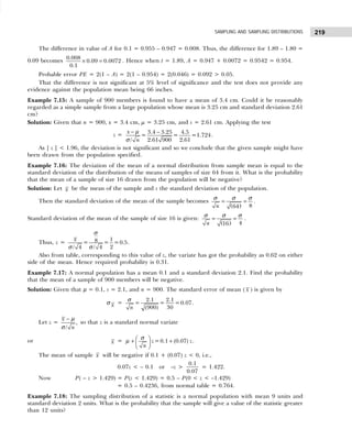
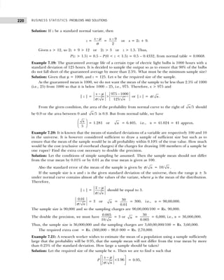
![221
SAMPLING AND SAMPLING DISTRIBUTIONS
where x is the mean of the sample of size n; µ and σ are the mean and standard deviations of the
population from which the sample is drawn.
Also it is given that | x – µ | ≤ 1
4
σ or
1.96
n
σ
≤
4
σ
or = 4(1.96)
n , i.e. n = 61.465.
Hence, n = 62 is the required minimum size of the sample.
Example 7.22: Suppose that the standard deviation of stature in men is 2.48 inches. One hundred male
students in a large university are measured and their average height is found to be 68.52 inches. Determine
the 98% confidence limits for the mean height of the mean of the university.
Solution: Given that s = 2.48, n = 100, and x = 68.52. Therefore standard error of the mean height of
100 male students becomes
2.48
= =0.248 inches.
(100)
n
σ
At 98% confidence limits for the mean height of the mean of the university implies that 49% of the
total area under the normal curve lies on each side of the mean. Thus, 0.5 + 0.49 = 0.99, area under the
standard normal curve lies to the left of the critical value of the variate z or the area under the standard
normal curve from the mean zero to the ordinate under consideration is 0.49. And from the table we find
that this critical value of z is 2.32.
For the required limits, we have
68.52
0.248
n
−
< 2.32
68.52 – 2.32 (0.248) < µ < 68.52 + 2.32 (0.248)
68.52 – 0.575 < µ < 68.52 + 0.575
67.945 > µ < 69.095.
Hence, the required 98% confidence limits for the mean height of the men of university are 67.945
inches and 69.095 inches.
Example 7.23: The standard deviation of a population is 2.70 inches. Find the probability that in samples
of size 66, the sample mean will differ from population mean by 0.75 inch or more. Given that the value
of the normal probability integral from 0 to 2.25 is 0.4877.
Solution: According to the questions we need to have
0.75]
P x µ
− ≥ = 1 [ 0.75]
P x
− − ≤
µ = 1 / 0.75
P n z
− <
σ
=
0.75
1
n
P z
− <
σ
=
− <
0.75 (66)
1 2
2.70
P z
=
− <
0.75 (8.12)
1 2
2.70
P z =
6.90
1 2
2.70
P z
− <
= [ ]
1 2 2.25
P z
− <
= 1 – 2(0.4877) = 1 – 0.9754 = 0.0246.
Example 7.24: To know the mean weight of all 10 year old boys in the state of Rajasthan a sample of 225
is taken. The mean weight of this sample is found to be 67 pounds with a standard deviation of 12
pounds. Can any inference be drawn from it about the mean weight of the universe?
Solution: Given standard deviation of the sample is 12 pounds, which can be taken to be the standard
deviation of the universe as it is not known. Thus,
Standard error of the mean =
12 12
15
(225)
n
= =
σ = 0.8 pound.](https://image.slidesharecdn.com/businessstatisticsproblemsandsolutions-230910073954-6d42a210/85/Business-Statistics_-Problems-and-Solutions-pdf-235-320.jpg)
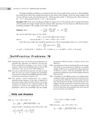
![223
SAMPLING AND SAMPLING DISTRIBUTIONS
P( p ≤ 12)= P
p
p np
z
−
≤
σ
= P
−
≤
12 10
2.24
z
= P(z ≤ 0.89) = 0.8133
7.13 Given p
µ = p = 0.30, n = 500;
p
σ =
−
(1 )
p p
n
=
×
0.30 0.70
500
= 0.0205.
P( p ≤ 0.25) = P
p
p p
z
−
≤
σ
=
−
≤
0.25 0.30
0.0205
z
=P[z ≤ – 2.43] = 0.5000 – 0.4927 = 0.0083
7.14 Given p
µ = p = 0.04, n = 400;
p
σ =
−
(1 )
p p
n
=
×
0.04 0.96
400
= 0.009
P[0.02 ≤ p ≤ 0.05] = P
−
−
≤ ≤
σ σ
2
1
p p
p p
p p
z
= P
− −
≤ ≤
0.02 0.04 0.05 0.04
0.009 0.009
z
= P[– 2.22 ≤ z ≤ 2.22]
=P[z ≥ – 2.22] + P[z ≤ 2.22]
= 0.4861 + 0.4861 = 0.9722
7.15 Given p
µ = p = 0.20, n = 140;
p
σ =
−
(1 )
p p
n
=
×
0.20 0.80
140
= 0.033
P[ p ≥ 0.28] = P
p
p p
z
−
≥
σ
= P
−
≥
0.28 0.20
0.033
z = P[z ≥ 2.42]
=0.5000 – 0.4918 = 0.0082](https://image.slidesharecdn.com/businessstatisticsproblemsandsolutions-230910073954-6d42a210/85/Business-Statistics_-Problems-and-Solutions-pdf-237-320.jpg)
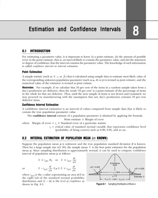
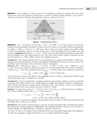
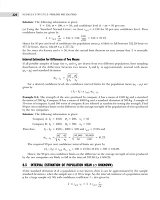
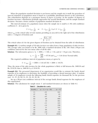
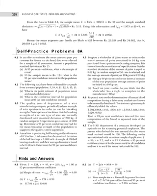
![229
ESTIMATION AND CONFIDENCE INTERVALS
x ± tα/2
s
n
= 10 ± 2.365
3.46
8
= 10 ± 2.90; 7.10 ≤ µ ≤ 12.90
8.3 Given x = 6200, σ = 200, n = 64, and zα /2 = 1.96 at
95 per cent confidence coefficient
x ± zα/2
n
σ
= 6200 ± 1.96
200
64
= 6200 ± 49; 6151 ≤ µ ≤ 6249
8.4 Given x = 0.498, σ = 0.005, n = 100, zα/2 = 2.58 at
99 per cent confidence coefficient
x ± zα/2
n
σ
= 0.498 ± 2.58
0.005
100
= 0.498 ± 0.0129; 0.4967 ≤ µ ≤ 0.4993
8.5 Given x = 0.995, σ = 0.02, n = 50, and zα/2 = 2.58 at
99 per cent confidence coefficient
(a) x ± zα/2
n
σ
= 0.995 ± 2.58
0.02
100
= 0.995 ± 0.0072; 0.9878 ≤ µ ≤ 1.0022
(b) Since the value 1.0 is included in the interval, there
is no need to believe that the average is below 1.0.
8.6 x =
∑ x
n
=
10.107
10
= 1.010,
s =
Σ −
−
2
( )
( 1)
x x
n
= 0.025; n = 10
tα/2 = 3.250 at df = 9 and 99 per cent confidence
coefficient
x ± tα /2
s
n
= 1.010 ± 3.250
0.025
100
= 1.010 ± 0.025; 0.985 ≤ µ ≤ 1.035
8.7 Given x = 96, s = 5.2, n = 13, zα/2 = 1.96 at
95 per cent confidence coefficient
x ± zα /2
s
n
= 96 ± 1.96
5.2
13
= 96 ± 2.83; 93.17 ≤ µ ≤ 98.83.
8.4 INTERVAL ESTIMATION FOR POPULATION PROPORTION
When np ≥ 5 and nq = n(1 – p) ≥ 5, the central limit theorem for sample proportions gives us the formula
z =
−
/
p p
pq n
When the sample size is large, the sample proportion
p = x/n is the best point estimator for the population
proportion p (Fig. 8.3). Since the sampling
distribution of sample proportion p is approximately
normal with mean p
µ and standard error /
pq n ,
the confidence interval for a population proportion
at 1 – α confidence coefficient is given by
p ± zα/2 p
µ = p ± zα/2 /
pq n
or p – zα/2 p
σ ≤ p ≤ p + zα/2 p
σ .
Since p and q are unknown, they are estimated
using the point estimator: p and q . Thus for a sample proportion, the standard error denoted by SE ( p )
or p
σ is given by
p
σ = /
p q n = −
(1 ) /
p p n .
Example 8.7: Suppose in a town we want to estimate the proportion of families that have two or more
children. A random sample of 144 families shows that 48 families have two or more children. Set up a
95 per cent confidence interval estimate of the population proportion of families having two or more
children. [HP Univ., MBA, 1999]
Solution: The sample proportion is p = x/n = 48/144 = 1/3. Using the information,
n = 144, p = 1/3, and zα/2 = 1.96 at 95 per cent confidence coefficient, we have
p ± zα/2
(1 )
p p
n
−
=
1
3
± 1.96
( )( )
1/ 3 2/ 3
144
= 0.333 ± 0.077.
Hence the population proportion of families who have two or more children is likely to be between
25.6 to 41 per cent, that is, 0.256 ≤ p ≤ 0.410.
Figure8.3 SamplingDistributionofProportion p](https://image.slidesharecdn.com/businessstatisticsproblemsandsolutions-230910073954-6d42a210/85/Business-Statistics_-Problems-and-Solutions-pdf-243-320.jpg)
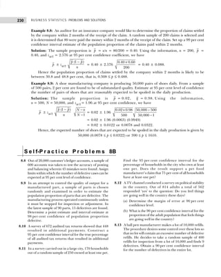
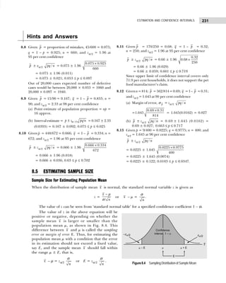
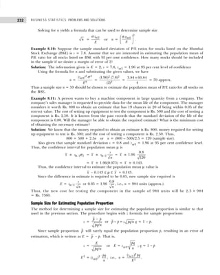
![233
ESTIMATION AND CONFIDENCE INTERVALS
Example 8.12: A car manufacturing company received a shipment of petrol filters. These filters are to be
sampled to estimate the proportion that is unusable. From past experience, the proportion of unusable
filter is estimated to be 10 per cent. How large a random sample should be taken to estimate the true
proportion of unusable filters to within 0.07 with 99 per cent confidence.
Solution: The information given is E=0.07, p=0.10, and zα/2 = 2.576 at 99 per cent confidence level.
Using the formula for n and substituting the given values, we have
n =
2
/2
2
( )
z pq
E
α
=
2
2
(2.576) (0.10 0.90)
(0.07)
×
= 121.88.
Therefore, a slightly larger sample size of n=122 filters should be taken.
Sample Size Determination for Finite Population
This uses finite population correction factor when samples are drawn without replacement from a finite
population of size N reduces the standard error by a value equal to − −
( )/( 1)
N n N . For example, for
deciding sample size n for estimating the population mean µ, the desired margin of error is given by
E = /2
1
z N n
N
n
−
−
α σ
.
Similarly, when estimating the proportion, the desired margin of error is given by
p
σ or E = zα/2
−
−1
pq N n
n N
.
Let n0 be the size for estimating population mean without using correction factor. Then
n0 =
2 2
/2
2
( )
z
E
α σ
.
The revised sample size, taking into consideration the size of the population, is given by
n =
+ −
0
0 ( 1)
n N
n N
.
Example 8.13: For a population of 1000, what should be the sampling size necessary to estimate the
population mean at 95 per cent confidence with a sampling error of 5 and the standard deviation equal to 20?
Solution: We have E = 5, σ = 20, zα/2 = 1.96 at 95 per cent confidence level, and N = 1000. Thus,
n =
2 2
/2
2
( )
z
E
α σ
=
2 2
2
(1.96) (20)
(5)
= 61.456.
Since the population size is finite, the revised sample size obtained by using the correction factor
n =
+ −
0
0 ( 1)
n N
n N
=
(61.456) (1000)
61.456 (1000 1)
+ −
=
61456
1060.456
= 57.952.
Thus, a slightly larger sample size of n = 58 should be taken.
S e l f-P r a c t i c e P r o b l e m s 8C
8.14 Given a population with a standard deviation of 8.6.
What sample size is needed to estimate the mean of
population within ±0.5 with 99 per cent confidence?
[Delhi Univ., M.Com., 1999]
8.15 A cigarette manufacturer wishes to use random
sampling to estimate the average nicotine content. The
sampling error should not be more than one milligram
above or below the true mean with a 99 per cent
confidence coefficient. The population standard
deviation is 4 milligrams. What sample size should the
company use in order to satisfy these requirements?
8.16 A firm wishes to estimate with a maximum allowable
error of 0.05 and a 95 per cent level of confidence, the
proportion of consumers who prefer its product. How
large a sample will be required in order to make such
an estimate if the preliminary sales reports indicate
that 25 per cent of all consumers prefer the firm’s
product?](https://image.slidesharecdn.com/businessstatisticsproblemsandsolutions-230910073954-6d42a210/85/Business-Statistics_-Problems-and-Solutions-pdf-247-320.jpg)
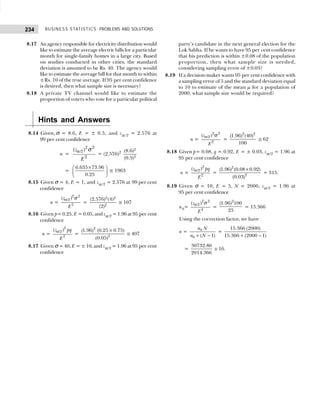
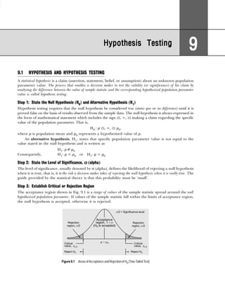
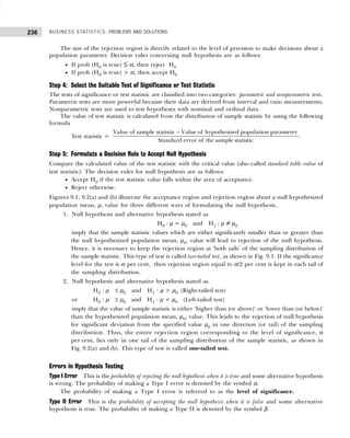
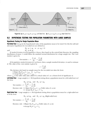
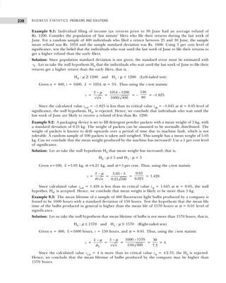
![239
HYPOTHESIS TESTING
Example 9.4: A continuous manufacturing process of steel rods is said to be in ‘state of control’ and
produces acceptable rods if the mean diameter of all rods procuced is 2 inches. Although the process
standard deviation exhibits stability over time with standard deviation, σ = 0.01 inch. The process mean
may vary due to operator error or problems of process adjustment. Periodically, random samples of 100
rods are selected to determine whether the process is producing acceptable rods. If the result of a test
indicates that the process is out of control, it is stopped and the source of trouble is sought. Otherwise, it
is allowed to continue operating. A random sample of 100 rods is selected resulting in a mean of 2.1
inches. Test the hypothesis to determine whether the process be continued.
Solution: Since rods that are either too narrow or too wide are unacceptable, the low values and high
values of the sample mean lead to the rejection of the null hypothesis. Consider the null hypothesis H0,
that the process may be allowed to continue when diameter is 2 inches. Consequencly, rejection region is
on both tails of the sampling distribution. The null and alternative hypotheses are stated as follows:
H0 : µ = 2 inches, (continue process)
H1 : µ ≠ 2 inches, (stop the process)
Given n = 100, x = 2.1, σ = 0.01, α = 0.01. Using the z-test statistic
z =
x
x − µ
σ
=
/
x
n
− µ
σ
=
2.1 2
0.01/ 100
−
=
0.1
0.001
= 100.
Since zcal=100 value is more than its critical value zα/2 = 2.58 at α = 0.01, the null hypothesis, H0, is
rejected. Thus stop the process in order to determine the source of trouble.
Example 9.5: An ambulance service claims that it takes, on the average, 8.9 minutes to reach its destination
in emergency calls. To check on this claim, the agency which licenses ambulance services has then timed
on 50 emergency calls, getting a mean of 9.3 minutes with a standard deviation of 1.8 minutes. Does this
constitute evidence that the figure claimed is too low at the 1 per cent significance level?
Solution: Let us consider the null hypothesis H0 that ‘the claim is same as observed’ and alternative
hypothesis is ‘claim is different than observed’. These two hypotheses are written as
H0 : µ = 8.9 and H1 : µ ≠ 8.9
Given n = 50, x = 9.3, and s = 1.8. Using the z-test statistic, we get
z =
x
x
s
− µ
=
/
x
s n
− µ
=
9.3 8.9
1.8 / 50
−
=
0.4
0.254
= 1.574.
Since zcal = 1.574 in less than its critical value zα/2 = ±2.58, at α = 0.01, the null hypothesis is
accepted. Thus, there is no difference between the average time observed and claimed.
Example 9.6: An auto company decided to introduce a new six cylinder car whose mean petrol
consumption is claimed to be lower than that of the existing auto engine. It was found that the mean
petrol consumption for 50 cars was 10 km per litre with a standard deviation of 3.5 km per litre. Test for
the company, at 5 per cent level of significance, the claim that in the new car petrol consumption is 9.5
km per litre on the average. [HP Univ., MBA, 1989]
Solution: Let us assume the null hypothesis H0 that there is no significant difference between the company’s
claim and the sample average value, that is,
H0 : µ = 9.5 km/litre and H1 : µ ≠ 9.5 km/litre
Given x = 10, n = 50, s = 3.5, and zα/2 = 1.96 at α = 0.05 level of significance. Thus, using the
z-test statistic
z =
x
x − µ
σ
=
/
x
s n
− µ
=
10 9.5
3.5/ 50
−
= 1.010.
Since zcal = 1.010 is less than its critical value zα/2 = 1.96 at α = 0.05 level of significance, the null
hypothesis is accepted. Hence we can conclude that the new car’s petrol consumption is 9.5 km/litre.](https://image.slidesharecdn.com/businessstatisticsproblemsandsolutions-230910073954-6d42a210/85/Business-Statistics_-Problems-and-Solutions-pdf-253-320.jpg)
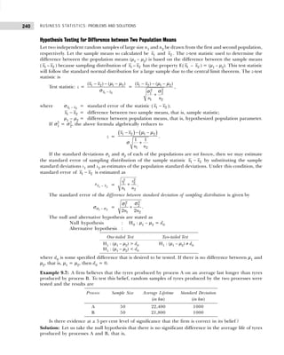
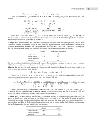
![BUSINESS STATISTICS: PROBLEMS AND SOLUTIONS
242
Do the data support the conclusion that given populations of female and male students with similar
high ability in mathematics, the female students will have a significantly high verbal ability? Test at
α = 0.05 significance level. What is your conclusion? [Delhi Univ., MBA, 2003]
Solution: Let us take the null hypothesis that the female students have high level verbal ability, that is,
H0 : (µ1 – µ2) ≥ 0 and H1 : (µ1 – µ2) < 0
Given for female students: n1 = 562, 1
x = 547, s1 = 83; for male students: n2 = 852, 2
x = 525,
s2 = 78, and α = 0.05.
Substituting these values into the z-test statistic, we get
z =
( ) ( )
1 2 1 2
2
2
2
1
1 2
x x
s
s
n n
− − −
+
µ µ
=
( ) ( )2
2
547 525
78
83
562 852
−
+
=
22
12.258 7.140
+
=
22
19.398
=
22
4.404
= 4.995.
Using a one-tailed test with α = 0.05 significance level, the critical value of z-test statistic is zα =
± 1.645. Since zcal = 4.995 is more than the critical value zα = 1.645, null hypothesis H0 is rejected.
Hence, we conclude that there is no sufficient evidence to declare that difference between verbal ability of
female and male students is significant.
Example 9.10: In a sample of 1000, the mean is 17.5 and the standard deviation is 2.5. In another
sample of 800, the mean is 18 and the standard deviation is 2.7. Assuming that the samples are independent,
discuss whether the two samples could have come from a population which have the same standard
deviation. [Saurashtra Univ., B.Com., 1997]
Solution: Let us take the hypothesis that there is no significant difference in the standard deviations of
the two samples, that is, H0 : σ1 = σ2 and H1 : σ1 ≠ σ2.
Given σ1 = 2.5, n1 = 1000, and σ2 = 2.7, n2 = 800. Thus, we have
Standard error, 1 2
−
σ σ
σ =
2
2
2
1
1 1
2 2
n n
+
σ
σ
=
2 2
(2.5) (2.7)
2000 1600
+ =
6.25 7.29
2000 1600
+ = 0.0876.
Applying the z-test statistic, we have
z =
1 2
1 2
−
−
σ σ
σ σ
σ
=
2.7 2.5
0.0876
−
=
0.2
0.0876
= 2.283.
Since the zcal = 2.283 is more than its critical value z = 1.96 at α = 5 per cent, the null hypothesis H0
is rejected. Hence we conclude that the two samples have not come from a population which has the same
standard deviation.
Example 9.11: The mean production of wheat from a sample of 100 fields is 200 lbs per acre with a
standard deviation of 10 lbs. Another sample of 150 fields gives the mean at 220 lbs per acre with a
standard deviation of 12 lbs. Assuming the standard deviation of the universe as 11 lbs, find at 1 per cent
level of significance, whether the two results are consistent. [Punjab Univ., M.Com., Mangalore, MBA, 1996]
Solution: Let us take the hypothesis that the two results are consistent, that is,
H0 : σ1 = σ2 and H1 : σ1 ≠ σ2.
Given σ1 = σ2 = 11, n1=100, n2=150. Thus,
σσ
1
– σ
2
=
2
1 2
1 1
2 n n
+
σ
=
2
(11) 1 1
2 100 150
+
= 1.004.
Applying the z-test statistic we have
z =
1 2
1 2
−
−
σ σ
σ σ
σ
=
10 12
1.004
−
= –
2
1.004
= –1.992.
Since the zcal = –1.992 is more than its critical value z = – 2.58 at α = 0.01, the null hypothesis is
accepted. Hence we conclude that the two results are likely to be consistent.](https://image.slidesharecdn.com/businessstatisticsproblemsandsolutions-230910073954-6d42a210/85/Business-Statistics_-Problems-and-Solutions-pdf-256-320.jpg)
![243
HYPOTHESIS TESTING
S e l f-P r a c t i c e P r o b l e m s 9A
9.1 The mean breaking strength of the cables supplied
by a manufacturer is 1800 with a standard deviation
of 100. By a new technique in the manufacturing
process it is claimed that the breaking strength of the
cables has increased. In order to test this claim a sample
of 50 cables is tested. It is found that the mean breaking
strength is 1850. Can we support the claim at a 0.01
level of significance?
9.2 A sample of 100 households in a village was taken
and the average income was found to be Rs. 628 per
month with a standard deviation of Rs. 60 per month.
Find the standard error of mean and determine
99 per cent confidence limits within which the income
of all the people in this village are expected to lie. Also
test the claim that the average income was Rs. 640 per
month.
9.3 A random sample of boots worn by 40 combat soldiers
in a desert region showed an average life of 1.08 years
with a standard deviation of 0.05. Under the standard
conditions, the boots are known to have an average
life of 1.28 years. Is there reason to assert at a level of
significance of 0.05 that use in the desert causes the
mean life of such boots to decrease?
9.4 An ambulance service claims that it takes, on an
average, 8.9 minutes to reach its destination in
emergency calls. To check on this claim, the agency
which licenses ambulance services had them timed on
50 emergency calls, getting a mean of 9.3 minutes
with a standard deviation of 1.8 minutes. At the level
of significance of 0.05, does this constitute evidence
that the figure claimed is too low?
9.5 A sample of 100 tyres is taken from a lot. The mean
life of the tyres is found to be 39,350 km with a
standard deviation of 3260 km. Could the sample
come from a population with mean life of 40,000 km?
Establish 99 per cent confidence limits within which
the mean life of the tyres is expected to lie.
[Delhi Univ., B.A.(H) Eco., 1996]
9.6 A simple sample of the heights of 6400 Englishmen
has a mean of 67.85 inches and a standard deviation
of 2.56 inches, while a simple sample of heights of
1600 Austrians has a mean of 68.55 inches and a
standard deviation of 2.52 inches. Do the data indicate
that the Austrians are on the average taller than the
Englishmen? Give reasons for your answer.
[MD Univ., M.Com., 1998;
Kumaon Univ., MBA, 1999]
9.7 A man buys 50 electric bulbs of ‘Philips’ and 50 electric
bulbs of ‘HMT’. He finds that ‘Philips’ bulbs gave an
average life of 1500 hours with a standard deviation
of 60 hours and ‘HMT’ bulbs gave an average life of
1512 hours with a standard deviation of 80 hours. Is
there a significant difference in the mean life of the
two makes of bulbs?
[MD Univ., M.Com., 1998;
Kumaon Univ., MBA, 1999]
9.8 Consider the following hypothesis:
H0 : µ = 15 and H1 : µ ≠ 15
A sample of 50 provided a sample mean of 14.2 and
standard deviation of 5. Compute the p-value, and
conclude about H0 at the level of significance 0.02.
9.9 A product is manufactured in two ways. A pilot test on
64 items from each method indicates that the products
of method 1 have a sample mean tensile strength of
106 lbs and a standard deviation of 12 lbs, whereas in
method 2 the corresponding values of mean and
standard deviation are 100 lbs and 10 lbs, respectively.
Greater tensile strength in the product is preferable.
Use an appropriate large sample test of 5 per cent level
of significance to test whether or not method 1 is better
for processing the product. State clearly the null
hypothesis. [Delhi Univ., MBA, 2003]
9.10 Two types of new cars produced in India are tested
for petrol mileage. One group consisting of 36 cars
averaged 14 kms per litre. While the other group
consisting of 72 cars averaged 12.5 kms per litre.
(a) What test-statistic is appropriate if σ1
2
= 1.5 and
σ2
2
= 2.0?
(b) Test whether there exists a significant difference
in the petrol consumption of these two types of
cars. (use α = 0.01) [Roorkee Univ., MBA, 2000]
Hints and Answers
9.1 Let H0 : µ = 1800 and H1 : µ ≠ 1800 (Two-tailed test)
Given x = 1850, n = 50, σ = 100, zα = ± 2.58 at α =
0.01 level of significance
z =
/
x
n
− µ
σ
=
1850 1800
100 / 50
−
= 3.54
Since zcal (= 3.54) > zα (= 2.58), reject H0. The
breaking strength of the cables of 1800 does not
support the claim.](https://image.slidesharecdn.com/businessstatisticsproblemsandsolutions-230910073954-6d42a210/85/Business-Statistics_-Problems-and-Solutions-pdf-257-320.jpg)
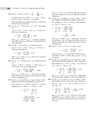
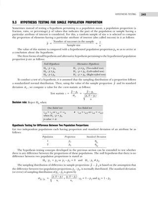
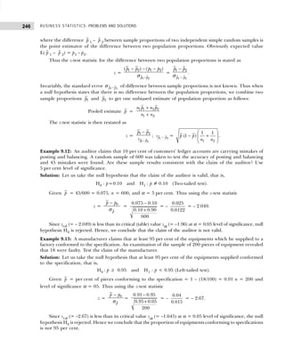
![247
HYPOTHESIS TESTING
Example 9.14: A company is considering two different television advertisements for promotion of a new
product. Management believes that advertisement A is more effective than advertisement B. Two test
market areas with virtually identical consumer characteristics are selected: advertisement A is used in one
area and advertisement B in the other area. In a random sample of 60 customers who saw advertisement
A, 18 had tried the product. In a random sample of 100 customers who saw advertisement B, 22 had tried
the product. Does this indicate that advertisement A is more effective than advertisement B, if a 5 per cent
level of significance is used? [Delhi Univ., MFC, 1996; MBA, 2000]
Solution: Let us take the null hypothesis that both advertisements are equally effective, that is,
H0 : p1 = p2 and H1 : p1 > p2 (Right-tailed test)
where p1 and p2 = proportion of customers who saw advertisement A and advertisement B respectively.
Given n1 = 60, 1
p = 18/60 = 0.30; n2 = 100, 2
p = 22/100 = 0.22 and level of significance α = 0.05.
Thus using the z-test statistic.
z =
1 2
1 2 1 2
( ) ( )
p p
p p p p
s −
− − −
=
1 2
1 2
p p
p p
s −
−
; p1 = p2
where sp p
1 2
− =
1 2
1 1
(1 )
p p
n n
− +
; q = 1 – p
=
1 1
0.25 0.75
60 100
× +
=
160
0.1875
600
= 0.0707;
p =
1 1 2 2
1 2
n p n p
n n
+
+
=
( ) ( )
60 18 /60 100 22/100
60 100
+
+
=
18 22
160
+
=
40
160
= 0.25.
Substituting values in z-test statistic, we have
z =
0.30 0.22
0.0707
−
=
0.08
0.0707
= 1.131
Since zcal =1.131 is less than its critical value zα = 1.645 at α = 0.05 level of significance, the null
hypothesis, H0, is accepted. Hence we conclude that there is no significant difference in the effectiveness
of the two advertisements.
Example 9.15: In a simple random sample of 600 men taken from a big city, 400 are found to be
smokers. In another simple random sample of 900 men taken from another city 450 are smokers. Do the
data indicate that there is a significant difference in the habit of smoking in the two cities?
[Raj Univ., M.Com., 1998; Punjab Univ., M.Com., 1996]
Solution: Let us take the null hypothesis that there is no significant difference in the habit of smoking in
the two cities, that is,
H0 : p1 = p2 and H1 : p1 ≠ p2 (Two-tailed test)
where p1 and p2 = proportion of men found to be smokers in the two cities.
Given n1 = 600, 1
p = 400/600 = 0.667; n2 = 900, 2
p = 450/900 = 0.50 and level of significance α
= 0.05. Thus, using the z-test statistic
z =
1 2
1 2 1 2
( ) ( )
p p
p p p p
s −
− − −
=
1 2
1 2
p p
p p
s −
−
; p1 = p2
where 1 2
p p
s − =
1 2
1 1
(1 )
p p
n n
− +
; q = 1 – p
=
1 1
0.567 0.433
600 900
× +
= 0.245 (0.002) = 0.026;](https://image.slidesharecdn.com/businessstatisticsproblemsandsolutions-230910073954-6d42a210/85/Business-Statistics_-Problems-and-Solutions-pdf-261-320.jpg)
![BUSINESS STATISTICS: PROBLEMS AND SOLUTIONS
248
p = 1 1 2 2
1 2
n p n p
n n
+
+
=
600 (400/600) 900 (450/900)
600 900
+
+
=
400 450
1500
+
=
850
1500
= 0.567.
Substituting values in z-test statistic, we have
z =
0.667 0.500
0.026
−
=
0 167
0 026
.
.
= 6.423.
Since zcal = 6.423 is greater than its critical value zα/2 = 2.58, at α/2 = 0.025 level of significance, the
null hypothesis, H0, is rejected. Hence we conclude that there is a significant difference in the habit of
smoking in two cities.
9.4 HYPOTHESIS TESTING FOR A BINOMIAL PROPORTION
The z-test statistic for determining the magnitude of the difference between the number of successes in a
sample and the hypothesized (expected) number of successes in the population is given by
z =
Sample estimate – Expected value
Standard error of estimate
=
x np
npq
−
.
Recalling from previous discussion that although sampling distribution of the number of successes in
the sample follows a binomial distribution having its mean µ = np and standard deviation npq , the normal
distribution provides a good approximation to the binomial distribution provided the sample size is large,
that is, both np ≥ 5 and n (1 – p) ≥ 5.
Example 9.16: Suppose the production manager implements a newly developed sealing system for boxes.
He takes a random sample of 200 boxes from the daily output and finds that 12 need rework. He is
interested to determine whether the new sealing system has increased defective packages below 10 per cent.
Use 1 per cent level of significance.
Solution: Let us state the null and alternative hypotheses as follows:
H0 : p ≥ 0.10 and H1 : p < 0.10 (Left-tailed test)
Given n = 200, p = 0.10, and level of significance α = 0.01. Applying the z-test statistic
z =
x np
npq
−
=
12 200 (0.10)
200 (0.10) (0.90)
−
=
12 20
18
−
= –1.885.
Since zcal (–1.885) is more than its critical value zα = – 2.33 for one-tailed test at α = 0.01 level of
significance, the null hypothesis, H0, is accepted. Hence we conclude that the proportion of defective
packages with the new sealing system is more than 10 per cent.
Example 9.17: In 324 throws of a six-faced dice, odd points appeared 180 times. Would you say that the
dice is fair at 5 per cent level of significance? [MD Univ., M.Com., 1997]
Solution: Let us take the hypothesis that the dice is fair, that is,
H0 : p = 162/324 = 0.5 and H1 : p ≠ 0.5 (Two-tailed test)
Given n = 324, p = q = 0.5 (i.e., 162 odd or even points out of 324 throws). Applying the z-test statistic:
z =
x np
npq
−
=
180 162
324 0.5 0.5
−
× ×
=
18
9
= 2.
Since zcal = 2 is more than its critical value zα/2 = 1.96 at α/2 = 0.025 significance level, the null
hypothesis H0 is rejected. Hence we conclude that the dice is not fair.](https://image.slidesharecdn.com/businessstatisticsproblemsandsolutions-230910073954-6d42a210/85/Business-Statistics_-Problems-and-Solutions-pdf-262-320.jpg)
![249
HYPOTHESIS TESTING
Example 9.18: Of those women who are diagnosed to have early-stage breast cancer, one-third eventually
die of the disease. Suppose an NGO launches a screening programme to provide for the early detection
of breast cancer and to increase the survival rate of those diagnosed to have the disease. A random sample
of 200 women was selected from among those who were periodically screened and who were diagnosed to
have the disease. If 164 women in the sample of 200 survive the disease, can screening programme be
considered effective? Test using α=0.01 level of significance and explain the conclusions from your test.
Solution: Let us take the null hypothesis that the screening programme was effective, that is,
H0: p = 1 – (1/3) = 2/3 and H1: p > 2/3.
Given n = 200, p = 2/3, q = 1/3 and α = 0.05. Applying the z-test statistic,
z =
x np
npq
−
=
164 200 (2/ 3)
200 (2/ 3)(1/ 3)
− ×
×
=
164 133.34
44.45
−
=
30.66
6.66
= 4.60.
Since zcal = 4.60 is greater than its critical value zα = 2.33 at α = 0.01 significance level, the null
hypothesis H0 is rejected. Hence we conclude that the screening programme was not effective.
S e l f-P r a c t i c e P r o b l e m s 9B
9.11 A company manufacturing a certain type of breakfast
cereal claims that 60 per cent of all housewives prefer
that type to any other. A random sample of 300
housewives contains 165 who do prefer that type. At
5 per cent level of significance, test the claim of the
company.
9.12 An auditor claims that 10 per cent of a company’s
invoices are incorrect. To test this claim a random
sample of 200 invoices is checked and 24 are found to
be incorrect. At 1 per cent significance level, test
whether the auditor’s claim is supported by the sample
evidence.
9.13 A sales clerk in the department store claims that
60 per cent of the shoppers entering the store leave
without making a purchase. A random sample of 50
shoppers showed that 35 of them left without buying
anything. Are these sample results consistent with the
claim of the sales clerk? Use a significance level of
0.05. [Delhi Univ., MBA, 1998, 2001]
9.14 A dice is thrown 49,152 times and of these 25,145
yielded either 4, 5, or 6. Is this consistent with the
hypothesis that the dice must be unbiased?
9.15 A coin is tossed 100 times under identical conditions
independently yielding 30 heads and 70 tails. Test at
1 per cent level of significance whether or not the coin
is unbiased. State clearly the null hypothesis and the
alternative hypothesis.
9.16 Before an increase in excise duty on tea, 400 people
out of a sample of 500 persons were found to be tea
drinkers. After an increase in the duty, 400 persons
were known to be tea drinkers in a sample of 600
people. Do you think that there has been a significant
decrease in the consumption of tea after the increase
in the excise duty?
[Delhi Univ., M.Com., 1998; MBA, 2000]
9.17 In a random sample of 1000 persons from UP 510
were found to be consumers of cigarattes. In another
sample of 800 persons from Rajasthan, 480 were
found to be consumers of cigarattes. Do the data reveal
a significant difference between UP and Rajasthan so
far as the proportion of consumers of cigarattes is
concerned? [MC Univ., M.Com., 1996]
9.18 In a random sample of 500 persons belonging to
urban areas, 200 are found to be using public
transport. In another sample of 400 persons belonging
to rural area 200 are found to be using public transport.
Do the data reveal a significant difference between
urban and rural areas so far as the proportion of
commuters of public transport is concerned (use
1 per cent level of significance).
[Bharathidasan Univ., M.Com., 1998]
9.19 A machine puts out 10 defective units in a sample of
200 units. After the machine is overhauled it puts out
4 defective units in a sample of 100 units. Has the
machine been improved?
[Madras Univ., M.Com., 1996]
9.20 500 units from a factory are inspected and 12 are
found to be defective, 800 units from another factory
are inspected and 12 are found to be defective. Can it
be concluded that at 5 per cent level of significance
production at the second factory is better than in first
factory? [Kurukshetra Univ., MBA, 1996;
Delhi Univ., MBA, 2002]
9.21 In a hospital 480 female and 520 male babies were
born in a week. Do these figures confirm the hypothesis
that females and males are born in equal number?
[Madras Univ., M.Com., 1997]
9.22 A wholesaler of eggs claims that only 4 per cent of the
eggs supplied by him are defective. A random sample
of 600 eggs contained 36 defectives. Test the claim of
the wholesaler. [IGNOU, 1997]](https://image.slidesharecdn.com/businessstatisticsproblemsandsolutions-230910073954-6d42a210/85/Business-Statistics_-Problems-and-Solutions-pdf-263-320.jpg)
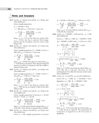
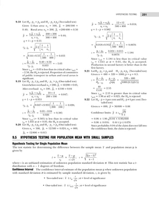
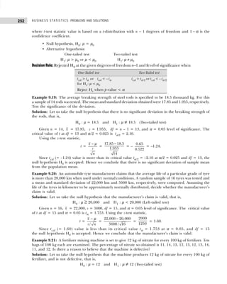
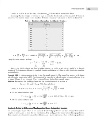
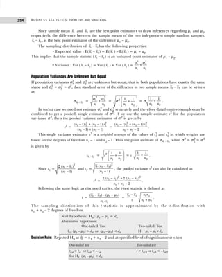
![255
HYPOTHESIS TESTING
Confidence Interval: The confidence interval estimate of the difference between populations means for
small samples of size n1 < 30 and/or n2 < 30 with unknown σ1 and σ2 estimated by s1 and s2 is given by
( 1 2
x x
− ) ± tα/2 1 2
x x
s −
where tα /2 is the critical value of t. The value of tα /2 depends on the t-distribution with
n1 + n2 – 2 degrees of freedom and confidence coefficient 1 – α.
Population Variances Are Unknown and Unequal
When two population variances are not equal, we may estimate the standard error 1 2
x x
−
σ of the statistic
( 1 2
x x
− ) by sample variances s1
2
and s2
2
in place of σ1
2
and σ2
2
. Thus an estimate of standard error of 1 2
x x
−
is given by
−
1 2
x x
s =
2
2
2
1
1 2
s
s
n n
+ .
The sampling distribution of a t-test statistic t =
1 2
1 2 1 2
( ) ( )
x x
x x
s −
− − −
µ µ
=
1 2
1 2
x x
x x
s −
−
is approximated by t-distribution with degrees of freedom given by
Degrees of freedom (df) =
2 2 2
1 1 2 2
2 2
2 2
2 2
1 1
1 2
[ / / ]
( / )
( / )
1 1
s n s n
s n
s n
n n
+
+
− −
.
The number of degrees of freedom in this case is less than that obtained in Case 1 above.
Example 9.23: In a test given to two groups of students, the marks obtained are as follows:
First group : 18 20 36 50 49 36 34 49 41
Second group : 29 28 26 35 30 44 46
Examine the significance of the difference between the arithmetic mean of the marks secured by the
students of the above two groups. [Madras Univ., M.Com., 1997; MD Univ., M.Com., 1998]
Solution: Let us take the null hypothesis that there is no significant difference in arithmetic mean of the
marks secured by students of the two groups, that is,
H0 : µ1 – µ2 = 0 or µ1 = µ2 and H1 : µ1 ≠ µ2 (Two-tailed test).
Since sample size in both the cases is small and sample variances are not known, apply t-test statistic
to test the null hypothesis
t =
1 2 1 2
1 2
x x n n
s n n
−
+
.
Calculations of sample means 1
x , 2
x and pooled sample standard deviations are shown in Table 9.2.
Table 9.2 Calculation for x1 , x2 and s
First Group x1 – 1
x (x1 – 1
x )2
Second Group x2 – 2
x (x2 – 2
x )2
x1 = x1 – 37 x2 = x2 – 34
18 –19 361 29 –5 25
20 –17 389 28 –6 36
36 –1 1 26 –8 64
50 13 169 35 1 1
49 12 144 30 –4 16
36 –1 1 44 10 100
34 –3 9 46 12 144
49 12 144
41 4 16
333 0 1,234 238 0 386](https://image.slidesharecdn.com/businessstatisticsproblemsandsolutions-230910073954-6d42a210/85/Business-Statistics_-Problems-and-Solutions-pdf-269-320.jpg)
![BUSINESS STATISTICS: PROBLEMS AND SOLUTIONS
256
1
x = 1
1
x
n
Σ
=
333
9
= 37 and 2
x =
2
2
x
n
Σ
=
238
7
= 34
s =
2 2
1 1 2 2
1 2
( ) ( )
2
x x x x
n n
Σ − + Σ −
+ −
=
1234 386
9 7 2
+
+ −
= 9.76
Substituting values in the t-test statistic, we get
t = 1 2 1 2
1 2
x x n n
s n n
−
+
=
37 34 9 7
10.76 9 7
− ×
+
=
3
10.46
×1.984 = 0.551.
Degrees of freedom, df = n1 + n2 – 2 = 9 + 7 – 2 = 14.
Since at α = 0.05 and df = 14, the calculated value tcal (= 0.551) is less than its critical value tα/2 =
2.14, the null hypothesis H0 is accepted. Hence we conclude that the mean marks obtained by the students
of two groups do not differ significantly.
Example 9.24: The mean life of a sample of 10 electric light bulbs was found to be 1456 hours with
standard deviation of 423 hours. A second sample of 17 bulbs chosen from a different batch showed a
mean life of 1280 hours with standard deviation of 398 hours. Is there a significant difference between
the means of the two batches. [Delhi Univ., M.Com., 1997]
Solution: Let us take the null hypothesis that there is no significant difference between the mean life of
electric bulbs of two batches, that is,
H0 : µ1 = µ2 and H1 : µ1 ≠ µ2 (Two-tailed test)
Given n1 = 10, 1
x = 1456, s1 = 423; n2 = 17, 2
x = 1280, s2 = 398 and α = 0.05. Thus,
Pooled standard deviation, s =
2 2
1 1 2 2
1 2
( 1) ( 1)
2
n s n s
n n
− + −
+ −
=
2 2
9 (423) 16 (398)
10 17 2
+
+ −
=
16,10,361 25,34,464
25
+
= 1,65,793 = 407.18.
Applying the t-test, we have
t = 1 2 1 2
1 2
x x n n
s n n
−
+
=
1456 1280 10 17
407.18 10 17
− ×
+
=
176
407.18
×2.51 = 1.085.
Since the calculated value tcal = 1.085 is less than its critical value tα/2 = 2.06 at df = 25 and α = 0.05 level
of significance, the null hypothesis is accepted. Hence we conclude that the mean life of electric bulbs of two
batches does not differ significantly.
Example 9.25: The manager of a courier service believes that packets delivered at the end of the month
are heavier than those delivered early in the month. As an experiment, he weighed a random sample of
20 packets at the beginning of the month. He found that the mean weight was 5.25 kgs with a standard
deviation of 1.20 kgs. Ten packets randomly selected at the end of the month had a mean weight of 4.96
kgs and a standard deviation of 1.15 kgs. At the 0.05 significance level, can it be concluded that the
packets delivered at the end of the month weigh more?
Solution: Let us take the null hypothesis that the mean weight of packets delivered at the end of the
month is more than the mean weight of packets delivered at the beginning of the month, that is,
H0 : µE ≥ µB and H1 : µE < µB
Given n1 = 20, 1
x = 5.25, s1 = 1.20 and n2 = 10, 2
x = 4.96, s2 = 1.15. Thus,
Pooled standard deviation, s =
( ) ( )
2 2
1 1 2 2
1 2
1 1
2
n s n s
n n
− + −
+ −
=
( ) ( )
2 2
19 5.25 9 4.96
20 10 2
× +
+ −
=
19 27.56 9 24.60
28
× + ×
= 26.60 = 5.16.](https://image.slidesharecdn.com/businessstatisticsproblemsandsolutions-230910073954-6d42a210/85/Business-Statistics_-Problems-and-Solutions-pdf-270-320.jpg)
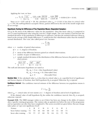
![BUSINESS STATISTICS: PROBLEMS AND SOLUTIONS
258
Solution: Let us take the null hypothesis that there is no change that has taken place after the training,
that is,
H0 : µd = 0 and H1 : µd ≠ 0 (Two-tailed test)
The ‘changes’ are computed as shown in Table 9.3 and then a t-test is carried out on these differences
as shown below.
d =
Σ d
n
=
−45
9
= –5 and
sd =
2 2
( )
1 ( 1)
d d
n n n
Σ Σ
−
− −
=
2
( 45)
903
8 9 8
−
−
×
= 112.87 28.13
− = 9.21.
Applying the t-test statistic, we have
t =
/
d
d
d
s n
− µ
=
5 0
9.21/ 9
− −
= –
5
3.07
= –1.63.
Since the calculated value tcal = –1.63 is more than its critical value tα/2 = – 2.31, at df = 8 and α/2 =
0.025, the null hypothesis is accepted. Hence, we conclude that there is no change in the ability of
trainees after the training.
Example 9.27: 12 students were given intensive coaching and 5 tests were conducted in a month. The
scores of tests 1 and 5 are given below.
No. of students : 51 52 53 54 55 56 57 58 59 10 11 12
Marks in 1st test : 50 42 51 26 35 42 60 41 70 55 62 38
Marks in 5th test : 62 40 61 35 30 52 68 51 84 63 72 50
Do the data indicate any improvement in the scores obtained in tests 1 and 5?
[Punjab Univ., M.Com., 1999]
Solution: Let us take the hypothesis that there is no improvement in the scores obtained in the first and
fifth tests, that is,
H0 : µd = 0 and H1 : µd ≠ 0 (Two-tailed test).
The ‘changes’ are calculated as shown in Table 9.4 and then t-test is carried out on these differences
as shown below:
d =
d
n
Σ
=
96
12
= 8 and sd =
2 2
( )
1 ( 1)
d d
n n n
Σ Σ
−
− −
=
2
1122 (96)
11 12 11
−
×
= 5.673.
Table 9.3 Calculations of ‘Changes’
Trainee Before After Difference d2
Training Training in Scores, d
A 75 70 5 25
B 70 77 7 49
C 46 57 –11 121
D 68 60 8 64
E 68 79 –11 121
F 43 64 –21 441
G 55 55 0 0
H 68 77 –9 81
I 77 76 1 1
–45 903](https://image.slidesharecdn.com/businessstatisticsproblemsandsolutions-230910073954-6d42a210/85/Business-Statistics_-Problems-and-Solutions-pdf-272-320.jpg)
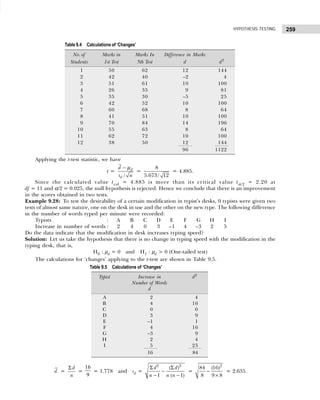
![BUSINESS STATISTICS: PROBLEMS AND SOLUTIONS
260
Applying the t-test statistic, we have
t =
/
d
d
d
s n
− µ
=
1.778
2.625/ 9
= 2.025.
Since the calculated value tcal = 2.025 is less then its critical value tα = 2.306 at df = 8 and α = 0.05
significance level, the null hypothesis is accepted. Hence we conclude that there is no change in typing
speed with the modification in the desk.
S e l f-P r a c t i c e P r o b l e m s 9C
9.23 Ten oil tins are taken at random from an automatic
filling machine. The mean weight of the tins is 15.8 kg
and the standard deviation is 0.50 kg. Does the sample
mean differ significantly from the intended weight of
16 kg? [Delhi Univ., MBA,1998]
9.24 Nine items of a sample had the following values: 45,
47, 50, 52, 48 47, 49, 53, and 50. The mean is 49 and
the sum of the square of the deviation from mean is
52. Can this sample be regarded as taken from the
population having 47 as mean? Also obtain 95 per cent
and 99 per cent confidence limits of the population
mean. [Delhi Univ., MBA,1996]
9.25 The electric bulbs of 10 random samples from a large
consignment gave the following data:
Item Life in ’000 hours
1 4.2
2 4.6
3 3.9
4 4.1
5 5.2
6 3.8
7 3.9
8 4.3
9 4.4
10 5.6
Can we accept the hypothesis that the average lifeime
of the bulbs is 4000 hours.
[Madras Univ., M.Com.,1998]
9.26 A random sample of size 16 has 53 as mean. The sum
of the squares of the deviations taken from mean is
135. Can this sample be regarded as taken from the
population having 56 as mean? Obtain 95 per cent
and 99 per cent confidence limits of the mean of the
population. [Madras Univ., M.Com.,1998]
9.27 A drug manufacturer has installed a machine which
automatically fills 5 g of drug in each phial. A random
sample of fills was taken and it was found to contain
5.02 g on an average in a phial. The standard deviation
of the sample was 0.002 g. Test at 5% level of
significance if the adjustment in the machine is in
order. [Delhi Univ., MBA,1999]
9.28 Two salesmen A and B are working in a certain district.
From a sample survey conducted by the Head Office,
the following results were obtained. State whether
there is any significant difference in the average sales
between the two salesmen.
Salesman
A B
No. of samples : 20 18
Average sales (Rs. in thousand) : 170 205
Standard deviation (Rs. in thousand) : 20 25
[Delhi Univ., MBA, 1994;
Kumaon Univ., MBA, 2000]
9.29 The means of two random samples of sizes 9 and 7
are 196.42 and 198.82, respectively. The sum of the
squares of the deviations from the mean are 26.94
and 18.73, respectively. Can the sample be considered
to have been drawn from the same normal population?
[Delhi Univ., M.Com., 1996]
9.30 Strength tests carried out on samples of two yarns
spurn to the same count gave the following results:
Sample Sample Sample
Size Mean Variance
Yarn A 4 52 42
Yarn B 9 42 56
The strength is expressed in kg. Is the difference in
mean strengths significant of the real difference in the
mean strengths of the sources from which the samples
are drawn? [Delhi Univ., MBA, 2000]
9.31 A random sample of 12 families in one city showed an
average monthly food expenditure of Rs. 1380 with a
standard deviation of Rs. 100 and a random sample of
15 families in another city showed an average monthly
food expenditure of Rs. 1320 with a standard deviation
of Rs. 120. Test whether the difference between the
two means is significant at α = 0.01 level of significance
of α = 0.01. [AIMA Diploma in Mgmt., 1987;
Delhi Univ., MBA, 1991]](https://image.slidesharecdn.com/businessstatisticsproblemsandsolutions-230910073954-6d42a210/85/Business-Statistics_-Problems-and-Solutions-pdf-274-320.jpg)
![261
HYPOTHESIS TESTING
9.32 You are given the following data about the life of two
brands of bulbs:
Mean Life Standard Sample
Deviation Size
Brand A 2000 hours 250 hours 12
Brand B 2230 hours 300 hours 15
Do you think there is a significant difference in the
quality of the two brands of bulbs?
[Delhi Univ., MBA, 1996]
9.33 Eight students were given a test in statistics, and after
one month’s coaching, they were given another test
of the similar nature. The following table gives the
increase in their marks in the second test over the
first:
Roll No. Increase in Marks
1 2
2 –2
3 6
4 –8
5 12
6 5
7 –7
8 2
Do the marks indicate that the students have gained
from the coaching?
9.34 An IQ test was administered to 5 persons before and
after they were trained. The results are given below:
Candidate I II III IV V
IQ before training : 110 120 123 132 125
IQ after training : 120 118 .25 136 121
Test whether there is any change in IQ level after the
training programme. [Delhi Univ., M.Com., 1998]
9.35 Eleven sales executive trainees are assigned selling
jobs right after their recruitment. After a fortnight
they are withdrawn from their field duties and given a
month’s training for executive sales. Sales executed
by them in thousands of rupees before and after the
training, in the same period, are listed below:
Sales Before Training Sales After Training
23 24
20 19
19 21
21 18
18 20
20 22
18 20
17 20
23 23
16 20
19 27
Do these data indicate that the training has contributed
to their performance? [Delhi Univ., M.Com., 1999]
Hints and Answers
9.23 Let H0 : µ = 16 and H1 : µ ≠ 16 (Two-tailed test)
Given n = 10, x = 15.8, s = 0.50. Using t-test
t =
/
x
s n
− µ
=
15.8 16
0.50/ 10
−
= – 1.25
Since tcal = –1.25 > critical value tα/2 = – 2.262, at df
= 9 and α/2 = 0.025, the null hypothesis is accepted.
9.24 Let H0 : µ = 27 and H1 : µ ≠ 47 (Two-tailed test)
Given x = 49, Σ(x – x )2
= 52, n = 9, and
s =
2
( )
( 1)
x x
n
Σ −
−
=
52
8
= 2.55.
t =
/
x
s n
− µ
=
49 47
2.55/ 9
−
= 2.35
Since tcal = 2.35 > critical value tα/2 = 2.31 at α/2 =
0.025, df = 8, the null hypothesis is rejected.
9.25 Let H0 : µ = 4,000 and H1 : µ ≠ 4000 (Two-tailed test)
s =
2
( )
( 1)
x x
n
Σ −
−
=
3.12
9
= 0.589 and
x = /
x n
∑ = 44/10 = 4.4 (in Rs. 000’s).
t =
/
x
s n
− µ
=
4.4 4
0.589 / 10
−
=
0.4
0.186
= 2.150
Since tcal = 2.150 < critical value tα/2 = 2.62 at
α/2 = 0.025 and df = n – 1 = 9, the null hypothesis is
accepted.
9.26 Let H0 : µ = 56 and H1 : µ ≠ 46 (Two-tailed test)
Given n = 16, x = 53, and Σ(x – x )2
= 135. Thus,
s =
2
( )
( 1)
x x
n
Σ −
−
=
135
15
= 3
Applying t-test, t =
/
x
s n
− µ
=
53 56
3/ 16
−
= –4
Since tcal = –4 < critical value tα/2 = –2.13 at
α/2 = 0.025, df = 15, the null hypothesis is rejected.
9.27 Let H0 : µ = 5 and H1 : µ ≠ 5 (Two-tailed test)
Given n = 10, x = 5.02, and s = 0.002.](https://image.slidesharecdn.com/businessstatisticsproblemsandsolutions-230910073954-6d42a210/85/Business-Statistics_-Problems-and-Solutions-pdf-275-320.jpg)
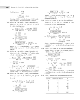
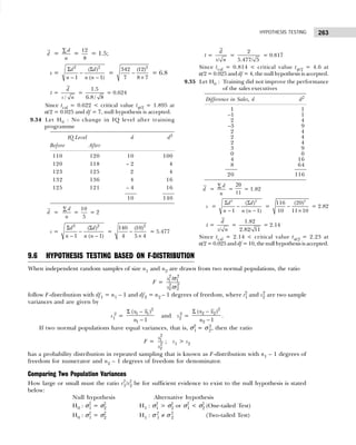
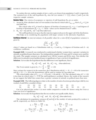
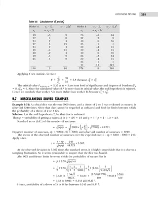
![BUSINESS STATISTICS: PROBLEMS AND SOLUTIONS
266
Example 9.32: A coin is tossed 400 times and it turns up head 216 times. Discuss whether the coin may
be an unbiased one and explain briefly the theoretical principles you would use for this purpose.
Solution: Let the hypothesis be that the coin is unbiased. Then the chance of turning up head in a toss p
= 1/2 and q = 1 – p = 1 – (1/2) = 1/2.
Expected number of heads in 400 tosses: np = 400 × (1/2) = 200 and observed number of heads in 400
tosses is 216. Thus, the excess of the observed number of heads in 400 tosses over the expected number:
216 – 200 = 15 = 16.
The standard error of the number of heads
= [ ]
× ×
( ) = 400 (1/2) (1/2) = (100) =10
npq .
Apply z-test, z =
− 16
=
10
x np
npq
= 1.6.
As | z | < 2, the difference between the observed and expected number of heads is not significant, that is,
deviations likely to appear due to simple sampling fluctuations. So we conclude that the coin was perhaps
an unbiased one.
Example 9.33: 10 dice are thrown 300 times each and a throw of an odd numbers reckoned as a success.
Are the dice unbiased if 1650 throws of odd numbers have been obtained?
Solution: Let the hypothesis be that the dice are unbiased. The chance of getting an odd number, viz. 1,
3, or 5 with one dice in a throw p = 3/6 = 1/2 and p = 1 – p = 1 – (1/2) = 1/2. The total number of throws
10 × 300 = 300. Expected number of successes, np = 3000 × 1/2 = 1500, and observed number of
successes: 1650
The excess of the observed number of successes over the expected number of successes 1650 – 1500
= 150.
The standard error of the number of successes
=
1 1
( ) 3000 (750)
2 2
npq
= × × =
.
Apply z-test, z =
− 150
= = 5.47
750
x np
npq
.
As | z | > 3, the difference between the observed and the expected number of successes is highly significant,
that is, deviation is most likely to have occurred due to fluctuations in sampling and the dice are unbiased.
Example 9.34: A certain stimulus administered to each of 12 patients resulted in the following increases
of blood pressures: 5, 2, 8, –1, 3, 0, 6, –2, 1, 5, 0, 4. Can it be concluded that the simulus will be, in
general, accompanied by an increase in blood pressure?
Solution: Let us take the hypothesis that simulus accompanied an increase in blood pressure.
Let the assumed mean A be 2. Calculating mean x and standard deviation σ of the sample as follows:
x f d=x – A fd d2
fd2
–2 1 –4 –4 16 16
–1 1 –3 –3 9 9
0 2 –2 –4 4 8
1 1 –1 –1 1 1
2 ← A 1 0 0 0 0
3 1 1 1 1 1
4 1 2 2 4 4
5 2 3 6 9 18
6 1 4 4 16 16
8 1 6 6 36 36
12 7 109](https://image.slidesharecdn.com/businessstatisticsproblemsandsolutions-230910073954-6d42a210/85/Business-Statistics_-Problems-and-Solutions-pdf-280-320.jpg)
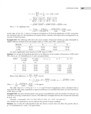
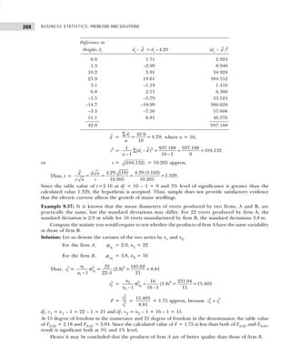
![269
HYPOTHESIS TESTING
Example 9.38: Two gauge operators are tested for precision in making measurements. One operator
completes a set of 26 readings with a standard deviation of 1.34 and the other does 34 readings with a
standard deviation of 0.98. What is the level of significance of this difference? Give that for v1 = 25 and
v2 = 33, z0.05 = 0.366 and z0.01 = 0.432.
Solution: Let the variates of the two series be denoted by x1 and x2. Then σx1
= 1.34, n1 = 26 and
σx2
= 0.98, n2 = 34. Then
s1 =
1
1
1
26
= 1.34
1 25
x
n
n
×
−
σ
and s2 = 2
2
2
34
= 0.98
1 33
x
n
n
×
−
σ .
z =
3
2
1 1 1
10 10
2
2 2
2
1
log 1.1513 log 2.3026 log
2
e
s s s
s s
s
= =
=
26 33 1
2.3026 log 1.34
25 34 0.98
× × ×
=
× ×
1/2
26 33 1.34
2.3026 log
25 34 0.98
= 2.3026
1
{log 26 log 33 log 25 log 34} log1.34 log 0.98
2
+ − − + −
= 1.1513[1.4150 + 1.5185 – 1.3979 – 1.5315] + 2.3026 [0‘1271 – 1.9912 ]
= (1.1513) [0.0041] + (2.3026) [0.1359]
= (1.1513) [0.0041 + 0.2718] = (1.1513) × (0.2759) = 0.318.
As the calculated value of z = 0.318 is slightly greater than z0.05 = 0.366 and less than z0.01 = 0.432 the
difference between the standard deviations is significant at 5% level and not significant at 1% level.
Example 9.39: Show how you would use Student’s t-test and Fisher’s z-test to decide whether the two sets
of observations: 17, 27, 18, 25, 27, 29, 27, 23, 17 and 16, 16, 20, 16, 20, 17, 15, 21 indicate samples from
the same universe.
Solution: Let the variates of two sets of observations be denoted by x1 and x2. Then mean and standard
deviation of the two series are calculated as given below:
I Set of Observations II Set of Observations
x1 x1 – d1 = x1 – 23 (x1 – d1)2
x2
x2 – d2 = x2 – 16 (x2 – d2)2
17 –6 36 16 0 0
27 4 16 16 0 0
18 –5 25 20 4 16
25 2 4 16 ← 2
d 0 0
27 4 16 20 4 16
29 6 36 17 1 1
27 4 16 15 –1 1
23 ← 1
d 0 0 21 5 25
17 –6 36
210 3 185 141 13 59
where n1 = 9 and n2 = 8. Thus,](https://image.slidesharecdn.com/businessstatisticsproblemsandsolutions-230910073954-6d42a210/85/Business-Statistics_-Problems-and-Solutions-pdf-283-320.jpg)
![BUSINESS STATISTICS: PROBLEMS AND SOLUTIONS
270
1
x =
∑
∑ 2
1
2
1 2
210 141
= =23.333, and = = =17.625
9 8
x
x
x
n n
.
Let us assume the means of x1 and x2 series as 1
d = 23, 2
d = 16. Then
2
1
s =
∑ − ∑ −
−
− −
2 2 2
1 1 1 1
1 1 1
( ) ( ) (3)
185
= –
1 ( 1) 8 9 (8)
x d x d
n n n
= 185 1 184
8 8 8
− = = 23
and 2
2
s =
∑ − ∑ −
− −
− −
2 2 2
2 2 2 2
2 2 2
( ) ( ) (13)
59
=
1 ( 1) 7 8 (7)
x d x d
n n n
=
59 169 303
– = =5.411 approx.
7 56 56
Using z-test to find whether the population variances are the same, that is, σ1 = σ2
z =
2 2
1 1
10
2 2
2 2
1 23
log 1.1513 log 1.1513 log
2 5.411
e
s s
s s
= =
= 1.1513 [log 23 – log 5.411] = 1.1513 [1.3617 – 0.7333] = 0.724 approx.
At df, v1 = 8 and df, v2 = 7, z0.05 = 0.6576 and z0.01 = 0.9614.
Since calculated value of z = 0.724 is greater than z0.05 = 0.6576 and less than z0.01 = 0.9614, the
variance ratio is significant for 5% points and not significant for 1% points. For 1% level, the two population
variances are the same.
Using t-test to measure the significance of the difference between the population means. Let us take
the hyothesis that µ1 = µ2. Then
t =
( )
−
−
+
+
1 2 1 2
1 2
1 2
1 2
( ) ( )
=
( )
(1/ ) 1/
x x n n
x x
s n n
s n n
=
(23.333 17.625) (72)
(3.846) (17)
−
=
(5.708) (8.485) 48.432
3.054
(3.846) (4.123) 15.857
= = ,
where s2
=
2 2
1 1 2 2
1 2
( 1) ( 1)
2
n s n s
n n
− + −
+ −
=
(9 1) (23) (8 1) (5.411) 184 37.877
9 8 2 15
− + − +
=
+ −
= 221.877
=14.729 approx.
(15)
or s = 14.792 3.846
=
df, v = n1 +n2 – 2 = 9+8 – 2 = 15, and t0.05 = 2.131 and t0.01 = 2.947.
As the calculated value of t = 3.054 is greater than both the table values of t, the difference between
the population means is significant. Hence the two samples do not belong to the same population.
Example 9.40: In a hospital 480 female and 520 males babies were born in a week. Do these figures
confirm the hypothesis that males and females are born in equal number? [Madras Univ, M.Com., 2000]
Solution: Let us take the hypothesis that male and female babies are born in equal number, that is, p = 1/2.
Calculating standard error as follows:
Standard error, σ = = 1000×0.5×0.5 =15.81
npq .
Difference between observed and expected number of female babies: 520 – 500 = 20.
Difference
S.E.
=
20
=1.265
15.81
.
Since the difference is less than 1.96 σ at 5% level of significance, it can be concluded that the male
and females babies are born in equal number.](https://image.slidesharecdn.com/businessstatisticsproblemsandsolutions-230910073954-6d42a210/85/Business-Statistics_-Problems-and-Solutions-pdf-284-320.jpg)
![271
HYPOTHESIS TESTING
Example 9.41: In a random sample of 1000 persons from U.P. 510 were found to be consumers of
cigrattes. In another sample of 800 persons from Rajasthan, 480 were found to be consumes of cigarattes.
Does the data reveal a significant difference between U.P. and Rajasthan so far as the production of
comsumers of cigaratters is concerned? [MD Univ., M.Com., 2005]
Solution: Let us take the hypothesis that there is no signigicant difference between U.P. and Rajasthan so
far as the proportion of consumers of cigatetters is concerned. Calculating standard error of difference of
proportions as follows:
Standard error, σp
1
–p
2
=
+
1 2
1 1
pq
n n
=
× +
1 1
0.55 0.45 =0.024
1000 800
where p1 =
510
= 0.51
1000
, and p2 =
480
= 0.60
800
p =
+ +
+ +
1 2
1 2
510 480
= =0.55
1000 800
x x
n n
, and q=1 – p=1 – 0.55=0.45.
Since z =
−
−
1 2
1 2
p p
p p
s
=
0.51 – 0.6
= 3.75
0.024
is more than 2.58 S.E. at 1% level of significance, the hypothesis is rejected. Hence, the data reveal a
significant difference between U.P. and Rajasthan so far as proportion of consumers for cigarattes is
concerned.
Example 9.42: A sample of 100 tyres is taken from a lot. The mean life of years is found to be 39,350 km.
with a standard deviation of 3260. Could the sample come from a population with mean life of 40,000
km? Establish 99% confidence limits within which the mean life of tyres is expected to lie.
[Delhi Univ., B.A. (Eco. H), 1996]
Solution: (a) Let us take the null hypothesis that there is no significant difference between the sample
mean and the hypothetical population mean. Calculating standard error of means as follows:
Standard error, σ x =
3260
= = 326
100
n
σ
.
Since z =
x
x − µ
σ
=
40,000 – 39,350 650
= =1.994
326 326
is less than 2.58 σ x at 1% level of significance the hypothesis is accepted and the difference could have
arisen due to fluctuation of sampling.
(b) 99% confidence limits: x ± 2.58 σ x = 39,350 ± 2.58 (326)
= 39,350 ± 841.08, i.e., 3858.92 ≤ x ≤ 40,191.08
Hence the mean life of tyres is expected to lie between 38,509 and 40,191.
Example 9.43: A man buys 50 electric bulbs of ‘Philips’ and 50 electric bulbs of ‘HMT’. He finds that
‘Philips’ bulbs have an average life of 1500 hours with a standard deviation of 60 hours and ‘HMT’ bulbs
have an average life of 1512 hours with a standard deviation of 80 hours. Is there a significant difference
in the mean life of the two makes of bulbs? [M.D. Univ., M.Com., 1998; Kumaon Univ., MBA, 2006]
Solution: Let us take the hypothesis that there is no significant difference in the mean life of the two
makes of bulbs. Calculating standard error of difference of means as follows:
Standard error, 1 2
x x
−
σ =
2
2
2
1
1 2
n n
+
σ
σ
=
+
+
2 2
3600 6400
(60) (80)
= = 200 =14.14
50 50 50
where σ1 = 60, n1 = 50, σ2 = 80, n2 = 50
Since z =
x
x − µ
σ
=
1512 – 1500
= 0.849
14.14
is less than 2.58 S.E. at 1% level of significances, the difference in the mean life of two makes is not
significant.](https://image.slidesharecdn.com/businessstatisticsproblemsandsolutions-230910073954-6d42a210/85/Business-Statistics_-Problems-and-Solutions-pdf-285-320.jpg)
![BUSINESS STATISTICS: PROBLEMS AND SOLUTIONS
272
Example 9.44: A simple sample of the height of 6400 Englishmen has a mean of 67.85 inches and a
standard deviation of 2.56 inches while a simple sample of heights of 1600 Austrians has a mean of 68.55
inches and standard deviation of 2.52 inches. Do the data indicate that the Austrians are on the average
taller than the Englishmen? Give reasons for your answer. [Kumaon Univ., MBA, 1999]
Solution: Let us take the typothesis that there is no significant difference in the mean height of Englishmen
and Austrians, that is, H0 : µ1 = µ2
Standard error, 1 2
x x
−
σ =
2
2
2
1
1 2
n n
+
σ
σ
= + +
2 2
(2.56) (2.52)
= 0.001 0.004 = 0.0707
6400 1600
where σ1 = 2.56, n1 = 6400, σ2 = 2.52, n2 = 1600.
Since z =
67.85 – 68.55 0.7
= =9.9
0.0707 0.0707
is more than S.E. at 1% level of significance, the hypothesis is rejected. Hence, the data indicates that the
Austrians are on the average taller than the Englishmen.
Example 9.45: In a sample of 1000, the mean is 17.5 and the standard deviation is 2.5. In another sample
of 800, the mean is 18 and standard deivation is 2.7. Assuming that the samples are independent, discuss
whether the two samples can have come from a population which has the same standard deviation.
[Saurashtra Univ. B.Com., 1997]
Solution: Let us take the hypothesis that there is no significant difference in the standard deviations of the
two samples. Calculating the standard error of difference between standard deviation of two samples as
follows:
Standard error, σσ1–σ2
=
σ
σ
+
2
2
2
1
1 2
n n
= + +
2 2
6.25
(2.5) (2.7) 7.29
=
2000 1600 2000 1600
= 0.0876
where σ1 = 2.5, n1 = 1000, σ2 = 2.7, n2 = 800.
Since z =
1 2
2 1
–
−
σ σ
σ σ
σ
=
2.7 – 2.5 0.2
= =2.283
0.0876 0.0876
is more than 1.96 S.E. at 5% level of significance, the hypothesis is rejected. Hence, the two samples have
not come from a population which has the same standard deviation.
Example 9.46: The mean produces of wheat of a sample of 100 fields is 200 lb. per acre with a standard
deviation of 10 lb. Another sample of 150 fields gives the mean at 220 with a standard deviation of 12 lb.
Assuming the standard deviation of the mean field at 1 lb. of the universe, find at 1% level of significance
if the two results are consistent. [Mangalore Univ., MBA, 1996]
Solution: Let us take the hypothesis that there is no significant difference in the standard deviations.
Calculating the standard error of difference between standard deviation of two sample as follows:
σσ1–σ2
=
2 2
1 2
1 1 (11) 1 1
=
2 2 100 150
n n
+ +
σ
= + +
60.5 60.5
= 0.605 0.403 =1.004
100 150
.
Difference between two standard deviations = (12 – 10) = 2 lb.
Since z =
1 2
2 1
−
−
σ σ
σ σ
σ
=
12–10
=1.992
1.004
is less than 2.58S.E. at 1% level of significance, the hypothesis is accepted and hence the two results may
be regarded as consistent.
Example 9.47: A random sample of size 16 has 53 as mean. The sum of the squares of the deviations taken
from mean is 135. Can this sample be regarded as taken from the population having 56 as mean? Obtain
95% and 99% confidence limits of the mean of the population. [Annamalai Univ., M.Com., 2003; CAFC, 2006]
Solution: Let us take the hypothesis that there is no signigicant difference between the sample mean and
hypothetical population mean. Applying t test,](https://image.slidesharecdn.com/businessstatisticsproblemsandsolutions-230910073954-6d42a210/85/Business-Statistics_-Problems-and-Solutions-pdf-286-320.jpg)
![273
HYPOTHESIS TESTING
t =
x
s n
− µ
=
− ×
53 56 3 4
= = 4
3
3/ 16
where x = 53, µ = 56, n = 16, Σ(x – x )2
= 135
s =
Σ −
−
( ) 135
= = 3
1 15
x x
n
; df(v) = 16 – 1 = 15. For v = 15, t0.05 = 2.13.
Since the calculated value of t is more than the table value, the hypothesis is rejected. Hence, the
sample has not come from a population having 56 as mean.
At 95% confidence limit of the population mean, we have
± 0.05
s
x t
n
= ± ×
3
53 2.13
16
= 53 ± 1.6 i.e. 51.4 ≤ x ≤ 54.6.
At 99% confidence limits of the population mean
± 0.05
s
x t
n
= ± ×
3
53 2.95
16
= ± ×
3
53 2.95
4
= 53 ± 2.212 = 50.788 to 55.212.
Example 9.48: The lifetime of electric bulbs for a random sample of 10 from a large consignment gave the
following data :
Item : 1 2 3 4 5 6 7 8 9 10
Life in ‘000 hours : 4.2 4.6 3.9 4.1 5.3 3.8 3.9 4.3 4.4 56
Can we accept the hypothesis that there is no significant difference in the sample mean and the
hypothetical population mean. [Univ., M.Com., 2005]
Solution: Let us take the hypothesis that there is no significant difference in the sample mean and the
hypothetical population mean. Applying the t-test,
t =
x
s n
− µ
=
− ×
4.4 4 0.4 3.162
10 = =2.148
0.589 0.589
.
Calculation of x and s
x (x – x ) (x – x )2
4.2 –0.2 0.04
4.6 0.2 0.04
3.9 –0.5 0.25
4.1 – 0.3 0.09
5.2 0.8 0.64
3.8 –0.6 0.36
3.9 –0.5 0.25
4.3 –0.1 0.01
4.4 0 0
5.6 1.2 1.44
44 3.12
where s =
Σ −
−
2
( ) 3.12
= =0.589
1 9
x x
n
; df, v = n – 1 = 10 – 1 = 9. For v = 9, t0.05 = 2.262.
Since the calculated value of t is less than its table value, the hypothesis is accepted, and hence average
lifetime of the bulbs could be 4000 hours.](https://image.slidesharecdn.com/businessstatisticsproblemsandsolutions-230910073954-6d42a210/85/Business-Statistics_-Problems-and-Solutions-pdf-287-320.jpg)
![BUSINESS STATISTICS: PROBLEMS AND SOLUTIONS
274
Example 9.49: For a random sample of 10 persons, fed on diet A, the increased weight in pounds in a
certain period was 10, 6, 16, 17, 13, 12, 8, 14, 15, 9.
For another random sample of 12 persons, fed on diet B, the increase in the same period was 7, 13,
22, 15, 12, 14, 18, 8, 21, 23, 10, 17. Test whether diets A and B differ significantly as regards their effect
on increase in weight. Given the following:
Degrees of freedom : 19 20 21 22 23
Value of t at 5% level : 2.09 2.09 2.08 2.07 2.07
[M.D. Univ., 2002]
Solution: Let us take the null hypothesis that diet A and B do not differ significantly with regard to their
effect on increase in weight. Apply t-test,
t =
− − ×
+ +
2 1 2
1 2
12 15 10 12 3
= = =1.51
4.66 12 12 4.66
x x n n
s n n
.
Calculating the required values as shown below :
Persons on Diet A Persons on Diet B
Increase in Deviations (x1 – 1
x )2
Increase in Deviations (x2 – 2
x )2
Weight from Mean 12 Weight from Actual
Mean 15
x1 (x1 – 1
x ) x2 (x2 – 2
x )
10 –2 4 7 –8 64
6 –6 36 13 –2 4
16 4 16 22 7 49
17 5 25 15 0 0
13 1 1 12 –3 9
12 0 0 14 –1 1
8 –4 16 18 3 9
14 2 4 8 –7 49
15 3 9 21 6 36
9 –3 9 23 8 64
10 –5 25
17 2 4
120 0 120 180 0 314
Mean increase in weight of 10 persons fed on diet A
1
x =
Σ 1
1
120
= =12 pounds
10
x
n
Mean increase in weight of 12 persons fed on diet B
2
x =
Σ 1
2
180
= =15 pounds
12
x
n
and Pooled standard deviation, s =
Σ − + Σ −
+ −
2
1 1 2 2
1 2
( ) ( )
2
x x x x
n n
=
+
+ −
120 314 434
= = 4.66
10 12 2 20
where df, v = n1 + n2 – 2 = 10 + 12 – 2 = 20.
For df, v = 20, the table value of t at 5 per cent level is 2.09. The calculated value of t is less than its
table value and hence the experiment provides no evidence against the hypothesis. Hence diet A and B do
not differ significantly with respect to their effect on increase in weight.](https://image.slidesharecdn.com/businessstatisticsproblemsandsolutions-230910073954-6d42a210/85/Business-Statistics_-Problems-and-Solutions-pdf-288-320.jpg)
![275
HYPOTHESIS TESTING
Example 9.50: A random sample of 27 pair of observations from a normal population gives a correlation
of 0.42. Is it likely that the variables in the popoulation are uncorrelated? [Delhi Univ., M.Com., 1997]
Solution: Let us take the hypothesis that there is no significant difference in the sample correlation and
correlation in the population. Applying t-test:
t = × −
− 2
2
1
r
n
r
= × −
− 2
0.42
27 2
1 (0.42)
=
0.42
×5= 2.31
0.908
where r = 0.42, n = 7, df, v = n – 2 = 27 – 2 = 25.
For df, v = 25, t0.05 = 1.708, the calculated value of t is more than its table value. The hypothesis is
rejected. Hence it is likely that the variables in the population are uncorrelated.
Example 9.51: Is a correlation coefficient of 0.5 significant which is obtained from a random sample of
11 pairs of values from a normal population? [Madras Univ., B.Com., 2005]
Solution: Let us take the null hypothesis that the given correlation coefficient is not sufficient. Applying
t-test :
t = × −
− 2
2
1
r
n
r
= × −
− 2
0.5
11 2
1 (0.5)
= ×
0.5
3=1.732
0.866
where r = 0.5, n = 11
The calculated value of t = 1.732 for df, v = 9 and t0.05 is less than the table value t = 2.26 and hence
the given correaltion coefficient is not significant.
Example 9.52: 10 workers are selected at random from a large number of workers in a factory. The
number of items produced by them on a certain day are found to be : 51, 52, 53, 55, 56, 57, 58, 59, 60.
In the light these data, would it be appropriate to suggest the mean of the number of items produced
in the population is 58? (5% value of t for 9 df is 2.262). [M.D. Unin., M.Com., 2006]
Solution: The calculations of required value of x and s are shown below. Let us take the hyothesis that
there is no significant difference in the sample mean and hypothetical population mean. Applying t-test,
x (x – 56) (x – 56)2
51 –5 25
52 –4 16
53 –3 9
55 –1 1
56 ← A 0 0
57 1 1
58 2 4
59 3 9
59 3 9
60 4 16
560 90
x =
Σ 560
= =56
10
x
n
s =
Σ −
−
2
( ) 90
= = 3.162
1 9
x x
n
t =
x
n
s
− µ
=
−
× ×
56 58 2
10 = 3.162= 2
3.162 3.162
where x = 56, µ = 58, s = 3.162, n = 10; df, v = 10 – 1 = 9.
Since calculated value of t = 2 is less than the table value t = 2.262 at α = 5% and df = 9, the
hypothesis is accepted. Hence, the mean of the numbers of item produced in the population is 58.](https://image.slidesharecdn.com/businessstatisticsproblemsandsolutions-230910073954-6d42a210/85/Business-Statistics_-Problems-and-Solutions-pdf-289-320.jpg)
![BUSINESS STATISTICS: PROBLEMS AND SOLUTIONS
276
Example 9.53: You are working as a purchase manager for a company. The following information has
been supplied to you by two manufactures of electric bulbs:
Comapny A Company B
Mean life (in hours) 1300 1248
Standard deviation (in hours) 82 93
Sample size 100 100
Which brand of bulbs are you going to purchase if you desire to take a risk ot 5%?
[Madurai Univ., M.Com., 1999; 2006; Delhi Univ., MBA, 2004, 2006; Madras Univ., B.Com., 2006]
Solution: Let us take the hypothesis that there is no significant difference in the mean life of the two
makes of bulbs. Calculating standard error of difference between mean values of two companies as follows:
−
1 2
( )
x x
s =
2
2
2
1
1 2
n n
+
σ
σ
=
2 2
(82) (93) 6724 8649
=
100 100 100 100
+ + = 12.399
where σ1 = 82, σ2 = 7, n1 = 100, n2 = 100
Since z =
1 2
A B
x x
x x
−
−
σ
=
1300 1248
= 4.19
12.399
−
is more than 1.96 S.E., the hypothesis is rejected. Hence there is a significant difference in the mean life
of the two makes of bulbs. Bulbs of company A are preferred since their average life is more.
Example 9.54: 12 students were given intensive coaching and 5 tests were conducted in a month. The
scores of tests 1 and 5 are given below. Does the scores from 1 to 5 show an improvement?
No. of students : 1 2 3 4 5 6 7 8 9 10 11
Marks in 1st test : 50 42 51 26 35 4 60 41 70 55 62
Marks in 5th test : 62 40 61 35 30 52 68 51 84 63 72
The value ‘r’ for 11 degrees of freedom at 5% level of significance is 2.20. [Punjab Univ., M.Com., 1999]
Solution: Let us take the hypothesis that there is no difference in the scores obtained in the first and fifth
test. Applying t-test,
t =
8
= = 4.885
5.73/ 12
d
s n
No. of Marks in Marks in (5th – 1st test)
Students Ist test 5th Test d d2
1 50 62 12 144
2 42 40 –2 4
3 51 61 10 100
4 26 35 9 81
5 35 30 –5 25
6 42 52 10 100
7 60 68 8 64
8 41 51 10 100
9 70 84 –14 196
10 55 63 8 64
11 62 72 10 100
12 38 50 12 144
96 112
where d =
Σ 96
= =8
12
d
n
, and s =
Σ −
−
2 2
( )
1
d n d
n
=
2
1122 12 (8)
12 1
−
−
= 5.673.
Since at df = 11, t0.05 = 2.20, the calculated value of t is greater than the table value, and hence
hypothesis is rejected. Hence, the scores from test 1 to 5 show an improvement.](https://image.slidesharecdn.com/businessstatisticsproblemsandsolutions-230910073954-6d42a210/85/Business-Statistics_-Problems-and-Solutions-pdf-290-320.jpg)
![277
HYPOTHESIS TESTING
Example 9.55: An IQ test was administered to 5 persons before and after they were trained. The results
are given below:
Candidates : I II III IV V
IQ before training : 110 120 123 132 125
IQ after training : 120 118 125 136 121
Test whether there is any change in IQ after the training programme.
[Delhi Univ., M.Com., 1998; Madras Univ., B.Com., 2005]
Solution: Let us take the hypothesis that there is no change in IQ after the training programme. Applying
t-test,
t =
2
= = 4.6
5.673/ 5
d
s n
IQ IQ d d2
Before After
110 120 10 100
120 118 –2 4
123 125 2 4
132 136 4 16
125 121 –4 10
10 140
where d =
Σ 10
= = 2
5
d
n
and s =
Σ −
−
2
( )
1
d n d
n
=
2
140 5 (2)
=5.477
5 1
−
−
= 5.673.
Since at df = 4, t0.01 = 4.6, the calculated value of t is less than the table value, the hypothesis is
accepted. Hence, there is no change in IQ after the training programme.
Example 9.56: Strength test carried out of samples of two yarns spun to the same count gave the following
results:
Sample size Sample Mean Sample Variance
Yarn A : 4 52 42
Yarn B : 9 42 56
The strengths are expressed in pounds. Is the difference in mean strengths significant of the sources
from which the samples are drawn? [Delhi Univ., MBA, 1998, 2007]
Solution: Let us take the hypothesis that the difference in the mean strength of the two yarns is not
significant. Applying t-test of difference of means,
t =
−
+
1 2 1 2
1 2
x x n n
s n n
=
52 42 4 9
7.22 4 9
− ×
+
=
10
1.664 = 2.3
7.22
×
where s =
− + −
+ −
2 2
1 1 2 2
1 2
( 1) ( 1)
2
n s n s
n n
=
(4 1) 42 (9 1) 56
=7.22
4 9 2
− + −
+ −
1
x = 52, 2
x = 42, s = 7.22, n1 = 4, n2 = 9, and df = 4 + 9 – 2 = 11.
Since at df = 11, t0.05 = 1.769, the calculated value of t is more than the table value, the hypthesis is
rejected. Hence the difference in the mean strength of the two yarns ‘A’ and ‘B’ is significant.
Example 9.57: In a random sample of 500 persons belonging to urban area, 200 are found to be commuters
of public transport. In another sample of 400 persons belonging to rural area, 200 are found to be
commuters of public transport. Discuss whether the data reveal a significant difference between urban
area so far as the proportion of commuters of public transport is concerned.
[Bharatdasan Univ., M.Com., 1998; Madras Univ., B.Com., 2005]
Solution: Let us take the hypothesis that there is no significant difference between rural and urban area
so far as the proportion of commuters of public transport is concerned. Calculating standard error of
difference of proportions as follows:](https://image.slidesharecdn.com/businessstatisticsproblemsandsolutions-230910073954-6d42a210/85/Business-Statistics_-Problems-and-Solutions-pdf-291-320.jpg)
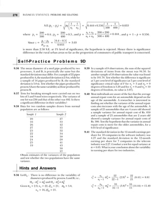
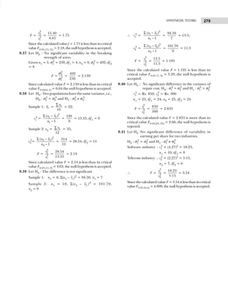
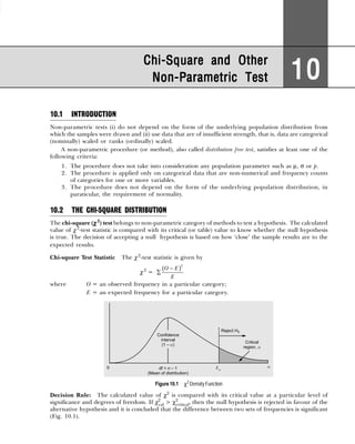
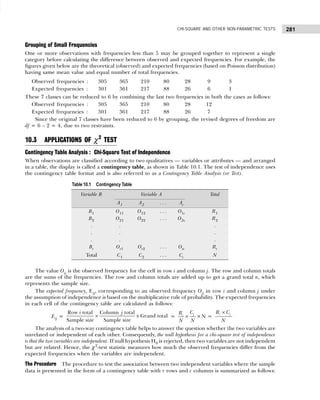
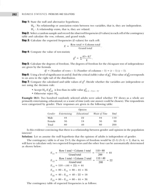
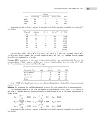
![BUSINESS STATISTICS: PROBLEMS AND SOLUTIONS
284
The critical value of χ2
= 13.30 at α = 0.01 and df = 4. Since calculated value of
χ2
= 9.836 is less than its critical value, the null hypothesis H0 is accepted. Hence we conclude that stress
on the job is independent of commuting time.
Example 10.3: A certain drug is claimed to be effective in curing cold. In an experiment on 500 persons
with cold, half of them were given the drug and half of them were given sugar pills. The patients’
reactions to the treatment are recorded in the following table:
On the basis of the data, can it be concluded that there is a significant difference in the effect of the
drug and sugar pills? [Lucknow Univ., MBA, 1998; Delhi Univ., MBA, 1999, 2002]
Solution: Let us assume the null hypothesis that there is no significant difference in the effect of the drug
and sugar pills.
The contingency table is of size 2 × 3, the degrees of freedom would be (2 – 1) (3 – 1) = 2, that is, we
would have to calculate only two expected frequencies and others can be automatically determined as
shown below:
E11 =
250 280
500
×
= 140; E12 =
250 70
500
×
= 35
The contingency table of expected frequencies is as follows:
Arranging the observed and expected frequencies in the following table to calculate the value of
χ2
-test statistic.
Observed Expected O – E (O – E)2
(O – E)2
/E
(O) (E)
9 12.14 –3.14 9.85 0.811
5 5.24 –0.24 0.05 0.009
18 14.62 3.38 11.42 0.781
17 20.10 –3.10 9.61 0.478
8 8.68 –0.68 0.45 0.052
28 24.22 3.78 14.28 0.589
18 11.75 6.25 39.06 3.324
6 5.08 0.92 0.84 0.165
7 14.17 –7.17 51.40 3.627
9.836
Consequence
Treatment Helped Reaction No Effect Total
Drug 150 30 70 250
Sugar pills 130 40 80 250
Total 280 70 150 500
Consequence
Treatment Helped Harmed No Effect Total
Drug 140 35 75 250
Sugar pills 140 35 75 250
Total 280 70 150 500](https://image.slidesharecdn.com/businessstatisticsproblemsandsolutions-230910073954-6d42a210/85/Business-Statistics_-Problems-and-Solutions-pdf-298-320.jpg)
![285
CHI-SQUARE AND OTHER NON-PARAMETRIC TESTS
The critical value of χ2
= 5.99 at α = 0.05 and df = 2. Since the calculated value of χ2
= 3.522 is less
than its critical value, the null hypothesis is accepted. Hence we conclude that there is no significant
difference in the effect of the drug and sugar pills.
S e l f-P r a c t i c e P r o b l e m s 10A
10.1 In an anti-malaria campaign in a certain area, quinine
was administered to 812 persons out of a total
population of 3248. The number of fever cases
reported is shown below:
Treatment Fever No Fever Total
Quinine 20 792 812
No quinine 220 2216 2436
Total 240 3008 3248
Discuss the usefulness of quinine in checking
malaria. [MD Univ., M.Com., 1998]
10.2 Based on information from 1000 randomly selected
fields about the tenancy status of the cultivation of
these fields and use of fertilizers, collected in an agro-
economic survey, the following classifications were
noted:
Owned Rented Total
Using fertilizers 416 184 600
Not using fertilizers 064 336 400
Total 480 520 1000
Would you conclude that owner cultivators are
more inclined towards the use of fertilizers at α = 0.05
level of significance? Carry out the chi-square test as
per testing procedures.[Osmania Univ., M.Com., 1997]
10.3 In an experiment on immunization of cattle from
tuberculosis, the following results were obtained:
Affected Not Affected
Inoculated 12 26
Not inoculated 16 6
Calculate the χ2
and discuss the effect of vaccine in
controlling susceptibility to tuberculosis.
[Rajasthan Univ., M.Com., 1996]
10.4 From the data given below about the treatment of
250 patients suffering from a disease, state whether
the new treatment is superior to the conventional
treatment.
Treatment No. of Patients
Favourable Not Favourable Total
New 140 30 170
Conventional 60 20 080
Total 200 50 250
[MD Univ., M.Com., 1998]
10.5 1000 students at college level are graded according to
their IQ and their economic conditions. Use chi-square
test to find out whether there is any association between
economic conditions and the level of IQ.
Economic IQ Level
Conditions High Medium Low Total
Rich 160 300 140 600
Poor 140 100 160 400
Total 300 400 300 1000
[Madurai Univ., M.Com., 1996]
10.6 200 digits are chosen at random from a set of tables.
The frequencies of the digits are as follows:
Digit : 0 1 2 3 4 5 6 7 8 9
Frequency: 18 19 23 21 16 25 22 20 21 15
Observed Expected (O – E) (O – E)2
(O – E)2
/E
(O) (E)
150 140 10 100 0.714
130 140 –10 100 0.714
30 35 –5 25 0.714
40 35 5 25 0.714
70 75 –5 25 0.333
80 75 5 25 0.333
3.522](https://image.slidesharecdn.com/businessstatisticsproblemsandsolutions-230910073954-6d42a210/85/Business-Statistics_-Problems-and-Solutions-pdf-299-320.jpg)
![BUSINESS STATISTICS: PROBLEMS AND SOLUTIONS
286
Use the χ2
-test to assess the correctness of the
hypothesis that the digits were distributed in equal
numbers in the tables from which they were chosen.
[HP Univ., M.Com., 2000]
10.7 In an experiment on pea-breeding, Mendel obtained
the following frequencies of seeds: 315 round and
yellow, 101 wrinkled and yellow, 108 round and green,
32 winkled and green. According to his theory of
heredity the numbers should be in proportion 9 : 3 : 3
: 1. Is there any evidence to doubt the theory at
α = 0.05 level of significance?
[Delhi Univ., M.Com., 1996]
10.8 Two researchers adopted different sampling
techniques while investigating the same group of
students to find the number of students falling in
different intelligence levels. The results are as follows:
Researcher Below Average Above Genius Total
Average Average
X 086 060 44 10 200
Y 040 033 25 02 100
Total 126 093 69 12 300
Would you say that the sampling techniques
adopted by the two researchers are significantly
different? [Delhi Univ., MBA, 1998]
10.9 From the following data, find out whether there is any
relationship between sex and preference of colour:
Colour Males Females Total
Red 10 40 50
White 70 30 100
Green 30 20 50
Total 110 90 200
[HP Univ., MBA, 1998; Madurai Univ., M.Com., 1999]
10.10 A manufacturer of TV sets was trying to find out what
variables influenced the purchase of a TV set. Level of
income was suggested as a possible variable
influencing the purchase of TV sets. A sample of 500
households was selected and the information obtained
is classified as shown below:
Income Group Have Do not Have
TV Set TV Set
Low income group 0 250
Middle income group 50 100
High income group 80 20
Is there evidence from the above data of a relation
ownership of TV sets and level of income?
[Delhi Univ., MBA, 2000]
10.11 A marketing agency gives the following information
about the age groups of the sample informants and
their liking for a particular model of scooter which a
company plans to introduce:
Choice Age Group of Informants
Below 20 20–39 40–59 Total
Liked 125 420 060 0605
Disliked 075 220 100 0395
Total 200 640 160 1000
On the basis of above data, can it be concluded that
the model appeal is independent of the age group of
the informants? [HP Univ., MBA, 1998]
Hints and Answers
10.1 Let H0 : Quinine is not effective in checking malaria.
χ2
cal = 38.393 is more than its critical value χ2
critical =
3.84 at α = 0.05 and df = 1, the null hypothesis is
rejected.
10.2 Let H0 : Ownership of fields and the use of fertilizers
are independent attributes.
χ2
cal = 273.504 is more than its critical value χ2
critical =
3.84 at α = 0.05 and df = 1, the null hypothesis is
rejected.
10.3 Let H0 : Vaccine is not effective in controlling
susceptibility to tuberculosis.
χ2
cal =7.796ismorethanitscriticalvalueχ2
critical =3.84
at α = 0.05 and df = 1, the null hypothesis is rejected.
10.4 Let H0 : No significant difference between the new
and conventional treatment.
χ2
cal = 1.839 is less than its critical value χ2
critical = 3.84
at α = 0.05 and df = 1, the null hypothesis is accepted.
10.5 Let H0 : No association between economic conditions
and the level of IQ.
χ2
cal = 65.277 is more than its critical value χ2
critical =
5.99 at α = 0.05 and df = 2, the null hypothesis is
rejected.](https://image.slidesharecdn.com/businessstatisticsproblemsandsolutions-230910073954-6d42a210/85/Business-Statistics_-Problems-and-Solutions-pdf-300-320.jpg)
![287
CHI-SQUARE AND OTHER NON-PARAMETRIC TESTS
10.6 Let H0 : Digits were distributed in equal numbers.
On the basis of H0, E = 200/10 = 20 as the frequency
of occurrence for 0, 1, 2, . . . digits.
χ2
cal = 4.3 is less than its critical value χ2
= 16.22 at α =
0.05anddf =10–1=9,thenullhypothesisisaccepted.
10.7 Let H0 : No significant difference in the observed and
expected frequencies.
Calculations of expected values are as follows:
E1 =
556 9
16
×
= 312.75, E2 =
556 3
16
×
= 104.25,
E3 = 104.25 and E4 = 34.75, respectively.
Category O E (O – E)2
(O – E)2
/E
Round and yellow 315 312.75 5.062 0.016
Wrinkledandyellow 101 104.25 10.562 0.101
Roundandgreen 108 104.25 14.062 0.135
Wrinkledandgreen 032 134.75 07.562 0.218
0.470
Since χ2
cal = 0.470 is less than its critical value
χ2
= 7.82 at α = 0.05 and df = 4 – 1 = 3, the null
hypothesis is accepted.
10.8 Let H0 : Sampling techniques adopted by two
researchers are not significantly different.
χ2
cal = 2.098 is less than its critical value χ2
critical = 7.82
at α = 0.05 and df = 3, the null hypothesis is accepted.
10.9 Let H0 : No relationship between gender and
preference of colour.
χ2
cal = 34.35 is more than its critical value χ2
critical =
5.99 at α = 0.05 and df = 2, the null hypothesis is
rejected.
10.10 Let H0 : The ownership of TV sets is independent of
the level of income.
χ2
cal = 243.59 is more than its critical value χ2
critical =
7.82 at α = 0.05 and df = 2, the null hypothesis is
rejected.
10.11 Let H0 : The model appeal is independent of the age
group of the informants.
χ2
cal = 42.788 is more than its critical value χ2
critical =
5.99 at α = 0.05 and df = 2, the null hypothesis is
rejected.
10.4 CHI-SQUARE TEST FOR GOODNESS-OF-FIT
The χ2
test for goodness-of-fit is a statistical test of how well given data support an assumption about the distribution
of a population or random variable of interest. The test determines how well an assumed distribution fits the given
data. The observed frequencies or values come from the sample and the expected frequencies or values
come from the theoretical hypothesized probability distribution.
The Procedure
Step 1: State the null and alternative hypotheses.
H0 : No difference between the observed and expected sets of frequencies.
H1 : There is a difference.
Step 2: Select a random sample and record the observed frequencies (O values) for each category.
Step 3: Calculate expected frequencies (E values) in each category by multiplying the category probability
by the sample size.
Step 4: Compute the value of test statistic
χ2
=
2
(O E)
E
−
∑
Step 5: Using a level of significance α and df = n – 1 provided that the number of expected frequencies
are 5 or more for all categories, find the critical (table) value of χ2
.
Step 6: Compare the calculated and table value of χ2
, and use the following decision rule:
• Accept H0 if χ2
cal is less than its critical value χ2
α, n – 1
• Otherwise reject H0
Example 10.4: A Personnel Manager is interested in trying to determine whether absenteeism is greater
on one day of the week than on another. His records for the past year show the following sample distribution:
Day of the week : Monday Tuesday Wednesday Thursday Friday
No. of absentees : 66 56 54 48 75
Test whether the absence is uniformly distributed over the week. [Madras Univ., M.Com., 1996]](https://image.slidesharecdn.com/businessstatisticsproblemsandsolutions-230910073954-6d42a210/85/Business-Statistics_-Problems-and-Solutions-pdf-301-320.jpg)
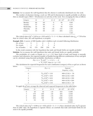
![289
CHI-SQUARE AND OTHER NON-PARAMETRIC TESTS
Mistakes (x) Number of fx
Pages ( f )
0 616 0
1 70 70
2 10 20
3 2 6
4 1 4
5 1 5
n = 700 105
Example 10.6: The figures given below are (a) the theoretical frequencies of a distribution and (b) the
frequencies of the normal distribution having the same mean, standard deviation, and the total frequency
as in (a):
(a) 1 5 20 28 42 22 15 5 2
(b) 1 6 18 25 40 25 18 6 1
Do you think that the normal distribution provides a good fit to the data?
Solution: Let us assume the null hypothesis that there is no difference between observed frequencies and
expected frequencies obtained by normal distribution.
Since the observed and expected frequencies are less than 10 in the beginning and end of the series,
we shall group these classes together as follows:
The revised degrees of freedom are df = 9 – 1 – 4 = 4. The critical value χ2
critical = 9.49 at α = 0.05
and df = 4. Since the calculated value of χ2
= 1.685 is less than its critical value, the null hypothesis is
accepted. Hence, we conclude that the normal distribution provides a good fit to the data.
Example 10.7: A book has 700 pages. The number of pages with various numbers of misprints is recorded
below:
No. of misprints : 0 1 2 3 4 5
No. of pages with misprints : 616 70 10 2 1 1
Can a Poisson distribution be fitted to this data? [Delhi Univ., M.Com., 1999]
Solution: Let us assume the null hypothesis that the data is fitted with Poisson distribution.
The number of pages in the book are 700, whereas the maximum possible number of misprints are
only 5. Thus we may apply Poisson probability distribution to calculate the expected number of misprints
in each page of the book as follows:
λ or m =
fx
n
Σ
=
105
700
= 0.15.
O E O – E (O – E)2
(O – E)2
/E
1
5
= 6
1
6
= 7 –1 1 0.143
20 18 2 4 0.222
28 25 3 9 0.360
42 40 2 4 0.100
22 25 –3 9 0.360
15 18 –3 9 0.500
5
2
= 7
6
1
= 7 0 0 0.000
1.685](https://image.slidesharecdn.com/businessstatisticsproblemsandsolutions-230910073954-6d42a210/85/Business-Statistics_-Problems-and-Solutions-pdf-303-320.jpg)
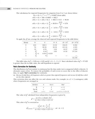
![291
CHI-SQUARE AND OTHER NON-PARAMETRIC TESTS
and
2
corrected
χ =
2
1
2
( ) ( ) ( ) ( )
n bc ad n
a b c d a c b d
− −
+ + + +
; ad – bc < 0.
(b) An alternative formula for calculating the χ2
test statistic is as follows:
χ2
=
{ }2
|O E| 0.5
E
− −
∑ .
Example 10.8: Of the 1000 workers in a factory exposed to an epidemic, 700 in all were attacked, 400
had been inoculated, and of these 200 were attacked. On the basis of this information, can it be believed
that inoculation and attack are independent? [HP Univ., MBA, 1998]
Solution: Let us assume the null hypothesis that there is no association between inoculation and attack,
that is, inoculation and attack are independent.
The given information can be arranged in a 2 × 2 contingency table as follows:
Using the result of Section 11.4.3, we have a = 200, b = 200, c = 500, d = 100, and n = 1000. Thus,
χ2
=
2
( ) ( )
( ) ( ) ( ) ( )
a b c d ab bc
a b c d a c b d
+ + + −
+ + + +
=
2
1000 (200 100 200 500)
(200 200) (500 100) (200 500) (200 100)
× − ×
+ + + +
=
2
1000 (80,000)
400 600 700 300
×
× × ×
=
×
1000 64
504
= 126.984.
The critical value of χ2
= 3.84 at α = 0.05 and df = (2 – 1) (2 – 1) = 1. Since calculated value χ2
cal =
126.984 is more than its critical value, the null hypothesis rejected. Hence, we conclude that inoculation
and attack are not independent.
Example 10.9: The following information was obtained in a sample of 40 small general shops:
Can it be said that there are relatively more women owners of small general shops in rural than in
urban areas?
Solution: Let us assume the null hypothesis that there are an equal number of men and women owners
of small shops in both rural and urban areas.
Since one of the frequencies is small, we apply Yate’s correction formula to calculate χ 2
as follows:
Here a = 17, b = 18, c = 3, d = 12, and n = 50
2
corrected
χ =
2
1
2
( ) ( ) ( ) ( )
n ad bc n
a b c d a c b d
− −
+ + + +
=
2
1
50 17 12 18 3 50
2
35 15 20 30
× − × − ×
× × ×
=
2
50 (204 54 25)
35 15 20 30
− −
× × ×
=
× ×
× × ×
50 125 125
35 15 20 30
= 2.480.
Attributes Attacked Not Attacked Total
Inoculated 200 200 400
Not inoculated 500 100 600
Total 700 300 1000
Shops in
Owner Urban Areas Rural Areas Total
Men 17 18 35
Women 03 12 15
Total 20 30 50](https://image.slidesharecdn.com/businessstatisticsproblemsandsolutions-230910073954-6d42a210/85/Business-Statistics_-Problems-and-Solutions-pdf-305-320.jpg)
![BUSINESS STATISTICS: PROBLEMS AND SOLUTIONS
292
The critical value of χ 2
= 3.841 at α = 0.05 and df = (2 – 1) (2 – 1) = 1. Since calculated value χ 2
=
2.480 is less than its critical value χ 2
= 3.841, the null hypothesis is accepted. Hence we conclude that
shops owned by men and women in both areas are equal in number.
S e l f-P r a c t i c e P r o b l e m s 10B
10.12 A sample analysis of examination results of 500
students was made. It was found that 220 students
had failed, 170 had secured a third class, 90 were placed
in second class, and 20 got a first class. Are these
figures commensurate with the general examination
result which is in the ratio of 4 : 3 : 2 : 1 for the various
categories respectively. [Delhi Univ., M.Com., 1999]
10.13 A set of 5 coins are tossed 3200 times, and the number
of heads appearing each time is noted. The results are
given below:
No. of heads : 0 1 2 3 4 5
Frequency : 80 570 1100 900 50 50
Test the hypothesis that the coins are unbiased.
[Annamalai Univ., M.Com., 1998;
MD Univ., M.Com., 1998]
10.14 The demand for a particular spare part in a factory
was found to vary from day to day. In a sample study
the following information was obtained:
Day : Mon. Tues. Wed. Thurs. Fri. Sat.
No. of parts
demanded : 1124 1125 1110 1120 1126 1115
Test the hypothesis that the number of parts demanded
does not depend on the day of the week.
[Delhi Univ., MBA, 2002]
10.15 The number of scooter accidents per week in a certain
town were as follows:
12 8 20 2 14 10 15 6 9 4
Are these frequencies in agreement with the belief
that accident conditions were the same during this 10-
week period?
[Delhi Univ., MBA, 2000; HP Univ., M.A. (Eco.), 1997]
10.16 The divisional manager of a chain of retail stores
believes the average number of customers entering
each of the five stores in his division weekly is the
same. In a given week, a manager reports the following
number of customers in his stores: 3000, 2960, 3100,
2780, 3160. Test the divisional manager’s belief at the
10 per cent level of significance
[Delhi Univ., MBA, 2001]
10.17 Figures given below are (a) the theoretical frequencies
of a distribution and (b) the frequencies of the Poisson
distribution having the same mean and total frequency
as in (a).
(a) 305 365 210 80 28 9 3
(b) 301 361 217 88 26 6 1
Apply the χ2
test for goodness-of-fit.
Hints and Answers
10.12 LetH0 :Nodifferenceinobservedandexpectedresults.
Category O E (O – E)2
(O – E)2
/E
Failed 220 500(4/10) = 200 400 2.000
3rd class 170 500(3/10) = 150 400 2.667
2nd class 90 500(2/10) = 100 100 1.000
1st class 20 500(1/10) = 50 900 18.000
23.667
Since χ2
cal = 23.667 is more than its critical value
χ2
= 7.81 for df = 4 – 1 = 3 and α = 0.05, the null
hypothesis is rejected.
10.13 Let H0 : Coins are unbiased, that is, p = q = 1/2.
Apply binomial probability distribution to get the
expected number of heads as follows:
Expected number of heads = n n
Cr pr
qn – r
= 3200 5
C0
5
1 1
2 2
r r
−
= 3200 5
C0
5
1
2
O E (O – E)2
(O – E)2
/E
80 100 400 4.00
570 500 4900 9.80
1100 1000 10,000 10.00
900 1000 10,000 10.00
500 500 0 0.00
50 100 2500 25.00
58.80](https://image.slidesharecdn.com/businessstatisticsproblemsandsolutions-230910073954-6d42a210/85/Business-Statistics_-Problems-and-Solutions-pdf-306-320.jpg)
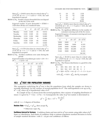
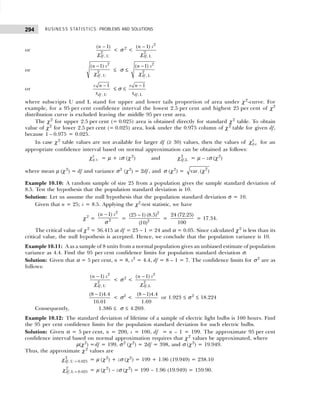
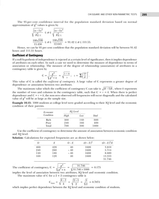
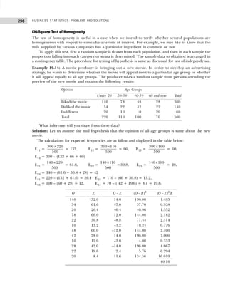
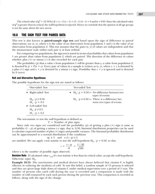
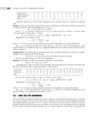
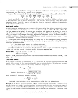
![BUSINESS STATISTICS: PROBLEMS AND SOLUTIONS
300
Test whether the distribution of these movements is random or not at α = 0.05 level of significance.
Solution: Let us state the null and alternative hypotheses as follows:
H0 : Movement is random and H1: Movement is not random.
There are r = 8 runs (plus signs) with n1 = 8 plus (number of increases) and n2 = 6 minus (number
of decreases) so that n = n1 + n2 = 14. The critical vlaue of r = 8 for n1 = 8 and n2 = 6 implies that H0
is rejected when r ≤ 3 and r ≥ 12 at α = 0.05 level of significance. Since 3 ≤ r ≤ 12, H0 cannot be rejected.
Example 10.18: Some items produced by a machine are defective. If the machine follows some pattern
where defective items are not randomly produced throughout the process the machine needs to be
adjusted. A quality control engineer wants to determine whether the sequence of defective (D) versus
good (G) items is random. The data are
GGGGG, DDD, GGGGGG, DDD, GGGGGGGGGG, DDDD,
GGGGGGGGGGG, DDD, GGGGGGGGGGG, DDDD
Test whether the distribution of defective and good items is random or not at α = 0.05 level of
significance.
Solution: Let us state the null and alternative hypotheses as follows:
H0 : Sequence is random and H1 : Sequence is not random.
There are r = 10 runs with n1 = 43 (number of G) and n2 = 17 (number of D), so that n = n1 + n2 =
60. Since sample size is large, we compute mean and standard deviation as follows:
Mean, µR =
1 2
1 2
2
1
n n
n n
+
+
=
2 43 17
1
43 17
× ×
+
+
= 24.8
Standard deviation, σR = 1 2 1 2 1 2
2
1 2 1 2
2 (2 )
( ) ( 1)
n n n n n n
n n n n
− −
+ + −
= 2
2(43)(17)[2(43)(17) 43 17]
(43 17) (43 17 1)
− −
+ + −
=
1462 1402
3600 59
×
×
=
20,49,724
2,12,400
= 3.106
The computed value of z-test statistic is
z = R
R
R − µ
σ
=
10 24.8
3.106
−
= – 7.871.
The critical value of zα = 2.58 for two-tailed test at α=0.05 level of significance. Since zα < zcal, H0 is
rejected. Hence, we conclude that the sequence of defective versus good item is not random.
10.8 MANN–WHITNEY U-TEST
To apply the U-test, also called the Wilcoxon rank sum test or simply the Rank Sum Test, values from two
samples are combined into one group and are arranged in ascending order. The pooled values are then
ranked from 1 to n with smallest value being assigned a rank 1. Such a test produces good results when
data are on ordinal scale of measurement. The sum of ranks of values from sample 1 is denoted as R1.
Similarly, the sum of the ranks of values from sample 2 is denoted as R2. If both n1 and n2 < 30, samples
are considered small. If either n1 or n2 is greater than 10, the samples are considered large.
Small Sample U-Test
1. Combine the two random samples of size n1 and n2 and rank values from smallest to largest. If several
values are tied, then assign each the average of the ranks that would otherwise have been assigned.
If the two sample sizes are unequal, then suppose n1 represent smaller-sized sample and n2 represent
the larger-sized sample. The rank sum test statistic U1 is the sum of the ranks assigned to the n1
observations in the smaller sample. However, for equal-sized samples, either group may be selected
for determining U1.](https://image.slidesharecdn.com/businessstatisticsproblemsandsolutions-230910073954-6d42a210/85/Business-Statistics_-Problems-and-Solutions-pdf-314-320.jpg)
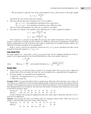
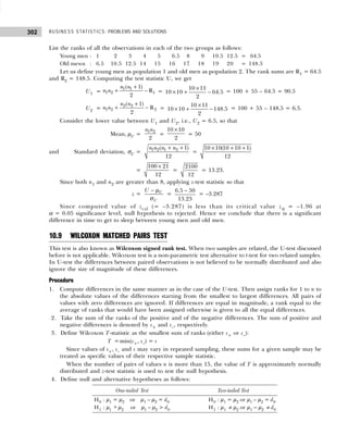
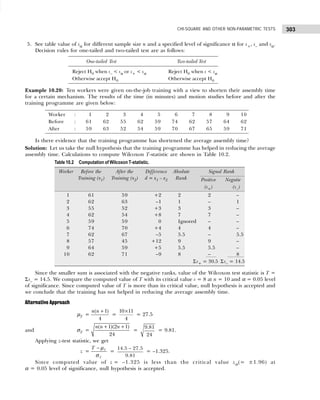
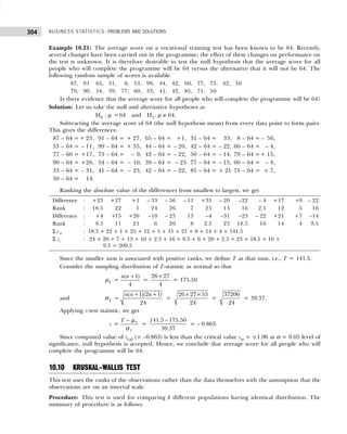
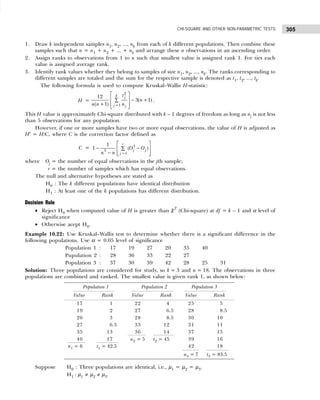
![BUSINESS STATISTICS: PROBLEMS AND SOLUTIONS
306
Kruskal–Wallis test statistic is
H′ =
H
C
,
where H =
3
2
1
12
( / ) 3( 1)
( 1)
j j
j
t n n
n n =
− +
∑
+
=
2 2 2
12 (42.5) (45) (83.5)
3 19
18 19 6 5 7
+ + − ×
×
= 0.035[(301.4 + 405 + 996.03)] – 57 = 2.572
and C =
2
3
3
1
1
1 ( )
j j
j
O O
n n =
− −
∑
−
= 3 2
3
1
1 [{(2) 2} {(2) 2}]
(18) 18
− − + −
−
=
12
1
5814
− = 1 – 0.002 = 0.998.
Thus, H′ =
2.572
0.998
= 2.577.
Since computed value of H′ (= 2.577) is less than table value of χ2
(= 5.99) at df =
k – 1 = 2 and α = 0.05, the null hypothesis is accepted and it is concluded that three populations are
identical.
10.11 MISCELLANEOUS SOLVED EXAMPLES
Example 10.23: Based on information on 1000 randomly selected fields about the tenancy status of the
cultivation of these fields and use of fertilizers, collected in an agro-economic survey, the following
classification was noted:
Owned Rented Total
Using fertilizers 416 184 600
Not using fertilizers 64 336 400
Total 480 520 1000
Would you conclude that owner cultivators are more towards the use of fertilizers at 5% level? Carry out
chi-square test as per testing procedure. [Osmania Univ., M.Com., 2005]
Solution: Let us take the hypothesis that ownerships of fields and the use of fertilizers are independent
attributes.
Using the following formula to calculate expected frequencies corresponding to the given (observed)
frequencies:
Eij =
Row total ×columing total
Ground total
i j
.
The table of corresponding expected frequencies shall be
E11 = 288 E12 = 312 E13 = 600
E21 = 192 E22 = 208 E23 = 400
The contingency table of expected frequencies is as follows:
Observed (O) Expected (E) (O – E)2
χ2
= (O – E)2
/E
416 288 16,384 56.889
64 192 16,384 85.333
184 312 16,384 52.513
336 208 16,384 78.769
273.534](https://image.slidesharecdn.com/businessstatisticsproblemsandsolutions-230910073954-6d42a210/85/Business-Statistics_-Problems-and-Solutions-pdf-320-320.jpg)
![307
CHI-SQUARE AND OTHER NON-PARAMETRIC TESTS
The calculated value of χ2
= 273.534 at α = 0.05 and df = (n – 1)(r – 1) = (2 – 1)(2 – 1) = 1 is much
more than the table value χ2
= 3.84. The null hypothesis H0 is rejected. Hence it can be concluded that
owners cultivators are more inclined towards the use of fertilizers.
Example 10.24: In an experiment on immunization of cattle from tuberculosis, the following results
were obtained:
Affected Not Affected Total
Inoculated 12 26 38
Not inoculated 16 6 22
28 32
Calculate χ2
and discuss the effect of vaccine in controlling susceptibility to tuberculosis (5% value of
χ2
for one degree of freedom = 3.84) [Univ. of Kashmir, M.Com., 2005; Madras Univ., B.Com., 2006]
Solution: Let us take the hypothesis that the vaccine is not effective in controlling susceptibility to
tuberculosis.
Since one of the observed frequencies is less than 10, we will use Yates’ correction formula to calculate
χ2
as follows:
Here a = 12, b = 26, c = 16, d = 6, and n = 50.
χ2
corrected =
− −
+ + + +
2
( 1/2 )
( )( )( ) ( )
n ad bc n
a b c d a c b d
=
× − × − ×
+ + + +
2
50(12 6 26 16 1/ 2 50)
(12 26)(16 6)(12 16)(26 6)
=
−
× × ×
2
50( 369)
38 32 28 32
=
6808050
749056
= 9.08.
Since the calculated value of χ2
= 9.088 at α = 0.05 and df = (c – 1)(r – 1) = (2 – 1)(2 – 1) = 1 is greater
than the table value χ2
= 3.84, the null hypothesis H0 is rejected. Hence, we conclude that the vaccine is
effective in controlling susceptibility to tuberculosis.
Example 10.25: 200 digits are chosen at random from a set of tables. The frequencies of the digits are as
follows:
Digit : 0 1 2 3 4 5 6 7 8 9
Frequency : 18 19 23 21 16 25 22 20 21 15
Use χ2
test to assess the correctness of the hypothesis that the digits were distributed in equal numbers in
the table from which they were chosen. [HP Univ., M.Com., 2000; Chennai Univ., B.Com., 2005]
Solution: Let us take the hypothesis that the digits were distributed in equal numbers. Since total of
frequencies is 200, and the selection of each digit is equally probable, we should expect 200/10 = 20 as
the frequency of 1, 1, 2, ...., digits. Arranging the data as follows:
Digit O E (O – E)2
χ2
= (O – E)2
/E
0 18 20 4 0.20
1 19 20 1 0.05
2 23 20 9 0.45
3 21 20 1 0.80
4 16 20 16 0.80
5 25 20 25 1.25
6 22 20 4 0.20
7 20 20 0 0.00
8 21 20 1 0.05
9 15 20 25 1.25
200 4.3](https://image.slidesharecdn.com/businessstatisticsproblemsandsolutions-230910073954-6d42a210/85/Business-Statistics_-Problems-and-Solutions-pdf-321-320.jpg)
![BUSINESS STATISTICS: PROBLEMS AND SOLUTIONS
308
Since the calculated of χ2
= 4.3 is less than the table value χ2
= 16.22 at α = 0.05 and df = 10 – 1 = 9,
the hypothesis that the digits were distributed in equal numbers is accepted.
Example 10.26: In an experiment on pea-breeding, Mendel obtained the following frequencies of speed:
315 round and yellow, 101 wrinkled and yellow, 108 round and green, 32 wrinked and green. According
to his theory of heredity the numbers should be in proportion 9 : 3 : 3 : 1. Is there any evidence to doubt
the theory at 5% level of significance? [Delhi Univ., M.Com., 2004]
Solution: Let us take the hypothesis that there is no significant difference in the observed and expected
frequencies.
According to the theory the expected frequencies should be
E1 =
×
556 9
16
= 312.75; E2 =
×
556 3
16
= 104.25; E3 = 104.25; and E4 = 34.75; respectively.
The contingency table of expected frequencies is as follows:
Category O E (O – E)2
χ2
= (O – E)2
/E
Round & Yellow 315 312.75 5.0625 0.016
Wrinkled & Yellow 101 104.25 10.5625 0.101
Round & Green 108 104.25 14.0625 0.135
Wrinkled & green 32 34.75 7.5625 0.218
0.47
v = n – 1 = 4 – 1 = 3
v = 3, χ2
0.05 = 7.82.
The calculated value of χ2
= 0.47 is less than the table value χ2
= 7.82 at α = 0.05 and df = n – 1 =
4 – 1 = 3. The hypothesis is accepted. Hence there is no evidence to doubt the theory.
Example 10.27: A sample analysis of examination results of 500 students was made. It was found that 220
students had failed, 170 had secured a third class, 90 were placed in second class, and 20 got a first class.
Are these figures commensurate with the general examination result which is the ratio of 4 : 3 : 2 : 1 for
the various categories respectively (the table value of χ2
for 3 d.f. at 5% levels of significance is 7.81)?
[Delhi Univ., M.Com., 2003]
Solution: Let us take the null hypothesis that the observed results are commensurate with the general
examination result which is the ratio of 4 : 3 : 2 : 1.
The expected number of students who have failed, obtained a third class, second class, and first class,
respectively, are
E1 =
×
500 4
4
= 200; E2 =
×
500 3
10
= 150; E3 =
×
500 1
10
= 100; and E4 =
×
500 1
10
= 50.
The contingency table of expected and observed frequencies is as follows:
Category O E (O – E)2
χ2
= (O – E)2
/E
Failed 220 200 400 2.000
3rd class 170 150 400 2.667
2nd class 90 100 100 1.000
1st class 20 50 900 18.000
23.667
Since the calculated value of χ2
= 23.667 is greater than the table value χ2
= 7.81 at α = 0.05 and
df = n – 1 = 4 – 1 = 3, the hypothesis is rejected.](https://image.slidesharecdn.com/businessstatisticsproblemsandsolutions-230910073954-6d42a210/85/Business-Statistics_-Problems-and-Solutions-pdf-322-320.jpg)
![309
CHI-SQUARE AND OTHER NON-PARAMETRIC TESTS
Example 10.28: A movie producer is bringing out a new movie. In order to map out his advertising
campaigns, he wants to determine whether the movie will appeal most of particular age group or whether
it will appeal equally to all age groups. The producer takes a random sample from persons attending
preview of the new movie and obtains the following results:
Age Group
Choice
Under 20 20–39 40–59 60 and over Total
Liked the movie 146 78 48 28 300
Disliked the movie 54 22 42 22 140
Indifferent 20 10 10 20 60
Total 220 110 100 70 500
What inference will you draw from this data? [Kashmir Univ., M.Com., 2007]
Solution: Let us take the null hypothesis that the movie appeals equally to all age groups.
Using the following formula to calculate expected frequencies corresponding to observed frequencies
as follows:
E11 =
300
220 =132;
200
× E12 =
300
110= 66;
500
× E13 =
300
100 =60
500
× ;
E21 =
140
220 = 61.6
500
× ; E22 =
140
110 = 30.8
500
× ; E23 =
140
100 = 28
500
× .
The contingency table so obtained is given below:
O E (O – E)2
χ2
= (O – E)2
/E
146 132.0 196.0 1.485
54 61.6 57.76 0.938
20 26.4 40.96 1.552
78 66.0 144.00 2.182
22 30.8 77.44 2.514
10 13.2 10.24 0.776
48 60.0 144.00 2.400
42 28.0 196.00 7.000
10 12.0 4.00 0.333
28 42.0 196.00 4.667
22 19.6 5.76 0.294
20 8.4 134.56 16.019
40.16
The calculated value of χ2
= 40.16 is greater than the table value χ2
= 12.59 at α = 0.05 and
df = (r – 1)(c – 1) = (3 – 1)(4 – 1) = 6. The hypothesis is rejected and hence we conclude that the movie
does not appeal equally to all age groups.
Example 10.29: From the adult male population of seven large cities random samples of married and
unmarried men as given below was taken. Can it be said that there is a significant variation among the
people of different cities in the tendency to marry?
City : A B C D E F G Total
Married : 170 285 165 106 153 125 146 1,150
Unmarried : 40 125 35 37 53 35 33 360
210 410 200 143 208 160 179 1,510
[Punjab Univ., M.Com., 1997; Tamil Nadu Univ., MBA, 2005]](https://image.slidesharecdn.com/businessstatisticsproblemsandsolutions-230910073954-6d42a210/85/Business-Statistics_-Problems-and-Solutions-pdf-323-320.jpg)
![BUSINESS STATISTICS: PROBLEMS AND SOLUTIONS
310
Solution Let us take the hypothesis that there is no significant different in the tendency of men to marry
in different cities.
Expected number of married and unmarried men in different cities are calculated as follows:
E11 =
1150
210 =159.93;
1510
× E12 =
1150
410= 312.25
1510
× ; E13 =
1150
200 =152.32;
1510
×
E14 =
1150
143=108.91
1510
× ; E15 =
1150
208=158.41;
1510
× E16 =
1150
160 =121.85;
1510
×
E17 =
1150
179 =136.33
1510
× , and so on
The contingency table so obtained is given below:
O E (O – E)2
χ2
= (O – E)2
/E
170 159.93 101.405 0.634
285 312.25 742.562 2.378
165 152.32 160.782 1.056
106 108.91 8.468 0.078
153 158.41 29.268 0.185
125 121.85 9.922 0.081
146 136.33 93.509 0.686
40 50.07 101.405 2.025
125 97.75 742.562 7.597
35 47.68 1650.752 3.372
37 34.09 8.468 0.248
55 49.59 29.268 0.590
35 38.15 9.922 0.260
33 42.67 93.509 2.191
21.381
The calculated value of χ2
= 21.381 is greater than the table value χ2
= 12.59 at α = 0.05 and
df = (r – 1)(c – 1) = (2 – 1)(7 – 1) = 6. The hypothesis is rejected, and hence we conclude that there is
difference in the tendency of people to marry in different cities.
Example 10.30: A set of 5 coins are tossed 3200 times and the number of heads appearing each time is
noted. The results are given below:
No. of heads : 0 1 2 3 4 5
Frequency : 80 570 1,100 900 500 50
Test the hypothesis that the coins are unbiased.
[Annamalai Univ., M.Com., 1996; Chennai Univ., B.Com., 2005]
Solution: Let us take the null hypothesis that the coins are unbiased. Then the changes of getting heads
in a toss of 5 coins are the successive terms of the binomial expansion
5
1 1
2 2
+
. So the theoretical
frequencies in 3200 tosses are the term in the expansion:
3200
5
1 1
2 2
+
and are as follows :
No. of heads : 0 1 2 3 4 5
Frequencies : 100 500 1,000 1,000 500 100](https://image.slidesharecdn.com/businessstatisticsproblemsandsolutions-230910073954-6d42a210/85/Business-Statistics_-Problems-and-Solutions-pdf-324-320.jpg)
![311
CHI-SQUARE AND OTHER NON-PARAMETRIC TESTS
The contingency table so obtained is as follows:
O E (O – E)2
χ2
= (O – E)2
/E
80 100 400 4.00
570 500 4,900 9.80
1,100 1,000 10,000 10.00
900 1,000 10,000 10.00
500 500 0 0.00
50 100 2,500 25.00
58.80
The calculated value of χ2
= 58.80 is greater than the table value χ2
= 11.07 at α = 0.05 and df = n
– 1 = 6 – 1 = 5. The hypothesis is rejected, and hence we conclude that the coins are biased.
Example 10.31: The following results were obtained when two sets of items were subjected to two different
treatments X and By, to enhance their tensile strength.
Treatment X was applied on 400 items and 80 were found to have gained in stength.
Treatment By was applied in 400 items and 20 were found to have gained in strength.
Is treatment Y supplier to treatment X? [Madras Univ., 2001]
Solution: Let us take the null hypothesis that there is no difference in the two types of treatments
X and Y.
The given results can be tabulated as follows:
Treatment Gained Not Gained Total
X 80 320 400
Y 20 380 400
Total 100 700 800
The expected frequencies corresponding to the observed frequencies are calculated as follows:
E11 = 50; E12 = 350; E21 = 50; E22 = 350
Arranging the observed and expected frequencies as follows:
O E (O – E)2
χ2
= (O – E)2
/E
80 50 900 18.000
20 50 900 18.000
320 350 900 2.571
380 350 900 2.571
41.142
The calculated value of χ2
= 41.42 is higher than the table value χ2
= 3.84 at α = 0.05 and
df = (r – 1)(c – 1) = (2 – 1)(2 – 1) = 1. The hypothesis is rejected, and hence we conclude that there is
difference in treatments X and Y.
Example 10.32: Given below is the contingency table for production in three shifts and the number of
defective goods turnout. Find the value of C = 2 2
N +
χ χ . Is it possible that the number of defective
goods depends on the shift run by the factory?](https://image.slidesharecdn.com/businessstatisticsproblemsandsolutions-230910073954-6d42a210/85/Business-Statistics_-Problems-and-Solutions-pdf-325-320.jpg)
![BUSINESS STATISTICS: PROBLEMS AND SOLUTIONS
312
No. of Defective Goods in 3 Weeks
Shift 1st week 2nd week 3rd week Total
I 15 5 20 40
II 20 10 20 50
III 25 15 20 60
Total 60 30 60 150
[Sri Venketeswara Univ., M.Com., 2006]
Solution: Let us take the null hypothesis that the number of defective goods does not depend on the shift
run by the factory.
The expected frequencies corresponding to observed frequencies are calculated as follows:
E11 = ×
40
60 =16
150
; E21 = ×
50
60 = 20
150
; E12 = ×
40
30 =8
150
; E22 = ×
50
30 =10
150
.
The expected and observed frequencies arranged are as follws:
O E (O – E)2
χ2
= (O – E)2
/E
15 16 1 0.063
20 20 0 0.000
25 24 1 0.042
5 8 9 1.125
10 10 0 0.000
15 12 9 0.750
20 16 16 1.000
20 20 0 0.000
20 24 16 0.667
3.647
Now the coefficient of contingency C =
2
2
3.647 3.647
= =
12.395
150 3.647
N +
+
χ
χ
= 0.294.
The low value of C = 0.294 indicates the poor level of association between shifts and number of defective
goods.
Since the calculated value of χ2
= 3.647 is less than the table value χ2
= 9.438 at α = 0.05 and
df = (r – 1)(c – 1) = (3 – 1)(3 – 1) = 4, the hypothesis is accepted. Hence, the number of defective goods
does not depend on the shift run by the factory.
Example 10.33: A typing school claims that in a six-week intensive course, it can course, it can train
students to type, on the average, at least 60 words per minute. A random sample of 15 graduates is given
a typing test and the median number of words per minute typed by each of these students is given below.
Test the hypothesis that the median typing speed of graduates is at least 60 words per minute.](https://image.slidesharecdn.com/businessstatisticsproblemsandsolutions-230910073954-6d42a210/85/Business-Statistics_-Problems-and-Solutions-pdf-326-320.jpg)
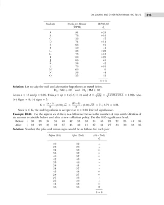
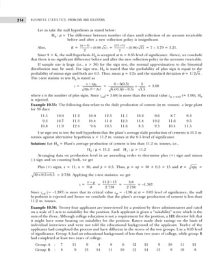
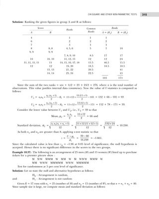
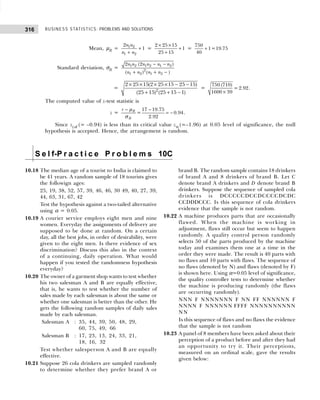
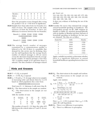
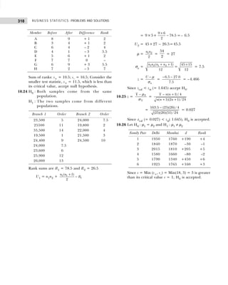
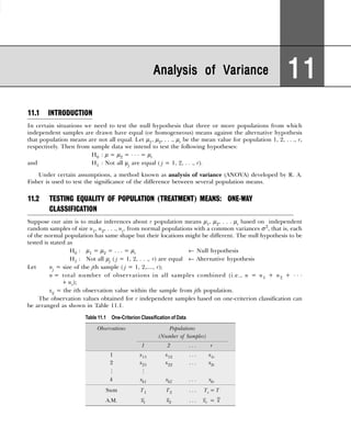
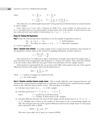
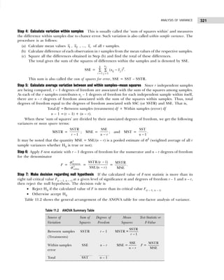
![BUSINESS STATISTICS: PROBLEMS AND SOLUTIONS
322
Short-Cut Method The values of SSTR and SSE can be calculated by applying the following short-cut
methods:
• Calculate the grand total of all observations in samples, T
T = Σ x1 + Σ x2 + . . . + Σ xr
• Calculate the correction factor CF =
2
T
n
; n = n1 + n2 + . . . + nr
• Find the sum of the squares of all observations in samples from each of r samples and subtract CF
from this sum to obtain the total sum of the squares of deviations SST:
SST = (Σx1
2
+ Σx2
2
+ . . . + Σxr
2
) – CF =
2
1 1
j
n
k
ij
i j
x
= =
∑ ∑ – CF
SSTR =
2
( )
Σ j
j
x
n
– CF
and SSE = SST – SSTR.
Example 11.1: To test the significance of variation in the retail prices of a commodity in three principal
cities, Mumbai, Kolkata, and Delhi, four shops were chosen at random in each city and the prices who
lack confidence in their mathematical ability observed in rupees were as follows:
Mumbai : 16 8 12 14
Kolkata : 14 10 10 6
Delhi : 4 10 8 8
Do the data indicate that the price in the three cities are significantly different?
[Jammu Univ., M.Com., 1997]
Solution: Let us take the null hypothesis that there is no significant difference in the prices of a commodity
in the three cities. Calculations for analysis of variance are as under.
There are r=3 treatments (samples) with n1=4, n2=4, n3=4, and n=12.
T = Sum of all the observations in the three samples
= Σx1 + Σx2 + Σx3 = 50 + 40 + 30 = 120
CF = Correction factor =
2
T
n
=
2
(120)
12
= 1200
SST = Total sum of the squares
= (Σx1
2
+ Σx2
2
+ Σx3
2
) – CF = (660 + 432 + 244) – 1200 = 136
SSTR = Sum of squares between the samples
=
2
2 2
2
1 3
1 2 3
( )
( ) ( )
x
x x
n n n
Σ
Σ Σ
+ +
– CF
Sample 1 Sample 2 Sample 3
Mumbai Kolkata Delhi
x1 x1
2
x2 x2
2
x3 x3
2
16 256 14 196 4 16
28 64 10 100 10 100
12 144 10 100 8 64
14 196 6 36 8 64
Σ x1 = 50 Σ x1
2
= 660 Σ x2 = 40 Σ x2
2
= 432 Σ x3 = 30 Σ x3
2
= 244](https://image.slidesharecdn.com/businessstatisticsproblemsandsolutions-230910073954-6d42a210/85/Business-Statistics_-Problems-and-Solutions-pdf-336-320.jpg)
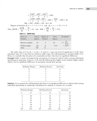
![BUSINESS STATISTICS: PROBLEMS AND SOLUTIONS
324
There are r = 3 treatments (samples) with n1
= n2
= n3
= 6, and n = 18.
T = Sum of all the observations in three samples
= Σ x1
+ Σ x2
+ Σ x3
= 30 + 27 + 36 = 93
CF = Correction factor =
2
T
n
=
2
(93)
18
= 480.50
SST = Total sum of the squares
= (Σx1
2
+ Σx2
2
+ Σx3
2
) – CF = (154 + 123 + 218) – 480.50
= 14.50
SSTR = Sum of squares between the samples
=
2
2 2
2
1 3
1 2 3
( )
( ) ( )
x
x x
n n n
Σ
Σ Σ
+ +
– CF =
2 2 2
(30) (27) (36)
6 6 6
+ +
– 480.50
=
900 729 1296
6 6 6
+ +
– 480.50
= (150 + 121.5 + 216) – 480.50 = 7
SSE = SST – SSTR = 14.50 – 7 = 7.50.
Degrees of freedom: df1
= r – 1=3 – 1=2 and df2
= n – r=18 – 3=15.
Thus, MSTR =
1
SSTR
df
=
7
2
= 3.5 and MSE =
2
SSE
df
=
7.50
15
= 0.5.
The table value of F for df1 = 2, df2 = 15, and α = 0.05 is 3.68. Since calculated value of F = 7 is more
than its table value, the null hypothesis is rejected (Table 11.4). Hence we conclude that there is significant
difference in ethical values among individuals specializing in marketing.
Example 11.3: As head of the department of a consumer’s research organization, you have the responsibility
for testing and comparing lifetimes of four brands of electric bulbs. Suppose you test the life-time of three
electric bulbs of each of the four brands. The data are shown below, each entry representing the lifetime
of an electric bulb, measured in hundreds of hours:
Can we infer that the mean lifetimes of the four brands of electric bulbs are equal?
[Roorkee Univ., MBA, 2000]
Table 11.4 ANOVA Table
Source of Sum of Degrees of Mean Test-Statistic
Variation Squares Freedom Squares
Between samples 7 2 3.5 F =
3.5
0.5
Within samples 7.5 15 0.5 = 7
Total 14.5 17
Brand
A B C D
20 25 24 23
19 23 20 20
21 21 22 20](https://image.slidesharecdn.com/businessstatisticsproblemsandsolutions-230910073954-6d42a210/85/Business-Statistics_-Problems-and-Solutions-pdf-338-320.jpg)
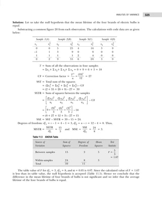
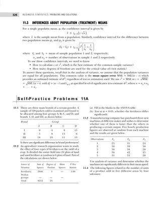
![327
ANALYSIS OF VARIANCE
Area Number of Units
A B C D
1 80 100 95 70
2 82 110 90 75
3 88 105 100 82
4 85 115 105 88
5 75 90 80 65
Is there a significant difference in the efficiency of these
salesmen? [Osmania Univ., MBA, 1998]
11.5 Four machines A, B, C, and D are used to produce a
certain kind of cotton fabric. Samples of size 4 with
each unit as 100 square metres are selected from the
outputs of the machines at random, and the number
of flowers in each 100 square metres is counted, with
the following results:
Machines
A B C D
8 6 14 20
9 8 12 22
11 10 18 25
12 4 9 23
Do you think that there is significant difference in the
performance of the four machines?
[Kumaon Univ., MBA, 1998]
H i n t s a n d A n s w e r s
11.1 Let H0 : There is no significant difference in brand
preference.
Source of Sum of Degrees of Mean Test Statistic
Variation Squares Freedom Square
Between 168.5 12 84.25 F =
84.25
22.83
Samples
= 3.69
Within 205.5 19 22.83
Samples
Total 374.0 11
Since calculated value of F = 3.69 is less than its table
value F = 4.26 at df1 = 2, df2 = 9, and α = 0.05, the
null hypothesis is accepted.
11.2 Given total number of observations, n = 24; Number
of samples, r = 4
df = n – 1 = 24 – 1 = 23 (For between the groups–
fertilizers)
df1 = r – 1 = 4 – 1 = 3;
df2 = n – r = 24 – 4 = 20
(For within the groups)
SSTR = 2940;
SSE = SST – SSB = 6212 – 2940 = 3272
MSTR =
1
SSTR
df
=
2940
3
= 980;
MSE =
2
SSE
df
=
3272
20
= 163.6
∴ F =
MSTR
MSE
=
980
163.6
= 5.99
Since the calculated value of F = 5.99 is more than its
table value F = 3.10 at df1 = 3, df2 = 20, and α = 0.05,
the null hypothesis is rejected.
11.3 Let H0 : Machines are not significantly different in
their mean speed.
Source of Sum of Degrees of Mean Test Statistic
Variation Squares Freedom Square
Between 250 2 125 F =
125
16.66
Samples
= 7.50
Within 200 12 16.66
Samples
Total 450 14
Since the calculated value of F = 7.50 is more than its
table value F = 3.89 at df1 = 2, df2 = 12, and α = 0.05,
the null hypothesis is rejected.
11.4 Let H0 : No significant difference in the performance
of four salesmen.
Source of Sum of Degrees of Mean Test Statistic
Variation Squares Freedom Square
Between 2340 3 780 F =
780
73.5
Samples
= 7.50
Within 1176 16 73.5
Samples
Total 3516 19
Since the calculated value of F = 10.61 is greater than
its table value F = 3.24 at df1 = 3, df2 = 12, and α =
0.05, the null hypothesis is rejected.](https://image.slidesharecdn.com/businessstatisticsproblemsandsolutions-230910073954-6d42a210/85/Business-Statistics_-Problems-and-Solutions-pdf-341-320.jpg)
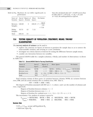
![329
ANALYSIS OF VARIANCE
Example 11.4: The following table gives the number of refrigerators sold by 4 salesmen in three months
May, June, and July:
Is there a significant difference in the sales made by the four salesmen? Is there a significant difference
in the sales made during different months? [Delhi Univ., M.Com., 1998, 2000]
Solution: Let us take the null hypothesis that there is no significant difference between sales made by the
four salesmen during different months. The given data are coded by subtracting 40 from each observation.
Calculations for a two-criteria—month and salesman—analysis of variance are shown in Table 11.7.
T = Sum of all observations in three samples of months = 48
CF = Correction factor =
2
T
n
=
2
(48)
12
= 192
SSTR = Sum of squares between salesmen (columns)
=
2 2 2 2
(15) (12) (18) (3)
3 3 3 3
+ + +
– 192
= (75 + 48 + 108 + 3) – 192 = 42
SSR = Sum of squares between months (rows)
=
2 2 2
(17) (29) (2)
4 4 4
+ +
– 192
= (72.25 + 210.25 + 1) – 192 = 91.5
SST = Total sum of squares
= (Σ x1
2
+ Σ x2
2
+ Σ x3
2
+ Σ x4
2
) – CF
= (137 + 80 + 164 + 27) – 192 = 216
SSE = SST – (SSC + SSR) = 216 – (42 + 91.5) = 82.5.
The total degrees of freedom are df = n – 1 = 12 – 1 = 11. So
dfc = c – 1 = 4 – 1 = 3, dfr = r – 1 = 3 – 1 = 2; df = (c – 1) (r – 1) = 3 × 2 = 6.
Thus, MSTR = SSTR/(c – 1) = 42/3 = 14
MSR = SSR/(r –1) = 91.5/2 = 45.75
MSE = SSE/(c – 1) (r – 1)=82.5/6=13.75.
The ANOVA table is shown in Table 11.8.
Table 11.7 Two-way ANOVA Table
Month Salesman Row
A(x1) x1
2
B(x2) x2
2
C(x3) x3
2
D(x4) x4
2
Sum
May 10 100 0 0 8 64 –1 1 17
June 6 36 8 64 10 100 5 25 29
July –1 01 4 16 0 0 –1 1 2
Column sum 15 137 12 80 18 164 3 27 48
Month Salesman
A B C D
May 50 40 48 39
June 46 48 50 45
July 39 44 40 39](https://image.slidesharecdn.com/businessstatisticsproblemsandsolutions-230910073954-6d42a210/85/Business-Statistics_-Problems-and-Solutions-pdf-343-320.jpg)
![BUSINESS STATISTICS: PROBLEMS AND SOLUTIONS
330
(a) The table value of F = 4.75 for df1 = 3, df2 = 6, and α = 0.05. Since the calculated value of Ftreatment
= 1.018 is less than its table value, the null hypothesis is accepted. Hence we conclude that the sales
made by the salesmen do not differ significantly.
(b) The table value of F=5.14 for df1= 2, df2 = 6, and α = 0.05. Since the calculated value of Fblock =
3.327 is less than its table value, the null hypothesis is accepted. Hence we conclude that sales made
during different months do not differ significantly.
Example 11.5: To study the performance of three detergents and three different water temperatures, the
following ‘whiteness’ readings were obtained with specially designed equipment:
Perform a two-way analysis of variance, using 5 per cent level of significance.
[Osmania Univ., MBA, 1998]
Solution: Let us take the null hypothesis that there is no significant difference in the performance of
three detergents due to water temperature and vice versa. The data are coded by subtracting 50 from each
observation. The data in coded form are shown in Table 11.9.
T = Sum of all observations in three samples of detergents = 56
CF = Correction factor =
2
T
n
=
2
(56)
9
= 348.44
SSTR = Sum of squares between detergents (columns)
=
2 2 2
(10) (3) (43)
3 3 3
+ +
– CF = 33.33 + 3 + 616.33 – 348.44 = 304.22
Table 11.9 Coded Data
Water Detergents
Temperature A(x1) x1
2
B(x2) x2
2
C(x3) x3
2
Row Sum
Cold water +7 49 +5 25 +17 289 29
Warm water –1 01 +2 04 +18 324 19
Hot water +4 16 –4 16 +8 64 8
Column sum 10 66 3 45 43 677 56
Table 11.8 Two-way ANOVA Table
Source of Sum of Squares Degrees of Mean Squares Variance Ratio
Variation Freedom
Between 42.0 3 14.00 Ftreatment = 14/13.75
salesmen = 1.018
Between 91.5 2 45.75 Fblock = 45.75/13.75
months = 3.327
Residual error 82.5 6 13.75
Total 216 11
Water Temperature Detergent A Detergent B Detergent C
Cold water 57 55 67
Warm water 49 52 68
Hot water 54 46 58](https://image.slidesharecdn.com/businessstatisticsproblemsandsolutions-230910073954-6d42a210/85/Business-Statistics_-Problems-and-Solutions-pdf-344-320.jpg)
![331
ANALYSIS OF VARIANCE
SSR = Sum of squares between water temperature (rows)
=
2 2 2
(29) (19) (8)
3 3 3
+ +
– CF
= (280.33 + 120.33 + 21.33) – 348.44 = 73.55
SST = Total sum of squares
= (Σ x1
2
+ Σ x2
2
+ Σ x3
2
) – CF
= (66 + 45 + 677) – 348.44 = 439.56
SSE = SST – (SSC + SSR)
= 439.56 – (304.22 + 73.55) = 61.79.
Thus, MSTR = SSTR /(c – 1) = 304.22/2 = 152.11;
MSR = SSR /(r – 1) = 73.55/2 = 36.775;
MSE = SSE/(c – 1) (r – 1) = 61.79/4 = 15.447.
(a) Since calculated value of Ftreatment = 9.847 at df1 = 2, df2 = 4, and α = 0.05 is greater than its table
value F = 6.94, the null hypothesis is rejected (Table 11.10). Hence we conclude that there is significant
difference between the performance of the three detergents.
(b) Since the calculated value of Fblock = 2.380 at df1 = 2, df2 = 4, and α = 0.05 is less than its table value
F = 6.94, the null hypothesis is accepted. Hence we conclude that the water temperature does not
make a significant difference in the performance of the detergent.
Example 11.6: Kerala Traders Co. Ltd. wishes to test whether its three salesmen A, B, and C tend to
make (in Rs.) sales of the same size of whether they differ in their selling ability as measured by the average
size of their sales. During the last week there have been 14 sales calls – A made 5 calls, B made 4 calls, and
C made 5 calls. Following are the weekly sales record of the three salesmen:
A B C
300 600 700
400 300 300
300 300 400
500 400 600
0 — 500
Perform the analysis of variance and draw you conclusions.
[Madras Univ., M.Com., 1996; Madurai Kamaraj, M.Com., 1996]
Table 11.10 Two-way ANOVA Table
Source of Sum of Squares Degree of Mean Squares Variance Ratio
Variation Freedom
Between detergents 304.22 2 152.110 Ftreatment = 152.11/15.447
(columns) = 9.847
Between temp. 73.55 2 36.775 Fblock = 36.775/15.447
(rows) = 2.380
Residual error 61.79 4 15.447
Total 439.56 8](https://image.slidesharecdn.com/businessstatisticsproblemsandsolutions-230910073954-6d42a210/85/Business-Statistics_-Problems-and-Solutions-pdf-345-320.jpg)
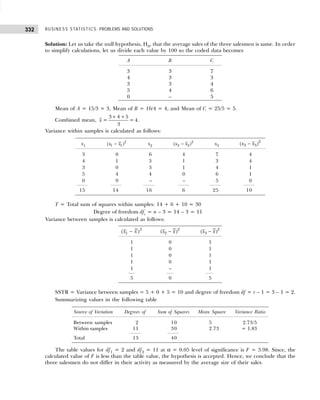
![333
ANALYSIS OF VARIANCE
Example 11.7: The following table gives the number of units of production per day turned out by four
different types of machines :
Employee Types of Machines
M1 M2 M3 M4
E1 40 36 45 30
E2 38 42 50 41
E3 36 30 48 35
E4 46 47 52 44
Using analysis of variance (a) test the hypothesis that the mean production is the same for the four
machines and (b) test the hypothesis that the employees do not differ with respect to mean productivity.
[Osmania Univ., M.Com., 1999]
Solution: Let us take the hypothesis that (a) the mean production does not differ for the four machines
and (b) the employees do not differ with respect to mean productivity.
Subtracting a common figure 40 from each observation. The calculations with coded data are as given
below:
Employees Machines
M1 M2 M3 M4 Total
E1 0 –4 5 –10 –9
E2 –2 2 10 1 11
E3 –4 –10 8 –5 –11
E4 6 7 12 4 29
0 –5 35 –10 20
T = Sum of all the observations in four samples = 20
Correction factor, CF =
2 2
(20)
= = 25
16
T
n
SSRT = Sum of squares between the samples
=
2
2 2 2
2
1 3 4
1 2 3 4
)
) ) )
x
x x x
CF
n n n n
(Σ
(Σ (Σ (Σ
+ + + −
=
2 2 2 2
(0) ( 5) ( 35) ( 10)
25
4 4 4 4
− − −
+ + + −
= 0 + 6.25 + 306.25 + 25 – 25 = 312.5
Sum of squares between employees:
=
2 2 2 2
( 9) (11) ( 11) (29)
4 4 4 4
CF
− −
+ + + −
= 20.25 + 30.25 + 30.25 + 210.25 – 25 = 266
Total sum of squares, SST = {[(0)2
+ (–2)2
+ (–4)2
+ (6)2
] + [(–4)2
+ (2)2
+ (–10)2
+ (7)2
]
+ [(5)2
+ (10)2
+ (8)2
+ (12)2
] + [(–10)2
+ (1)2
(–5)2
+ (4)2
]} – CF
= (0 + 4 + 16 + 36) + (16 + 4 + 100 + 49) + (25 + 100 + 64 + 144)
+ (100 + 1 + 25 + 16) – 25 = 675](https://image.slidesharecdn.com/businessstatisticsproblemsandsolutions-230910073954-6d42a210/85/Business-Statistics_-Problems-and-Solutions-pdf-347-320.jpg)
![BUSINESS STATISTICS: PROBLEMS AND SOLUTIONS
334
Degree of freedom, df = r – 1 = 4 – 1 = 3, df = 4 – 1 = 3, df = (r – 1)(c – 1) = 3 × 3 = 9.
These values are summarized in Table 11.11.
Table 11.11 ANOVA Table
Sum of Squares Degree of Freedom Mean Squares F
Between columns 321.5 3 104.17
104.17
= 9.72
10.72
Between rows 266.0 3 88.67
88.67
= 8.27
10.72
Residual error 96.5 9 10.72
Total 675.0 15
The table values of F0.05 = 3.86 for dfc = 3 and df = 9 and F0.05 = 3.86 for dfr = 3 and df = 9 at
α = 0.05 level of significance. Since the calculated values of F are more than its critical value, the
hypothesis is rejected. Hence the mean production is not the same for the four machines. Also, employees
differ with respect to mean productivity.
S e l f-P r a c t i c e P r o b l e m s 11B
11.6 A tea company appoints four salesmen A, B, C, and D,
and observes their sales in three seasons—summer,
winter, and monsoon. The figures (in lakhs) are given
in the following table:
Season Salesman
A B C D Total
Summer 36 36 21 35 128
Winter 28 29 31 32 120
Monsoon 26 28 29 29 112
Total 90 93 81 96 360
(a) Do the salesmen significantly differ in performance?
(b) Is there significant difference between the seasons?
[Calcutta Univ., M.Com., 1996; Calcutta Univ., M.Com., 1998]
11.7 Perform a two-way ANOVA on the data given below:
Plots of Treatment
Land A B C D
1 38 40 41 39
2 45 42 49 36
3 40 38 42 42
Use the coding method for subtracting 40 from the
given numbers. [CA, May, 1996]
11.8 The following data represent the production per day
turned out by 5 different workers using 4 different
types of machines:
Workers Machine Type
A B C D
1 44 38 47 36
2 46 40 52 43
3 34 36 44 32
4 43 38 46 33
5 38 42 49 39
(a) Test whether the mean productivity is the same for
the different machine types.
(b) Test whether the 5 men differ with respect to mean
productivity. [Madras Univ., M.Com., 1997]
11.9 The following table gives the number of units of
production per day turned out by four different types
of machines:
Employees Type of Machine
M1 M2 M3 M4
E1 40 36 45 30
E2 38 42 50 41
E3 36 30 48 35
E4 46 47 52 44
Using analysis of variance (a) test the hypothesis that
the mean production is same for four machines and
(b) test the hypothesis that the employees do not differ
with respect to mean productivity.
[Osmania Univ., M.Com., 1999]](https://image.slidesharecdn.com/businessstatisticsproblemsandsolutions-230910073954-6d42a210/85/Business-Statistics_-Problems-and-Solutions-pdf-348-320.jpg)
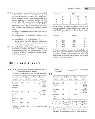
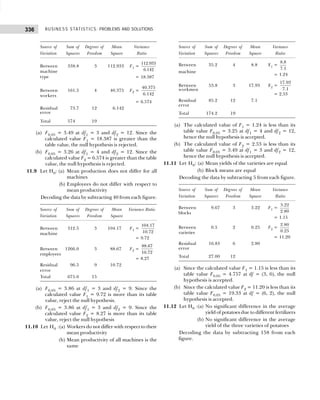
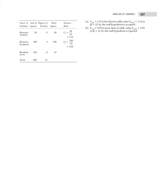
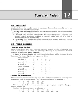
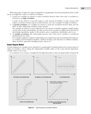
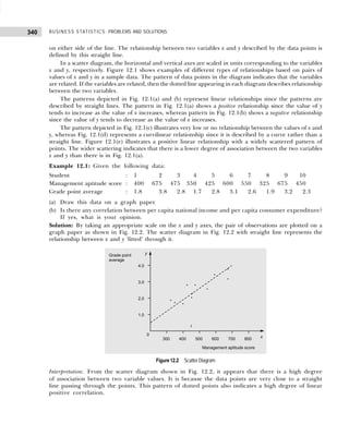
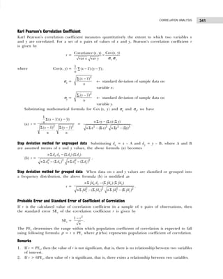
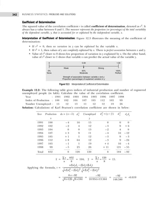
![343
CORRELATION ANALYSIS
Interpretation: Since coefficient of correlation r = –0.619 is moderately negative, it indicates that
there is a moderately large inverse correlation between the two variables. Hence, we conclude that
as the production index increases, the number of unemployed decreases and vice versa.
Example 12.3: The following table gives the distribution of items of production and also the
relatively defective items among them, according to size groups. Find the correlation coefficient
between size and defect in quality.
Size group : 15–16 16–17 17–18 18–19 19–20 20–21
No. of items : 200 270 340 360 400 300
No. of defective items : 150 162 170 180 180 114
[Delhi Univ., B.Com., 1999]
Solution: Let group size be denoted by variable x and number of defective items by variable y.
Calculations for Karl Pearson’s correlation coefficient are shown below:
Substituting values in the formula of Karl Pearson’s correlation coefficient r, we have
r =
2 2 2 2
( ) ( )
( ) ( )
x y x y
x x y y
n d d d d
n d d n d d
Σ − Σ Σ
Σ − Σ Σ − Σ
=
2 2
6 106 3 18
6 19 (3) 6 894 (18)
× − − ×
× − × −
=
636 54
105 5040
− −
= –
690
727.46
= – 0.949
Interpretation: Since value of r is negative, and is moderately close to –1, statistical association
between x (size group) and y (per cent of defective items) is moderate and negative, we conclude
that when size of the group increases, the number of defective items decreases and vice versa.
Example 12.4: The following data relate to age of employees and the number of days they reported
sick in a month.
Employees : 1 2 3 4 5 6 7 8 9 10
Age : 30 32 35 40 48 50 52 55 57 61
Sick days : 1 0 2 5 2 4 6 5 7 8
Calculate Karl Pearson’s coefficient of correlation and interpret it.
Solution: Let age and sick days be represented by variables x and y, respectively. Calculations for
value of correlation coefficient are shown below:
Size Mid-value dx = m – 17.5 d x
2 Per cent of dy = y – 50 d y
2
dxdy
Group m Defective Items
15–16 15.5 –2 4 75 +25 625 –50
16–17 16.5 –1 1 60 +10 100 –10
17–18 17.5 0 0 50 0 0 0
18–19 18.5 +1 1 50 0 0 0
19–20 19.5 +2 4 45 –5 25 – 10
20–21 20.5 +3 9 38 –12 144 –36
3 19 18 894 –106](https://image.slidesharecdn.com/businessstatisticsproblemsandsolutions-230910073954-6d42a210/85/Business-Statistics_-Problems-and-Solutions-pdf-357-320.jpg)
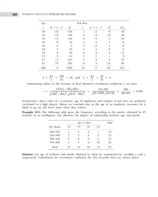
![345
CORRELATION ANALYSIS
where dx = x – 19, dy = (m – 275)/50.
Substituting values in the formula of Karl Pearson’s correlation coefficient, we have
r =
2 2 2 2
( ) ( )
( ) ( )
x y x y
x x y y
n fd d fd fd
n fd fd n fd fd
Σ − Σ Σ
Σ − Σ Σ − Σ
=
2 2
67 66 46 52
67 102 (46) 67 116 (52)
× − ×
× − × −
=
4422 2392
6834 2116 7772 2704
−
− −
=
2030
4718 5068
=
2030
68.688 71.19
×
= 0.415.
Interpretation: Since the value of r is positive, age of students and marks obtained in an intelligence
test are positively correlated to the extent of 0.415. Hence, we conclude that as the age of students
increases, score of marks in intelligence test also increases.
Example 12.6: Calculate the coefficient of correlation from the following bivariate frequency distribution:
[Delhi Univ., MBA, 1997]
Age in years
x 18 19 20 21
dx – 1 0 1 2 Total, f fdy fdy
2
fdxdy
y dy
200–250 – 1 4 0 –2 –2 11 –11 11 0
4 4 2 1
250–300 0 0 0 0 0 14 0 0 0
3 5 4 2
300–350 1 –2 0 8 10 21 21 21 16
2 6 8 5
350–400 2 –2 0 12 40 21 42 84 50
1 4 6 10
Total, f 10 19 20 18 n = 67 Σ fdy Σ fdy
2
Σ fdxdy
= 52 = 116 = 66
fdx –10 0 20 36 Σ fdx
= 46
fdx
2
10 0 20 72 Σ fdx
2
= 102
fdxdy 0 0 18 48 Σ fdxdy
= 66
Sales Revenue Advertising Expenditure Total
(Rs. in lakh) (Rs. in ’000)
5–10 10–15 15–20 20–25
75–125 4 1 — — 5
125–175 7 6 2 1 16
175–225 1 3 4 2 10
225–275 1 1 3 4 9
Total 13 11 9 7 40](https://image.slidesharecdn.com/businessstatisticsproblemsandsolutions-230910073954-6d42a210/85/Business-Statistics_-Problems-and-Solutions-pdf-359-320.jpg)

![347
CORRELATION ANALYSIS
S e l f-P r a c t i c e P r o b l e m s 12A
12.1 Making use of the data summarized below, calculate
the coefficient of correlation.
Case x1 x2 Case x1 x2
A 10 9 E 12 11
B 6 4 F 13 13
C 9 6 G 11 8
D 10 9 H 9 4
12.2 Find the correlation coefficient by Karl Pearson’s
method between x and y and interpret its value.
x: 57 42 40 33 42 45 42 44 40 56 44 43
y: 10 60 30 41 29 27 27 19 18 19 31 29
12.3 Calculate the coefficient of correlation from the
following data:
x : 100 200 300 400 500 600 700
y : 130 150 160 180 100 110 130
12.4 Calculate the coefficient of correlation between x
and y from the following data and calculate the
probable errors. Assume 69 and 112 as the mean
value for x and y, respectively.
x : 178 189 199 160 150 179 168 161
y : 125 137 156 112 107 136 123 108
12.5 Find the coefficient of correlation from the following
data:
Obtain the correct value of correlation coefficient between x and y.
[MD Univ., M.Com., 1998; Kumaon Univ., MBA, 2000]
Solution: The corrected values for termed needed in the formula of Pearson’s correlation coefficient
are determined as follows:
Correct Σ x = 125 – (6 + 8 – 8 – 6) = 125
Correct Σ y = 100 – (14 + 6 – 12 – 8) = 100
Correct Σ x2
= 650 – {(6)2
+ (8)2
– (8)2
– (6)2
} = 650 – {36 + 64 – 64 – 36} = 650
Correct Σ y2
= 460 – {(14)2
+ (6)2
– (12)2
– (8)2
} = 460 – {196 + 36 – 144 – 64} = 436
Correct Σ xy = 508 – {(6×14) + (8×6) – (8×12) – (6 × 8)} = 508 – {84 – 48 – 96 – 48} = 520.
Applying the formula,
r =
2 2 2 2
( ) ( )
( ) ( )
n xy x y
n x x n y y
Σ − Σ Σ
Σ − Σ Σ − Σ
=
2 2
25 520 125 100
25 650 (125) 25 436 (100)
× − ×
× − × −
=
13,000 12,500
625 900
−
=
500
25 30
×
= 0.667.
Thus, the correct value of correlation coefficient between x and y is 0.667.
Cost : 39 65 62 90 82 75 25 98 36 78
Sales : 47 53 58 86 62 68 60 91 51 84
[Madras Univ., B.Com., 1997]
12.6 Calculate Karl Pearson’s coefficient of correlation
between age and playing habits from the data given
below. Also calculate the probable error and
comment on the value:
Age : 120 121 122 123 124 25
No. of students : 500 400 300 240 200 160
Regular players : 400 300 180 196 160 24
[HP Univ., MBA, 1997]
12.7 Find the coefficient of correlation between age and
the sum assured (in 1000 Rs.) from the following table:
Age Group Sum Assured (in Rs.)
( Years) 10 20 30 40 50
20–30 4 6 03 7 1
30–40 2 8 15 7 1
40–50 3 9 12 6 2
50–60 8 4 02 — —
[Delhi Univ., MBA, 1999]
12.8 Family income and its percentage spent on food in
the case of 100 families gave the following bivariate
frequency distribution. Calculate the coefficient of
correlation and interpret its value.](https://image.slidesharecdn.com/businessstatisticsproblemsandsolutions-230910073954-6d42a210/85/Business-Statistics_-Problems-and-Solutions-pdf-361-320.jpg)
![BUSINESS STATISTICS: PROBLEMS AND SOLUTIONS
348
City Area in Population No. of Deaths
Kilometres (in ’000)
A 150 30 300
B 180 90 1440
C 100 40 560
D 060 42 840
E 120 72 1224
F 080 24 312
[Sukhadia Univ., B.Com., 1998]
12.10 The coefficient of correlation between two variables
x and y is 0.3. The covariance is 9. The variance of
x is 16. Find the standard deviation of y series.
Food
Monthly Family Income (Rs.)
Expenditure 2000 3000 4000 5000 6000
(in per cent) –3000 –4000 –5000 –6000 –7000
10–15 — — — 3 7
15–20 — 4 9 4 3
20–25 7 6 12 5 —
25–30 3 10 19 8 —
[Delhi Univ., MBA, 2000]
12.9 With the following data in 6 cities, calculate Pearson’s
coefficient of correlation between the density of
population and death rate:
Hints and Answers
12.1 1
x = 80/8 = 10, 2
x = 64/8 = 8;
r =
43
32 72
= 0.896
12.2 r = – 0.554 12.3 r = 0.997
12.4 r = 0.014 12.5 r = 0.780
12.6 r = 0.005 12.7 r = – 0.256
12.8 r = – 0.438 12.9 r = 0.988
12.10 Given σx = 16 = 4; r =
Cov( , )
x y
x y
σ σ
or 0.3 =
9
4 y
σ
or σy = 7.5.
12.3 SPEARMAN’S RANK CORRELATION COEFFICIENT
This method is applied to measure the association between two variables when only ordinal (or
rank) data are available. Mathematically, Spearman’s rank correlation coefficient is defined as
R = 1 –
2
2
6
( 1)
d
n n
Σ
−
where R = rank correlation coefficient;
R1 = rank of observations with respect to first variable;
R2 = rank of observations with respect to second variable;
d = R1 – R2, difference in a pair of ranks;
n = number of paired observations or individuals being ranked.
The number ‘6’ is placed in the formula as a scaling device, it ensures that the possible range
of R is from –1 to 1. While using this method we may come across three types of cases.
Case 1: When Ranks are Given
When observations in a data set are already arranged in a particular order (rank), take the
differences in pairs of observations to determine d. Square these differences and obtain the total
Σ d2
. Apply usual formula to calculate correlation coefficient.
Example 12.8: The coefficient of rank correlation between debenture prices and share prices is found
to be 0.143. If the sum of the squares of the differences in ranks is given to be 48, find the values
of n.](https://image.slidesharecdn.com/businessstatisticsproblemsandsolutions-230910073954-6d42a210/85/Business-Statistics_-Problems-and-Solutions-pdf-362-320.jpg)
![349
CORRELATION ANALYSIS
Solution: The formula for Spearman’s correlation coefficient is as follows:
R = 1 –
2
2
6
( 1)
d
n n
Σ
−
.
Given R = 0.143, Σ d2
= 48, and n=7. Substituting values in the formula, we get
0.143 = 1 – 2
6 48
( 1)
n n
×
−
= 1 – 3
288
n n
−
0.143 (n3
– n) = (n3
– n) – 288
n3
– n – 336 = 0 or (n – 7) (n2
+ 7n + 48) = 0.
This implies that either n – 7 = 0, that is, n = 7 or n2
+ 7n + 48 = 0. But n2
+ 7n + 48 = 0
on simplification gives undesirable value of n because its discriminant b2
– 4ac is negative. Hence,
n = 7.
Example 12.9: The ranks of 15 students in two subjects A and B are given below. The two numbers
within brackets denote the ranks of a student in A and B subjects respectively.
(1, 10), (2, 7), (3, 2), (4, 6), (5, 4), (6, 8), (7, 3), (8, 1),
(9, 11), (10, 15), (11, 9), (12, 5), (13, 14), (14, 12), (15, 13)
Find Spearman’s rank correlation coefficient. [Sukhadia Univ., MBA, 1998]
Solution: Since ranks of students with respect to their performance in two subjects are given,
calculations for rank correlation coefficient are shown below:
Apply the formula, R = 1 –
2
3
6 d
n n
Σ
Σ
−
= 1 – 2
6 272
15[(15) 1]
×
−
= 1 –
1632
3360
= 1 – 0.4857 = 0.5143.
The result shows a moderate degree of positive correlation between performance of students
in two subjects.
Rank in A Rank in B Difference d2
R1 R2 d = R1 – R2
1 10 –9 81
2 7 –5 25
3 2 1 1
4 6 –2 4
5 4 1 1
6 8 –2 4
7 3 4 16
8 1 7 49
9 11 –2 4
10 15 –5 25
11 9 2 4
12 5 7 49
13 14 –1 1
14 12 2 4
15 13 2 4
272](https://image.slidesharecdn.com/businessstatisticsproblemsandsolutions-230910073954-6d42a210/85/Business-Statistics_-Problems-and-Solutions-pdf-363-320.jpg)
![BUSINESS STATISTICS: PROBLEMS AND SOLUTIONS
350
Example 12.10: An office has 12 clerks. The long-serving clerks feel that they should have a
seniority increment based on length of service built into their salary structure. An assessment of
their efficiency by their departmental manager and the personnel department produces a ranking
of efficiency. This is shown below together with a ranking of their length of service.
Ranking according
to length of service : 1 2 3 4 5 6 7 8 9 10 11 12
Ranking according
to efficiency : 2 3 5 1 9 10 11 12 8 7 6 4
Do the data support the clerks’ claim for seniority increment? [Sukhadia Univ., MBA, 1991]
Solution: Since ranks are already given, calculations for rank correlation coefficient are shown
below:
Applying the formula, R = 1 –
2
2
6
( 1)
d
n n
Σ
−
= 1 –
6 178
12(144 1)
×
−
= 1 –
1068
1716
= 0.378.
The result shows a low degree of positive correlation between length of service and efficiency,
the claim of the clerks for a seniority increment based on length of service is not justified.
Example 12.11: Ten competitors in a beauty contest are ranked by three judges in the following
order:
Judge 1: 1 6 5 10 3 2 4 9 7 8
Judge 2: 3 5 8 4 7 10 2 1 6 9
Judge 3: 6 4 9 8 1 2 3 10 5 7
Use the rank correlation coefficient to determine which pair of judges has the nearest approach
to common tastes in beauty. [MD Univ., MBA, 1996]
Solution: The pair of judges who have the nearest approach to common taste in beauty can be
obtained in 3
C2 = 3 ways as follows:
(i) Judge 1 and Judge 2
(ii) Judge 2 and Judge 3
(iii) Judge 3 and Judge 1
Rank According to Rank According Difference d2
Length of Service to Efficiency d = R1 – R2
R1 R2
1 2 –1 1
2 3 –1 1
3 5 –2 4
4 1 3 9
5 9 –4 16
6 10 –4 16
7 11 –4 16
8 12 –4 16
9 8 1 1
10 7 3 9
11 6 5 25
12 4 8 64
178](https://image.slidesharecdn.com/businessstatisticsproblemsandsolutions-230910073954-6d42a210/85/Business-Statistics_-Problems-and-Solutions-pdf-364-320.jpg)
![351
CORRELATION ANALYSIS
Calculations for comparing their ranking are shown below:
Applying the formula,
R12 = 1 –
2
2
6
( 1)
d
n n
Σ
−
= 1 –
6 200
10(100 1)
×
−
= 1 –
1200
990
= – 0.212
R23 = 1 –
2
2
6
( 1)
d
n n
Σ
−
= 1 –
6 214
10(100 1)
×
−
= 1 –
1284
990
= – 0.297
R13 = 1 –
2
2
6
( 1)
d
n n
Σ
−
= 1 –
6 60
10(100 1)
×
−
= 1 –
360
990
= 0.636.
Since the correlation coefficient R13 = 0.636 is largest, Judges 1 and 3 have nearest approach to
common tastes in beauty.
Case 2: When Ranks are not Given
When pairs of observations in the data set are not ranked as in Case 1, the ranks are assigned by
taking either the highest value or the lowest value as 1 for both the variable’s values.
Example 12.12: Quotations of index numbers of security prices of a certain joint stock company
are given below:
Using the rank correlation method, determine the relationship between debenture prices and
share prices. [Calicut Univ., B.Com., 1997]
Judge 1 Judge 2 Judge 3 d2
= (R1 – R2)2
d2
= (R2 – R3)2
d2
= (R3 – R1)2
R1 R2 R3
1 3 6 4 9 25
6 5 4 1 1 4
5 8 9 9 1 16
10 4 8 36 16 4
3 7 1 16 36 4
2 10 2 64 64 0
4 2 3 4 1 1
9 1 10 64 81 1
7 6 5 1 1 4
8 9 7 1 4 1
200 214 60
Year Debenture Price Share Price
1 97.8 73.2
2 99.2 85.8
3 98.8 78.9
4 98.3 75.8
5 98.4 77.2
6 96.7 87.2
7 97.1 83.8](https://image.slidesharecdn.com/businessstatisticsproblemsandsolutions-230910073954-6d42a210/85/Business-Statistics_-Problems-and-Solutions-pdf-365-320.jpg)
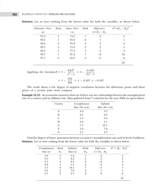
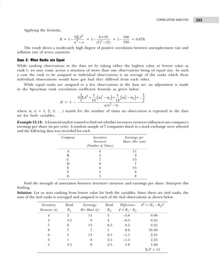
![BUSINESS STATISTICS: PROBLEMS AND SOLUTIONS
354
It may be noted that a value 5 of variable x is repeated twice (m1 = 2) and values 8 and 13 of variable
y are also reperated twice, so m2 = 2 and m3 = 2. Applying the formula,
R =
{ }
2 3 3 3
1 1 2 2 3 3
2
1 1 1
6 ( ) ( ) ( )
12 12 12
1
( 1)
d m m m m m m
n n
+ − + − + −
∑
−
−
= 1 –
{ }
3 3 3
1 1 1
6 51 (2 2) (2 2) (2 2)
12 12 12
7(49 1)
+ − + − + −
−
=
6{51 0.5 0.5 0.5}
1
336
+ + +
− = 1 – 0.9375 = 0.0625.
The result shows a very week positive association between inventory turnover and earnings per share.
Example 12.15: Obtain the rank correlation coefficient between the variables x and y from the
following pairs of observed values.
x : 50 55 65 50 55 60 50 65 70 75
y : 110 110 115 125 140 115 130 120 115 160
[Mangalore Univ., B.Com., 1997]
Solution: Let us start ranking from lowest value for both the variables. Moreover, certain observations in
both sets of data are repeated, the ranking is done in accordance with suitable average value as shown below.
It may be noted that for variable x, 50 is repeated thrice (m1 = 3), 55 is repeated twice (m2 =
2), and 65 is repeated twice (m3 = 2). Also for variable y, 110 is repeated twice (m4 = 2) and 115
is repeated thrice (m5 = 3). Applying the formula,
R = 1 –
{ }
2 3 3 3 3 3
1 1 2 2 3 3 4 4 5 5
2
1 1 1 1 1
6 ( ) ( ) ( ) ( ) ( )
12 12 12 12 12
( 1)
d m m m m m m m m m m
n n
Σ + − + − + − + − + −
−
R = 1 –
{ }
3 3 3 3 3
1 1 1 1 1
6 134 (3 3) (2 2) (2 2) (2 2) (3 3)
12 12 12 12 12
10(100 1)
+ − + − + − + − + −
−
= 1 –
6 [134 2 0.5 0.5 0.5 2]
990
+ + + + +
= 1 –
6 139.5
990
×
= 1 –
837
990
= 1 – 0.845 = 0.155.
The result shows a weak positive association between variables x and y.
Variable Rank Variable Rank Difference d2
= (R1 – R2)2
x R1 y R2 d = R1 – R2
50 2 110 1.5 0.5 0.25
55 4.5 110 1.5 3.0 9.00
65 7.5 115 4 3.5 12.25
50 2 125 7 –5.0 25.00
55 4.5 140 9 –4.5 20.25
60 6 115 4 2.0 4.00
50 2 130 8 –6.0 36.00
65 7.5 120 6 1.5 2.25
70 9 115 4 5.0 25.00
75 10 160 10 0.0 00.00
Σ d2
= 134.00](https://image.slidesharecdn.com/businessstatisticsproblemsandsolutions-230910073954-6d42a210/85/Business-Statistics_-Problems-and-Solutions-pdf-368-320.jpg)
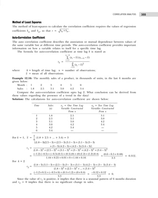
![BUSINESS STATISTICS: PROBLEMS AND SOLUTIONS
356
S e l f-P r a c t i c e P r o b l e m s 12B
12.11 The coefficient of rank correlation of the marks
obtained by 10 students in statistics and accountancy
was found to be 0.2. It was later discovered that
the difference in ranks in two subjects obtained by
one of the students was wrongly taken as 9 instead
of 7. Find the correct coefficient of rank correlation.
[Delhi Univ., B.Com., 1996]
12.12 The ranking of 10 students in accordance with their
performance in two subjects A and B are as follows:
A: 6 5 3 10 2 4 9 7 8 1
B: 3 8 4 9 1 6 10 7 5 2
Calculate the rank correlation coefficient and
comment on its value.
12.13 Calculate Spearman’s coefficient of correlation
between marks assigned to 10 students by judges
x and y in a certain competitive test as shown below:
Student Marks by Judge x Marks by Judge y
1 52 65
2 53 68
3 42 43
4 60 38
5 45 77
6 41 48
7 37 35
8 38 30
9 25 25
10 27 50
12.14 An examination of eight applicants for a clerical
post was taken by a firm. From the marks obtained
by the applicants in the accountancy and statistics
papers, compute the rank correlation coefficient.
Applicant : A B C D E F G H
Marks in
accountancy: 15 20 28 12 40 60 20 80
Marks in
statistics : 40 30 50 30 20 10 30 60
12.15 Seven methods of imparting business education were
ranked by the MBA students of two universities as
follows:
Method of Teaching : 1 2 3 4 5 6 7
Rank by students
of Univ. A : 2 1 5 3 4 7 6
Rank by students
of Univ. B : 1 3 2 4 7 5 6
Calculate the rank correlation coefficient and
comment on its value.
12.16 An investigator collected the following data with
respect to the socio-economic status and severity of
respiratory illness.
Patient : 1 2 3 4 5 6 7 8
Socio-economic
status (rank) : 6 7 2 3 5 4 1 8
Severity of illness
(rank) : 5 8 4 3 7 1 2 6
Calculate the rank correlation coefficient and
comment on its value.
12.17 You are given the following data of marks obtained
by 11 students in statistics in two tests, one before
and an other after special coaching:
First Test Second Test
(Before Coaching) (After Coaching)
23 24
20 19
19 22
21 18
18 20
20 22
18 20
20 22
18 20
17 20
23 23
16 20
19 17
Do the marks indicate that the special coaching has
benefited the students? [Delhi Univ., M.Com., 1989]
12.18 Two departmental managers ranked a few trainees
according to their perceived abilities. The ranking
are given below:
Trainee : A B C D E F G H I J
Manager A : 1 09 6 2 5 8 7 3 10 4
Manager B : 3 10 8 1 7 5 6 2 09 4
Calculate an appropriate correlation coefficient to
measure the consistency in the ranking.
12.19 In an office some keyboard operators, who were
already ranked on their speed, were also ranked on
accuracy by their supervisor. The results were as
follows:](https://image.slidesharecdn.com/businessstatisticsproblemsandsolutions-230910073954-6d42a210/85/Business-Statistics_-Problems-and-Solutions-pdf-370-320.jpg)
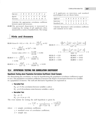
![BUSINESS STATISTICS: PROBLEMS AND SOLUTIONS
358
The t-test statistic follows t-distribution with n – 2 degrees of freedom. If the sample size is
large, then the standard error of correlation coefficient is given by sr = (1 – r2
)/ n .
Decision Rule: The calculated value of t-test statistic is compared with its critical (or table) value
at n – 2 degrees of freedom and level of significance α to arrive at a decision as follows:
Example 12.17: A random sample of 27 pairs of observations from a normal population gives a
correlation coefficient of 0.42. Is it likely that the variables in the population are uncorrelated?
[Delhi Univ., M.Com., 1997]
Solution: Let us take the null hypothesis that there is no significant difference in the sample and
population correlation coefficients, that is,
H0 : ρ = 0 and H1 : ρ ≠ 0
Given n = 27, df = n – 2 = 25, r = 0.42. Applying t-test statistic to test the null hypothesis, H0,
t =
r
r
s
− ρ
=
2
(1 ) ( 2)
r
r n
− −
=
( )
− −
2
0.42
{1 0.42 } (27 2)
=
0.42
0.908 /5
= 2.312.
Since the calculated value of t = 2.312 is more than the table value t = 1.708 at α = 0.05 and
df = 25, the null hypothesis is rejected. Hence, it is likely that the variables in the population are not
correlated.
Example 12.18: How many pairs of observations must be included in a sample so that an observed
correlation coefficient of value 0.42 shall have a calculated value of t greater than 2.72?
Solution: Given r = 0.42, t = 2.72. Applying t-test statistic, we get
2
(1 ) /( 2)
r
r n
− −
= t or r2
× 2
2
1
n
r
−
−
= t2
(0.42)2
× 2
( 2)
1 (0.42)
n −
−
= (2.72)2
n – 2 =
2 2
2
(2.72) [1 (0.42) ]
(0.42)
−
=
7.3984(0.8236)
0.1764
=
6.0933
0.1764
= 34.542
n = 2 + 34.542 = 36.542 ≅ 37.
Hence, the sample size should be of 37 pairs of observations.
Example 12.19: To study the correlation between the stature of father and son, a sample of 1600
is taken from the universe of fathers and sons. The sample study gives the correlation between the
two to be 0.80. Within what limits does it hold true for the universe?
Solution: Since the sample size is large, the standard error of the correlation coefficient is given
by
SEr =
2
1 r
n
−
.
One-tailed Test Two-tailed Test
Reject H0 Reject H0 if tcal > tα/2, n – 2
if tcal > tα, n–2 or tcal < – tα.
Otherwise accept H0 Otherwise accept H0](https://image.slidesharecdn.com/businessstatisticsproblemsandsolutions-230910073954-6d42a210/85/Business-Statistics_-Problems-and-Solutions-pdf-372-320.jpg)
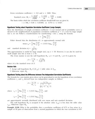
![BUSINESS STATISTICS: PROBLEMS AND SOLUTIONS
360
Solution: Given r = 0.75, n = 30, and ρ = 0.9. Applying Fisher’s z-transformation, we get
z = 1.1513 log10
1
1
r
r
+
−
= 1.1513 log10
1.75
0.25
= 1.1513 [log10 1.75 – log10 0.25]
= 1.1513 (0.24304 – 1 39794
. ) = 0.973.
The distribution of z is normal around the true population correlation value ρ = 0.9. Therefore,
Mean zρ = 1.1513 log10
1
1
+
−
ρ
ρ
= 1.1513 log10
1 0.90
1 0.90
+
−
= 1.1513 log10
1.90
0.10
= 1.1513 [log10 1.90 – log10 0.10] = 1.1513 (0.27875 + 1) = 1.47.
Thus, the Z-test statistic is given by
Z =
| |
z
z z
− ρ
σ
=
| |
1 3
z z
n
−
−
ρ
=
|0.973 1.47|
1 30 3
−
−
= 0.498 × 5.196 = 2.59
Hence, ρ (r ≤ 0.75) = P [Z ≤ 2.59] = 1 – 0.9952 = 0.0048.
Example 12.21: Test the significance of the correlation r = 0.5 from a sample of size 18 against
hypothesized population correlation ρ = 0.70.
Solution: Let us take the null hypothesis that the difference is not significant, that is,
H0 : ρ = 0.70 and H1 : ρ ≠ 0.70
Given n = 18, r = 0.5. Applying z-transformation, we have
z = 1.1513 log10
1
1
r
r
+
−
= 1.1513 log10
1 0.5
1 0.5
+
−
= 1.1513 log10
1.50
0.5
= 1.1513 log10 3
= 1.1513 (0.4771) = 0.5492
and mean zρ = 1.1513 log10
1
1
+
−
ρ
ρ
= 1.1513 log10
1 0.70
1 0.70
+
−
= 1.1513 log10
1.70
0.30
= 1.1513 log10 5.67
= 1.1513 (0.7536) = 0.8676.
Applying Z-test statistic, we get
Z =
| |
z
z z
− ρ
σ
=
| |
1 3
z z
n
−
−
ρ
= |z – zρ| − 3
n
= | 0.5492 – 0.8676 | 15 = 0.3184 (3.872) = 1.233.
Since calculated value of Zcal = 1.233 is less than its table value Zα./2 = 1.96 at 5 per cent
significance level, the null hypothesis is accepted. Hence, we conclude that the difference (if any)
is due to sampling error.
Example 12.22: Two independent samples of size 23 and 21 pairs of observations were analysed
and their coefficient of correlation was found as 0.5 and 0.8, respectively. Do these values differ
significantly?
Solution: Let us take the null hypothesis that two values do not differ significantly, that is, the
samples are drawn from the same population.](https://image.slidesharecdn.com/businessstatisticsproblemsandsolutions-230910073954-6d42a210/85/Business-Statistics_-Problems-and-Solutions-pdf-374-320.jpg)
![361
CORRELATION ANALYSIS
Given n1 = 23, r1 = 0.5; n2 = 28, r2 = 0.8. Applying Z-test statistic as follows,
Z =
1 2
1 2
z z
z z
−
−
σ
; z1 = 1.1513 log10
1
1
1
1
r
r
+
−
= 1.1513 log10
1 0.5
1 0.5
+
−
=
1 2
1 2
1 1
3 3
z z
n n
−
+
− −
=
0.55 1.10
1 1
20 25
−
+
= 1.1513 log10 3 = 0.55
=
0.55
0.30
= 1.833 z2 = 1.1513 log10
2
2
1
1
r
r
+
−
= 1.1513 log10
1 0.8
1 0.8
+
−
= 1.1513 log10 9 = 1.10.
Since the calculated value of Zcal = 1.833 is less than its table value Zα/2 = 1.96 at 5 per cent significance
level, the null hypothesis is accepted. Hence, the difference in correlation values is not significant.
12.5 MISCELLANEOUS SOLVED EXAMPLES
Example 12.23: Making use of the data summarized below, calculate the coefficient of correlation:
Case x1 x2 Case x1 x2
A 10 9 E 12 11
B 6 4 F 13 13
C 9 6 G 11 8
D 10 9 H 9 4
[Calicut Univ., B.Com., 2004]
Solution: Calculations required for coefficient of correlation are shown in the table below:
Case x1 dx = (x1 – 1
x ) dx
2
x2 dy = (x2 – 2
x ) dy
2
dx dy
A 10 0 0 9 +1 1 0
B 6 –4 16 4 –4 16 16
C 9 –1 1 6 –2 4 2
D 10 0 0 9 1 1 0
E 12 2 4 11 3 9 6
F 13 3 9 13 5 25 15
G 11 1 1 8 0 0 0
H 9 1 1 4 –4 16 4
N = 8 80 0 32 64 0 72 43
1
x = 1 80
= =10
8
x
N
Σ
and 2
x = 2 64
= =8
8
x
N
Σ
r12 =
2 2
x y
x y
d d
d d
Σ
Σ × Σ
=
43 43 43
= = =0.896
48
2304
32 72
×
.
Example 12.24: The following table gives indices of industrial production of registered unemployed (in
hundred thousand). Calculate the value of the coefficient so obtained.
Year : 1991 1992 1993 1994 1995 1996 1997 1998
Index of production : 100 102 104 107 105 112 103 99
Number unemployed : 15 12 13 11 12 12 19 26
[Garwhal Univ., M.A. (Eco.), 1998]](https://image.slidesharecdn.com/businessstatisticsproblemsandsolutions-230910073954-6d42a210/85/Business-Statistics_-Problems-and-Solutions-pdf-375-320.jpg)
![BUSINESS STATISTICS: PROBLEMS AND SOLUTIONS
362
Solution: Calculations required for Karl Pearson’s correlation coefficient are shown in the table below:
Year Production dx = (x – x ) 2
x
d Unemployed dy = (y – y) 2
y
d dx dy
1991 100 –4 16 15 0 0 0
1992 102 –2 4 12 –3 9 6
1993 104 0 0 13 –2 4 0
1994 107 3 9 11 –4 16 –12
1995 105 1 1 12 –3 9 –3
1996 112 8 64 12 –3 9 –24
1997 103 –1 1 19 4 16 –4
1998 99 –5 25 26 11 121 –55
832 0 120 120 0 184 –92
x = 2
832 120
= =104 and = =15
8 8
x y
y
N N
Σ Σ
=
r =
2 2
x y
x y
d d
d d
Σ
Σ Σ
=
92
= 0.619.
120 184
−
−
×
Example 12.25: Calculate the coefficient of correlation between x and y from the following data and
calculate probable error. Assume 69 and 112 as the mean value for x and y respectively.
x : 78 89 99 60 59 79 68 61
y : 125 137 156 112 107 136 123 108
[Punjab Univ., B.Com., 1997; HPU, B.Com., 1998]
Solution: Calculations required for Karl Perason’s correlation coefficient are shown in the table below:
x dx = (x – 69) 2
x
d y dy = (Y – 112) 2
y
d dxdy
78 +9 81 125 13 169 117
89 20 400 137 25 625 500
99 30 900 156 44 1936 1320
60 –9 81 112 0 0 0
59 –10 100 107 –5 25 50
79 10 100 136 24 576 240
68 –1 1 123 11 121 –11
61 –8 64 108 –4 16 32
593 41 1727 1004 108 3468 2248
Given A = 69 and B = 12 are the assumed mean of x and y series values. Applying the formula,
r =
2 2 2 2
( ) ( )
( ) ( )
x y x y
x x y y
N d d d d
N d d N d d
Σ − Σ Σ
Σ − Σ Σ − Σ
=
2 2
(8) (2248) (41) (108)
(8) (1727) (41) (8) (3468) (108)
−
− −
=
17984 4428
13816 1681 27744 11664
−
− −
=
13556 13556 13556
= = =0.97.
110.16 126.806 13968.95
12135 16080 ×
PEr =
2 2
1 1 (0.97)
0.6745 =0.6745
8
r
n
− −
=
0.6745 0.0591
0.014.
2.828
×
=](https://image.slidesharecdn.com/businessstatisticsproblemsandsolutions-230910073954-6d42a210/85/Business-Statistics_-Problems-and-Solutions-pdf-376-320.jpg)
![363
CORRELATION ANALYSIS
Example 12.26: The following table gives the frequency, according to groups of marks obtained by 67
students in an intelligence test. Measure the degree of relationship between age and intelligence test.
Test Marks
Age in Years (x)
Total
(y) 18 19 20 21
200–250 4 4 2 1 11
250–300 3 5 4 2 14
300–350 2 6 8 5 21
350–400 1 4 6 10 21
10 19 20 18
[Kurukshetra Univ., B.Com., 1996; Allahabad Univ., B.Com., 1999]
Solution: Calculations for coefficient of correlation are shown in the table below:
x
dx
18 19 20 21
dy –1 0 1 2 f fdy fdy
2
fdx dy
200–250 –1 +4 0 –2 –2 11 –11 11 0
4 4 2 1
250–300 0 0 0 0 0 14 0 0 0
3 5 4 2
300–350 1 –2 0 8 10 21 21 21 16
2 6 8 5
350–400 2 –2 0 12 40 21 42 84 50
1 4 6 10
Total –10 19 20 18 N = 67 52 116 66
fdx –10 0 20 36 46
fdx
2
10 0 20 72 102
fdx dy 0 0 18 48 66
r = 2 2 2 2
( ) ( )
x y x y
x x y y
N f d d f d f d
N f d f d N f d f d
Σ − Σ Σ
Σ − Σ Σ − Σ
=
2 2
67 66 46 52
67 102 (46) 67 116 (52)
× − ×
× − × −
=
4422 2392
6834 2116 7772 2704
−
− −
=
2030
4718 5068
=
2030
68.688 71.19
×
=
2030
= 0.415.
4889.899
Example 12.27: Calculate the coefficient of correlation from the following data by the Speaman’s Rank
difference method.
y](https://image.slidesharecdn.com/businessstatisticsproblemsandsolutions-230910073954-6d42a210/85/Business-Statistics_-Problems-and-Solutions-pdf-377-320.jpg)
![BUSINESS STATISTICS: PROBLEMS AND SOLUTIONS
364
Price of Price of Price of Price of
Tea (Rs.) Coffee (Rs.) Tea (Rs.) Coffee (Rs.)
75 120 60 110
88 134 80 140
95 150 81 142
70 115 50 100
[Agra Univ., B.Com., 1996]
Solution: Calculations for Spearman’s rank correlation coefficient are shown in the table below:
Price of Tea Rank Tea Price of Coffee Rank Coffee D2
= (R1 – R2)2
(Rs.) R1 (Rs.) R2
75 4 120 4 0
88 7 134 5 4
95 8 150 8 0
70 3 115 3 0
60 2 110 2 0
80 5 140 6 1
81 6 142 7 1
50 1 100 1 0
Σ D2
= 6
R =
2
3 3
6 6 6
1 =1
8 8
D
n n
Σ ×
− −
− −
=
36
1 =1 0.071=0.929.
512 8
− −
−
Example 12.28: Obtain the rank correlation coefficient between the variable X and Y from the following
pairs of observed values:
X : 50 55 65 50 55 60 50 65 70 75
Y : 110 110 115 125 140 115 130 120 115 160
[Mangalore Univ., B.Com., 1997]
Solution: To find rank correlation coefficient, rank various values as follows by considering lowest as
1 and next higher as 2.
X Rank X Y Rank Y D2
= (R1 – R2)2
R1 R2
50 2 110 1.5 0.25
55 4.5 110 1.5 9.00
65 7.5 115 4 12.25
50 2 125 7 25.00
55 4.5 140 9 20.25
60 6 115 4 4.00
50 2 130 8 36.00
65 7.5 120 6 2.25
70 9 115 4 25.00
75 10 160 10 00.00
134.00
It may be noted that in series X, 50 has repeated thrice (m1 = 3), 55 has been repeated twice (m2 = 2),
65 has been repeated twice (m3 = 2). In series Y, 110 has been repeated twice (m4 = 2) and 115 has thrice
(m5 = 3).](https://image.slidesharecdn.com/businessstatisticsproblemsandsolutions-230910073954-6d42a210/85/Business-Statistics_-Problems-and-Solutions-pdf-378-320.jpg)
![365
CORRELATION ANALYSIS
R = 1 –
2 3 3 3 3 3
1 1 2 2 3 3 4 4 5 5
3
1 1 1 1 1
6 ( ) ( ) ( ) ( ) ( )
12 12 12 12 12
D m m m m m m m m m m
n n
Σ + − + − + − + − + −
−
R = 1 –
3 3 3 3 3
3
1 1 1 1 1
6 134 (3 3) (2 2) (2 2) (2 2) (3 3)
12 12 12 12 12
10 10
+ − + − + − + − + −
−
=
6 (134 2 0.5 0.5 0.5 2)
1
990
+ + + + +
− = 6 (139.5) 837
1 =1 =1 845=0.155.
990 990
− − −
Example 12.29: Calculate Karl Pearson’s Coefficient of correlation between age and playing habits from
the data given below. Also calculate probable error and comment on the value :
Age : 20 21 22 23 24 25
No. of Students : 500 400 300 240 200 160
Regular Players : 400 300 180 96 60 24
[HPU, MBA, 1998; Kumaon Univ., MBA, 2001; Delhi Univ., MBA, 2006]
Solution: Calculations for Karl Pearson’s coefficient of correlation between age and percentage of regular
players are shown below:
Age dx = (x – 22) dx
2
No. of Regular Percentage of dy = (Y – 50) d2
y dx dy
(x) Students Players Regular
Player, y
20 –2 4 500 400 80 30 900 –60
21 –1 1 400 300 75 25 625 –25
22 0 0 300 180 60 10 100 0
23 1 1 240 96 40 –10 100 –10
24 2 4 200 60 30 –20 400 –40
25 3 9 160 24 15 –35 1225 –105
135 3 19 300 0 3350 –240
r =
2 2 2 2
( ) ( )
( ) ( )
x y x y
x x y y
N d d d d
N d d N d d
Σ − Σ Σ
Σ − Σ Σ − Σ
=
× − − ×
×
× − 2
6 240 (3 0)
6 3350
6 19 (3)
=
1440 1440
= = 0.991.
1452.756
105 20100
− −
−
×
PEr =
2
1
0.6745
r
N
−
=
0.6745 0.018
0.005.
2.449
×
=
Example 12.30: With the following data in 6 cities calculate the coefficient of correlation by Pearson’s
method between the density of population and death rate:
City Area (in km) Population (in ‘000) Number of Deaths
A 150 30 300
B 180 90 1440
C 100 40 560
D 60 42 840
E 120 72 1224
F 80 24 312
[Sukhadia Univ., B.Com., 1998]](https://image.slidesharecdn.com/businessstatisticsproblemsandsolutions-230910073954-6d42a210/85/Business-Statistics_-Problems-and-Solutions-pdf-379-320.jpg)
![BUSINESS STATISTICS: PROBLEMS AND SOLUTIONS
366
Solution: Calculating density of population (x) and death rate (y).
Density =
Population
Area
, and Death rate =
No. of Death
Population
×1000.
City Density (x – 450)/100 dx
2
Death rate (y – 15) dy
2
dx dy
(x) dx (y) dy
A 200 –2.5 6.25 10 –5 25 12.5
B 500 0.5 0.25 16 1 1 0.5
C 400 –0.5 0.25 14 –1 1 0.5
D 700 2.5 6.25 20 5 25 12.5
E 600 1.5 2.25 17 2 4 3.0
F 300 –1.5 2.25 13 –2 4 3.0
0 17.5 90 0 60 32
r =
2 2
32 32
= = =0.988.
32.404
17.5 60
x y
x y
d d
d d
Σ
×
Σ Σ
There is a high degree of positive correlation between density of population and death rate.
Example 12.31: The coefficient of rank correlation of the marks obtained by 10 students in statistics and
accountancy was found to be 0.2. It was later discovered that the difference in ranks in the two subjects
obtained by one of the students was wrongly taken as 9 instead of 7. Find the correct coefficient of rank
correlation. [Delhi Univ., B.Com.(H), 1992]
Solution: Given rank correlation, R = 0.2 and n = 10. Thus,
R =
2
3
6
1
D
n n
Σ
−
−
or 0.2 =
2
3
6
1
10 10
D
Σ
−
−
0.2 – 1.0 =
2
6
990
D
Σ
−
– 0.8 =
2
2
6
, i.e., =132.
990
D
D
Σ
Σ
Correct value of Σ D2
= 132 – (9)2
+ (7)2
= 132 – 81 + 49 = 100.
Correct R =
2
3
6
1
10 10
D
Σ
−
−
=
6×100
1 =1 0.606=0.394.
900
− −
Example 12.32: Compute Karl Pearson’s coefficient of correlation between per capita National Income
and per capita Consumer Expenditure from the data given below:
Years Per Capita National Income Per Capita Consumer
Expenditure
1988 249 237
1989 251 238
1990 248 236
1991 252 240
1992 258 245
1993 269 255
1994 271 254
1995 272 252
1996 280 258
1997 275 251
Also calculate probable error. [Bangalore Univ., B.Com., 1998]](https://image.slidesharecdn.com/businessstatisticsproblemsandsolutions-230910073954-6d42a210/85/Business-Statistics_-Problems-and-Solutions-pdf-380-320.jpg)
![367
CORRELATION ANALYSIS
Solution: Since the actual means of X and Y variable are not whole number, let us consider assumed
mean x = A = 260 and y = B = 240. Calculations for Karl Pearson’s correlation coefficient are shown
below:
Calculation of Karl Pearson’s Coefficient
x dx = (x – A) dx
2
y dy = (y – A) dy2
dx.dy
249 –11 121 237 –3 9 33
251 –9 81 238 –2 4 18
248 –12 144 236 –4 16 48
252 –8 64 240 0 0 0
258 –2 4 245 5 25 –10
269 9 81 255 15 225 135
271 11 121 254 14 196 154
272 12 144 252 12 144 144
280 20 400 258 18 324 360
275 15 225 251 11 121 165
2625 25 1385 2466 66 1064 1047
r =
2 2 2 2
( ) ( )
( ) ( )
x y x y
x x y y
n d d d d
n d d n d d
Σ − Σ Σ
Σ − Σ Σ − Σ
=
2 2
10 1047 25 66
10 1385 (25) 10 1064 (66)
× − ×
× − × −
=
882 882
= =0.967.
36.367 25.07 911.72
×
PEr =
2
1
0.6745
r
N
−
=
2
1 (0.967) 0.6745 0.065
0.6745 = =0.014.
3.162
10
− ×
Example 12.33: Given r = 0.8, Σ xy = 60, σy = 2.5, and Σ x2
= 90, find the number of items X and Y are
deviations from arithmetic mean. [Delhi Univ., B.Com.(H), 1998]
Solution: Given that Σ x2
= 90, r = 0.8, σy = 2.5, Σ xy = 60. Applying the formula to find number
of observations,
σx
2
= 2 2
1 1 90
( ) = =
x
x x d
n n n
Σ − Σ
r =
( ) ( )
=
x y
x y x y
d d
x x y y
n n
Σ
Σ − −
σ σ σ σ
or r2
=
2
2 2 2
( )
x y
x y
d d
n
Σ
σ σ
(0.8)2
=
2
2
(60) 3600
=
90 90 (6.25)
6.25 n
n
n
×
× ×
0.64 =
3600
562.5 n
0.64 × 562n = 3600 or 360n = 3600, i.e., n = 10.](https://image.slidesharecdn.com/businessstatisticsproblemsandsolutions-230910073954-6d42a210/85/Business-Statistics_-Problems-and-Solutions-pdf-381-320.jpg)
![BUSINESS STATISTICS: PROBLEMS AND SOLUTIONS
368
Example 12.34: Calculate Karl Pearson’s coefficient of correlation from the following data:
X 200–300 300–400 400–500 500–600 600–700
Y
10–15 — — — 3 7
15–20 — 4 9 4 3
20–25 7 6 12 5 —
25–30 3 10 19 8 —
[Delhi Univ., MBA, 2000]
Solution: Calculations for Karl Pearson’s coefficient of correlation are shown below:
X Series
dx
200–300 300–400 400–500 500–600 600–700
Y
m 250 350 450 550 650
Series m dy –2 –1 0 1 2 f fdy fdy
2
fdx dy
10–15 12.5 –1 – – – 3 7 10 –10 10 –17
0 0 0 –3 –14
15–20 17.5 0 – 4 9 4 3 20 0 0 0
0 0 0 0 0
20–25 22.5 1 7 6 12 5 – 30 30 30 –5
–14 –6 0 5 0
25–30 27.5 2 3 10 19 8 – 40 80 160 –16
–12 –20 0 16 0
Total 10 20 40 20 10 100 = N 100 200 –48
fdx –20 –20 0 20 20 0
fdx
2
40 20 0 20 40 120
fdx dy –26 –26 0 18 –14 –48
r =
2 2 2 2
( ) ( )
x y x y
x x y y
n d d d d
n f d f d n f d f d
Σ − Σ Σ
Σ − Σ Σ − Σ
=
2 2
100 ( 48) 0 100
100 (120) (0) 100 (200) (100)
− − ×
− −
=
4800 4800
= = 0.438.
10954
12000 10000
− −
−](https://image.slidesharecdn.com/businessstatisticsproblemsandsolutions-230910073954-6d42a210/85/Business-Statistics_-Problems-and-Solutions-pdf-382-320.jpg)
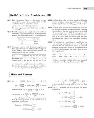
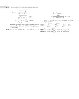
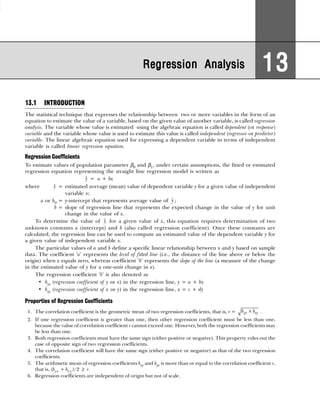
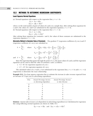
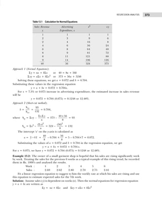
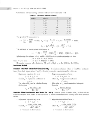
![375
REGRESSION ANALYSIS
dx = x – A; A is assumed mean of x dx = x – A; A is assumed mean
dx = = of x
dy = y – B; B is assumed mean of y dy = y – B; B is assumed mean
of y
Regression Coefficients in Terms of Correlation Coefficient If deviations are taken from actual mean values,
then the values of regression coefficients can be alternatively calculated as follows:
byx =
Σ − −
Σ − 2
( ) ( )
( )
x x y y
x x
bxy =
Σ − −
Σ − 2
( ) ( )
( )
x x y y
y y
= 2
Covariance( , )
x
x y
σ
=
y
x
r
σ
σ
. = 2
Covariance( , )
y
x y
σ
= x
y
r
σ
σ
.
Example 13.3: The following data relate to the scores obtained by 9 salesmen of a company in an intelligence
test and their weekly sales (in Rs. 1000’s):
Salesmen : A B C D E F G H I
Test scores : 50 60 50 60 80 50 80 40 70
Weekly sales : 30 60 40 50 60 30 70 50 60
(a) Obtain the regression equation of sales on intelligence test scores of the salesmen.
(b) If the intelligence test score of a salesman is 65, what would be his expected weekly sales.
[HP Univ., M.Com., 1996]
Solution: Assume weekly sales (y) as dependent variable and test scores (x) as independent variable.
Calculations for the following regression equation are shown in Table 13.3.
y – y = byx (x – x )
(a) x =
Σ x
n
=
540
9
= 60; y =
Σ y
n
=
450
9
= 50
byx = 2
( )( )
( )
x y x y
x x
d d d d
d d 2
Σ − Σ Σ
Σ − Σ
=
1200
1600
= 0.75.
Substituting values in the regression equation, we have
y – 50 = 0.75 (x – 60) or y = 5 + 0.75x.
For test score x = 65 of salesman, we have
y = 5 + 0.75 (65) = 53.75.
Hence, we conclude that the weekly sales is expected to be Rs. 53.75 (in Rs. 1000’s) for a test score of 65.
Table 13.3 Calculations for Regression Equation
Weekly dx = x – 60 dx
2
Test dy = y – 50 dy
2
dxdy
Sales, x Score, y
50 –10 100 30 –20 400 200
60 0 0 60 10 100 0
50 –10 100 40 –10 100 100
60 0 0 50 0 0 0
80 20 400 60 10 100 200
50 –10 100 30 –20 400 200
80 20 400 70 20 400 400
40 –20 400 50 0 0 0
70 10 100 60 10 100 100
540 0 1600 450 0 1600 1200](https://image.slidesharecdn.com/businessstatisticsproblemsandsolutions-230910073954-6d42a210/85/Business-Statistics_-Problems-and-Solutions-pdf-389-320.jpg)
![BUSINESS STATISTICS: PROBLEMS AND SOLUTIONS
376
Example 13.4: A company is introducing a job evaluation scheme in which all jobs are graded by points
for skill, responsibility, and so on. Monthly pay scales (Rs. in 1000’s) are then drawn up according to the
number of points allocated and other factors such as experience and local conditions. To date the company
has applied this scheme to 9 jobs:
Job : A B C D E F G H I
Points : 5 25 7 19 10 12 15 28 16
Pay (Rs.) : 3.0 5.0 3.25 6.5 5.5 5.6 6.0 7.2 6.1
(a) Find the least squares regression line for linking pay scales to points.
(b) Estimate the monthly pay for a job graded by 20 points.
Solution: Assume monthly pay (y) as the dependent variable and job grade points (x) as the independent
variable. Calculations for the following regression equation are shown in Table 13.4.
y – y = byx (x – x ).
(a) x =
x
n
Σ
=
137
9
= 15.22; y =
y
n
Σ
=
48.15
9
= 5.35.
Since mean values x and y are non-integer values, deviations are taken from assumed mean as shown in
Table 13.4.
byx = 2 2
( ) ( )
( )
x y x y
x x
n d d d d
n d d
Σ − Σ Σ
Σ − Σ
= 2
9 65.40 2 3.15
9 484 (2)
× − ×
× −
=
582.3
4352
= 0.133.
Substituting values in the regression equation, we have
y – y = byx (x – x ) or y – 5.35 = 0.133 (x – 15.22) = 3.326 + 0.133x.
(b) For job grade point x=20, the estimated average pay scale is given by
y = 3.326 + 0.133x = 3.326 + 0.133 (20) = 5.986.
Hence, likely monthly pay for a job with grade points 20 is Rs. 5986.
Example 13.5: The following data give the ages and blood pressure of 10 women.
Age : 156 142 136 147 149 142 160 172 163 155
Blood pressure : 147 125 118 128 145 140 155 160 149 150
(a) Find the correlation coefficient between age and blood pressure.
(b) Determine the least squares regression equation of blood pressure on age.
(c) Estimate the blood pressure of a woman whose age is 45 years.
[Ranchi Univ., MBA; South Gujarat Univ., MBA, 1997]
Solution: Assume blood pressure (y) as the dependent variable and age (x) as the independent variable.
Calculations for regression equation of blood pressure on age are shown in Table 13.5.
Table 13.4 Calculations for Regression Equation
Grade dx = x – 15 dx
2
Pay Scale, y dy = y – 5 dy
2
dx dy
Points, x
5 –10 100 3.0 –2.0 4 20
25 10 100 5.0 ← B 0 0 0
7 –8 64 3.25 –1.75 3.06 14
19 4 16 6.5 1.50 2.25 6
10 –5 25 5.5 0.50 0.25 –2.5
12 –3 9 5.6 0.60 0.36 –1.8
15 ← A 0 0 6.0 1.00 1.00 0
28 13 169 7.2 2.2 4.84 28.6
16 1 1 6.1 1.1 1.21 1.1
137 2 484 48.15 3.15 16.97 65.40](https://image.slidesharecdn.com/businessstatisticsproblemsandsolutions-230910073954-6d42a210/85/Business-Statistics_-Problems-and-Solutions-pdf-390-320.jpg)
![377
REGRESSION ANALYSIS
(a) Coefficient of correlation between age and blood pressure is given by
r =
2 2 2 2
( ) ( )
x y x y
x x y y
n d d d d
n d d n d d
Σ − Σ Σ
Σ − Σ Σ − Σ
=
2 2
10(1115) (32) ( 33)
10(1202) (32) 10(1813) ( 33)
− −
− − −
=
+
− −
11150 1056
12020 1024 18130 1089
=
12206
13689
= 0.892.
We may conclude that there is a high degree of positive correlation between age and blood pressure.
(b) The regression equation of blood pressure on age is given by
y – y = byx (x – x )
x =
x
n
Σ
=
522
10
= 52.2; y =
y
n
Σ
=
1417
10
= 141.7
and byx = 2 2
( )
x y x y
x x
n d d d d
n d d
Σ − Σ Σ
Σ − Σ
= 2
10(1115) 32( 33)
10(1202) (32)
− −
−
=
12206
10996
= 1.11.
Substituting these values in the above equation, we have
y – 141.7 = 1.11 (x – 52.2) or y = 83.758+1.11x.
This is the required regression equation of y on x.
(c) For a women whose age is 45, the estimated average blood pressure will be
y = 83.758+1.11(45) = 83.758+49.95 = 133.708.
Hence, the likely blood pressure of a woman of 45 years is 134.
Example 13.6: The General Sales Manager of Kiran Enterprises—an enterprise dealing in the sale of
readymade men’s wear—is toying with the idea of increasing his sales to Rs. 80,000. On checking the
records of sales during the last 10 years, it was found that the annual sale proceeds and advertisement
expenditure were highly correlated to the extent of 0.8. It was further noted that the annual average sale
has been Rs. 45,000 and annual average advertisement expenditure has been Rs. 30,000, with a variance
of Rs. 1600 and Rs. 625 in advertisement expenditure, respectively.
In view of the above, how much expenditure on advertisement would you suggest the General Sales
Manager of the enterprise to incur to meet his target of sales? [Kurukshetra Univ., MBA, 1998]
Solution: Assume advertisement expenditure (y) as the dependent variable and sales (x) as the independent
variable. Then the regression equation advertisement expenditure on sales is given by
(y – y ) = r ( )
y
x
x x
−
σ
σ
.
Table 13.5 Calculations for Regression Equation
Age, x dx = x – 49 dx
2
Blood, y dy = y – 145 dy
2
dx dy
56 7 49 147 2 4 14
42 –7 49 125 –20 400 140
36 –13 169 118 –27 729 351
47 –2 4 128 –17 289 34
49 ← A 0 0 145 ← B 0 0 0
42 –7 49 140 –5 25 35
60 11 121 155 10 100 110
72 23 529 160 15 225 345
63 14 196 149 4 16 56
55 6 36 150 5 25 30
522 32 1202 1417 –33 1813 1115](https://image.slidesharecdn.com/businessstatisticsproblemsandsolutions-230910073954-6d42a210/85/Business-Statistics_-Problems-and-Solutions-pdf-391-320.jpg)
![BUSINESS STATISTICS: PROBLEMS AND SOLUTIONS
378
Given r = 0.8, σx = 40, σy = 25, x = 45,000, y = 30,000. Substituting these value in the above
equation, we have
(y – 30,000) = 0.8
25
40
(x – 45,000) = 0.5 (x – 45,000)
y = 30,000 + 0.5x – 22,500 = 7500 + 0.5x.
When a sales target is fixed at x = 80,000, the estimated amount likely to be spent on advertisement
would be
y = 7500 + 0.5×80,000 = 7500 + 40,000 = Rs. 47,500.
Example 13.7: You are given the following information about advertising expenditure and sales:
Advertisement (x) Sales (y)
(Rs. in lakh) (Rs. in lakh)
Arithmetic mean, x 10 90
Standard deviation, σ 3 12
Correlation coefficient = 0.8
(a) Obtain the two regression equations.
(b) Find the likely sales when advertisement budget is Rs. 15 lakh.
(c) What should be the advertisement budget if the company wants to attain sales target of Rs. 120 lakh?
[Kumaon Univ., MBA, 2000; Delhi Univ., MBA, 2002, B.A.(H), 2006]
Solution: (a) Regression equation of x on y is given by
x – x = ( )
x
y
r y y
σ
−
σ
.
Given x = 10, r = 0.8, σx = 3, σy = 12, y = 90. Substituting these values in the above regression
equation, we have
x – 10 = 0.8
3
12
(y – 90) or x = – 8 + 0.2y.
Regression equation of y on x is given by
(y – y ) = ( )
y
x
r x x
−
σ
σ
y – 90 = 0.8
12
( 10)
3
x − or y = 58 + 3.2x.
(b) Substituting x = 15 in regression equation of y on x. The likely average sales volume would be
y = 58 + 3.2 (15) = 58 + 48 = 106.
Thus, the likely sales for advertisement budget of Rs. 15 lakh is Rs. 106 lakh.
(c) Substituting y = 120 in the regression equation of x on y. The likely advertisement budget to attain
desired sales target of Rs. 120 lakh would be
x = – 8 + 0.2 y = – 8 + 0.2 (120) = 16.
Hence, the likely advertisement budget of Rs. 16 lakh should be sufficient to attain the sales target of
Rs. 120 lakh.
Example 13.8: In a partially destroyed laboratory record of an analysis of regression data, the following
results only are legible:
Variance of x = 9
Regression equations : 8x – 10y + 66 = 0 and 40x – 18y = 214.](https://image.slidesharecdn.com/businessstatisticsproblemsandsolutions-230910073954-6d42a210/85/Business-Statistics_-Problems-and-Solutions-pdf-392-320.jpg)
![379
REGRESSION ANALYSIS
Find on the basis of the above information:
(a) The mean values of x and y.
(b) Coefficient of correlation between x and y.
(c) Standard deviation of y. [Pune Univ., MBA, 1996; CA, May, 1999]
Solution: (a) Since two regression lines always intersect at a point ( ,
x y ) representing mean values of the
variables involved, solving given regression equations to get the mean values x and y as shown below:
8x – 10y = – 66
40x – 18y = 214
Multiplying the first equation by 5 and subtracting from the second, we have
32y = 544 or y = 17, i.e., y = 17.
Substituting the value of y in the first equation, we get
8x – 10(17) = – 66 or x = 13, i.e., x = 13.
(b) To find correlation coefficient r between x and y, we need to determine the regression coefficients
bxy and byx.
Rewriting the given regression equations in such a way that the coefficient of dependent variable is
less than one at least in one equation.
8x – 10y = – 66 or 10 y = 66 + 8x or y=
66 8
10 10
x
+ ,
that is, byx = 8/10 = 0.80.
40x – 18y = 214 or 40x = 214 + 18y or x =
214 18
,
40 40
y
+
that is, bxy = 18/40 = 0.45.
Hence, coefficient of correlation r between x and y is given by
r = xy yx
b b
× = 0.45 0.80
× = 0.60.
(c) To determine the standard deviation of y, consider the formula:
byx = r
y
x
σ
σ
or σy =
yx x
b
r
σ
=
0.80 3
0.6
×
= 4.
Example 13.9: There are two series of index numbers, P for price index and S for stock of a commodity.
The mean and standard deviation of P are 100 and 8 and of S are 103 and 4, respectively. The correlation
coefficient between the two series is 0.4. With these data, work out a linear equation to read off values of
P for various values of S. Can the same equation be used to read off values of S for various values of P?
Solution: The regression equation to read off values of P for various values S is given by
P = a + bS or (P – P ) = r ( )
p
s
S S
−
σ
σ
.
Given P = 100, S = 103, σp = 8, σs = 4, r = 0.4. Substituting these values in the above equation, we
have
P – 100 = 0.4
8
( 103)
4
S − or P = 17.6 + 0.8 S.
This equation cannot be used to read off values of S for various values of P. Thus, to read off values of S
for various values of P we use another regression equation of the form
S = c + dP or S S
− = ( ).
s
p
P P
−
σ
σ
Substituting given values in this equation, we have
S – 103 = 0.4
4
8
(P – 100) or S = 83 + 0.2P.](https://image.slidesharecdn.com/businessstatisticsproblemsandsolutions-230910073954-6d42a210/85/Business-Statistics_-Problems-and-Solutions-pdf-393-320.jpg)
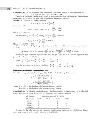
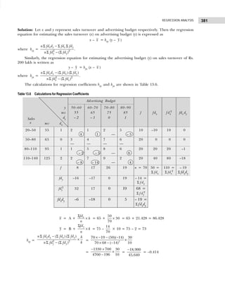
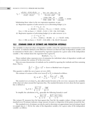
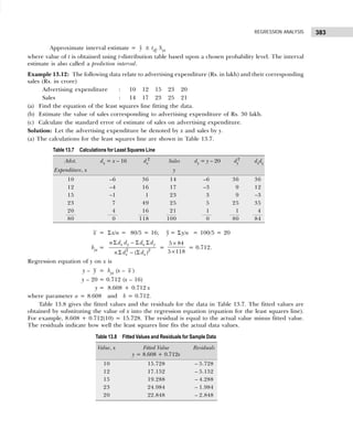
![BUSINESS STATISTICS: PROBLEMS AND SOLUTIONS
384
(b) The least squares equation obtained in part (a) may be used to estimate the sales turnover corresponding
to the advertising expenditure of Rs. 30 lakh as
ŷ = 8.608 + 0.712x = 8.608 + 0.712 (30) = Rs. 29.968 crore.
(c) Calculations for standard error of estimate Sy⋅x of sales (y) on advertising expenditure (x) are shown in
Table 13.9.
Sy⋅x =
2
2
y a y b xy
n
Σ − Σ − Σ
−
=
2080 8.608 100 0.712 1684
5 2
− × − ×
−
=
2080 860.8 1199
3
− −
= 2.594.
Example 13.13: The following table shows the ages (X) and blood pressure (Y) of 8 persons.
Age : 52 63 45 36 72 65 47 25
Blood Pressure : 62 53 51 25 79 43 60 33
Obtain the regression equation of y on x and find the expected blood pressure of person who is 49
years old. [Bombay Univ., B.Com., 1996]
Solution: Calculations for regression equation of blood pressure (y) on age (x) are shown below:
Age dx = (x – 50) dx
2
Blood Pressure (y) dy = (y – 50) dy
2
dx dy
52 20 4 62 12 144 24
63 13 169 53 +3 9 39
45 –5 25 51 +1 1 –5
36 –14 196 25 –25 625 350
72 22 484 79 29 841 638
65 15 225 43 –7 49 –105
47 –3 9 60 10 100 –30
25 –25 625 33 –17 289 425
405 5 1737 406 6 2058 1336
y =
406 405
= =50.75 and = = =50.625.
8 8
y x
x
n n
Σ Σ
The regression coefficient of y on x is given by
byx =
y
x
r
σ
σ
=
Σ − Σ Σ
Σ − Σ
2 2
( )
x y x y
x x
n d d d d
n d d
= 2
(8) (1336) (5) (6) 10688 30
= =0.768
13896 25
(8) (1736) (5)
− −
−
−
−
y y = ( )
y
x
r x x
−
σ
σ
Table 13.9 Calculations for Standard Error of Estimate
x y y2
xy
10 14 196 140
12 17 289 204
15 23 529 345
23 25 625 575
20 21 441 420
80 100 2080 1684](https://image.slidesharecdn.com/businessstatisticsproblemsandsolutions-230910073954-6d42a210/85/Business-Statistics_-Problems-and-Solutions-pdf-398-320.jpg)
![385
REGRESSION ANALYSIS
y – 50.75 = 0.768(x – 50.625)
y – 5.75 = 0.768 x – 38.88 or y = 11.87 + 0.765 x
Y49 = 11.87 + 0.768 (49) = 49.502 (When age of person is x = 49).
Thus, the expected blood pressure of a person who is 49 years old shall be 49.5.
Example 13.14: In a correlation study the following values are obtained:
X Y
Mean 65 67
Standard Deviation 2.5 3.5
Coefficient of Correlation, r = 0.8
Find the two regression equations that are associated with the above values.
[Kashmir Univ., B.Com., 1998; HP Univ., MBA, 2000]
Solution: Given that x =65, r = 0.8, σx = 2.5, σy = 3.5, y = 67.
Regression equation of y on x: x – x = ( ).
y
x
r y y
σ
σ
−
Substituting the values, x – 65 = −
2.5
8 ( )
3.5
y y = 0.5714 (Y – 67)
x – 65 = 0.5714 y – 38.25 or x = 26.72 + 0.5714 y.
Regression equation of y on x: y – y = −
( )
y
x
r x x
σ
σ
x – 67 = −
3.5
8 ( 65)
2.5
x = 11.2 (x – 65)
x – 67 = 11.2 x – 72.8 or y = –5.8 + 11.5x.
Example 13.15: For 50 students of a class the regression equation of marks in Statistics (x) on the marks
in Accountancy (y) is 3y – 5x + 180 = 0. The mean in Accountancy is 44 variance of marks in Statistics in
9/16th of the variance of marks in Accountancy. Find the mean marks in Statistics and the coefficient
between marks in the two subjects. [Delhi Univ., B.Com.(H), 2003; Jamia Milia Univ., M.Com., 2003, 2004]
Solution: The given regression equation is
3y – 5x + 180 = 0 or 3y + 180 = 5x,
where x represents marks in Statistics and y marks in Accountancy. When y = 44, x will be given by
5x = 3(44) + 180 = 0 or x = 312/5 = 62.4.
Hence, the mean marks in Statistics are 62.4.
Regression coefficient of x on y from the given equation is
5x = 3y + 180 or x = 0.6Y + 36
where bxy = 0.6;
y
x
r
σ
σ
=
9
16
=
3
4
(given).
Applying following formula for calculating coefficient of correlation,
bxy =
y
x
r
σ
σ
0.6 =
9
16
r or 0.6 =
3
4
r , i.e., r = 0.8.](https://image.slidesharecdn.com/businessstatisticsproblemsandsolutions-230910073954-6d42a210/85/Business-Statistics_-Problems-and-Solutions-pdf-399-320.jpg)
![BUSINESS STATISTICS: PROBLEMS AND SOLUTIONS
386
Example 13.16: You are given the following data:
X Y
Mean 65 67
Standard Deviation 2.5 3.5
Correlation coefficient between x and y = 0.66.
(a) Find the two regression equations.
(b) Estimate the value of x when y = 75. [Guwahati Univ., B.Com., 2005]
Solution: (a) Given that x = 36, r = 0.66, σx = 11, σy = 8, y = 85.
Regression equation of x on y: x – x = −
( )
y
x
r y y
σ
σ
x – 36 = −
11
0.66 ( 85)
8
y = 0.9075 (y – 85)
= 0.9075y – 77.1375 + 36 or x = –41.1375 + 0.9075y.
Regression equation of y on x: y – y = −
( )
y
x
r x x
σ
σ
y – 85 =
8
0.66 ( 36)
11
x − = 0.48(x – 36)
y – 85 = 0.48x – 17.28 or y = 67.72 + 0.48x.
(b) Using regression equation of x on y, to find the estimated value of x when y = 75
x = 0.9075 (75) – 41.1375 = 26.925.
Example 13.17: For certain x and y series which are correlated, the two lines of regression are
5x – 6y + 90 = 0 and 15x – 8y – 130 = 0.
Find the means of the two series and the correlation. [MD Univ., M.Com., 1998]
Solution: Solving two simultaneous regression equations to find mean value, we get x = 30 and y = 40.
Rewriting first regression equation as follows to find correlation coefficient, r,
6y = 5x + 90, i.e., y =
5
6
x + 15 or byx =
5
6
.
Also, 15x = 8y + 130, i.e., x =
8 130
15 15
y + or bxy =
8
15
.
Since both regression coefficients bxy and byx are less than one, applying following formula to get
correlation coefficient:
r =
8 5
= =0.667.
15 6
xy yx
b b
× ×
Example 13.18: From the following data obtain the two regression equations and calculate the correlation
coefficient:
X : 1 2 3 4 5 6 7 8 9
Y : 9 8 10 12 11 13 14 16 15
(a) Estimate the value of y which should correspond on an average to x = 6.2.
(b) Obtain correlation coefficient, r
[M.G. Univ., B.Com., 1997; Kumaon Univ., M.Com, 1998; Hyderabad Univ., MBA, 2005]](https://image.slidesharecdn.com/businessstatisticsproblemsandsolutions-230910073954-6d42a210/85/Business-Statistics_-Problems-and-Solutions-pdf-400-320.jpg)
![387
REGRESSION ANALYSIS
Solution: Required calculations for two regression equations and also for correlation coefficient are
shown in the table below:
Variable dx=(x – x ) dx
2
(y) dy = (y – y ) dy
2
dx dy
1 –4 16 9 –3 9 12
2 –3 9 8 –4 16 12
3 –2 4 10 –2 4 4
4 –1 1 12 0 0 0
5 0 0 11 –1 1 0
6 1 4 13 1 1 1
7 2 4 14 2 4 4
8 3 9 16 4 16 12
9 4 16 15 3 9 12
45 0 60 108 0 60 57
x =
Σ Σ
45 108
= = 5 and = = =12
9 9
x y
y
n n
.
Regression equation of x on y: x – x = −
( )
y
x
r y y
σ
σ
x – 5 = 0.95 (y – 12), where x
y
r
σ
σ
=
Σ
Σ 2
x y
y
d d
d
=
57
60
= 0.95
= 0.95y – 11.4 or x = –6.4 + 0.95y.
Regression equation of y on x: y – y = −
( )
y
x
r x x
σ
σ
y – 12 = 0.95(x – 5), where
y
x
r
σ
σ
=
Σ
Σ 2
57
= =0.95
60
x y
x
d d
d
= 0.95 x – 4.75 or y = 7.25 +0.95X.
Given x = 6.2, we get y = 0.95 (6.2) + 7.25 = 13.14.
(b) Substituting values of two regression coefficients byx and bxy in the following formula to get value of
correction coefficient.
r = ×
yx xy
b b = ×
0.95 0.95 = 0.95.
Example 13.19: Find the most likely production corresponding to a rainfall 40″ from the following
data:
Rainfall (x) Production (y)
Average 30″ 500 kg
Standard deviation 5″ 100 kg
Coefficient of correlation, r = 0.8 [Bhartidasan Univ., M.Com., 1996; GGSIP Univ., MBA, 2002]
Solution: Given that r = 0.8, x = 30, y = 500, σy = 100, and σx = 5.
The regression equation of production (y) on rainfall (x) is written as
y – y = −
( )
y
x
r x x
σ
σ
y – 500 = −
100
8 ( 30)
5
x = 16x – 480 or y = 20 + 16x.
When rainfall x = 40″, the likely production will be y = 16(40) + 20 = 660 kg.](https://image.slidesharecdn.com/businessstatisticsproblemsandsolutions-230910073954-6d42a210/85/Business-Statistics_-Problems-and-Solutions-pdf-401-320.jpg)
![BUSINESS STATISTICS: PROBLEMS AND SOLUTIONS
388
Example 13.20: The following data, based on 450 students, are given for marks is Statistics and Economics
at a certain examination:
Mean marks in Statistics : 40
Mean marks in Economics : 48
S.D. of marks in Statistics : 12
The variance of marks in Economics : 256
Sum of the product of deviation of marks from their respective mean : 42075
Obtain equations of the two lines of regression and estimate the average marks in Economics of
candidates who obtained 50 marks in Statistics. [Nagpur Univ., M.Com., 1996]
Solution: Let the marks in Statistics be denoted by x and marks in Economics by y. Then given that
x = 40, y = 48, σx = 12, σy = 256 = 16.
Regression equation of x on y: x – x = −
( )
x
y
r y y
σ
σ
x – 40 = −
12
0.487 ( 48)
16
y , where r =
42075
= = 0.487
450 12 16
x y
x y
d d
n
Σ
× ×
σ σ
= 0.365 y – 17.52 or x = 22.48 + 0.365y.
Regression equation of y on x: y – y = −
( )
y
x
r x x
σ
σ
y – 48 = 0 −
16
.487 ( 40)
12
x
= 0.649x – 25.96 or y = 22.04 + 0.649x.
The estimated marks in Economics for a candidate who has obtained x = 50 marks in Statistics will be
y = 22.04 + 0.649 (50) = 54.49.
Example 13.21: Two random variables have the regression equations
3x – 2y – 26 = 0 and 6x – y – 31 = 0.
Find the mean value and the coefficient of correlation between x and y. If the variance of σx
2
= 25,
find the standard deviation of y from the data given above.
[MD Univ., B.Com.(H), 2004; MDS Univ., M.Com., 2004; Delhi Univ., B.Com.(H), 2005]
Solution: Solving simultaneous regression equations for x and y we get x = 4 and y = 7.
To find coefficient of correlation, determine the value of regression coefficients from the two regression
equations as follows:
Rewritting first regression equation as
2y = 26 – 3x or y =
−
−
3 3
13 or =
2 2
yx
x b .
Also, rewritting second regression equation as
6x = 31 – y or x =
−
−
31 1 1
or =
6 6 6
xy
y b .
Thus, correlation coefficient, r =
3 1
= = 0.5
2 6
xy yx
b b
× − × − .
To find standard deviation in y series, applying the following formula,
bxy =
y
x
r
σ
σ
3
2
−
= 0.5
5
y
−
σ
, i.e., 5(–1.5) = –0.5σy or σy = 15.](https://image.slidesharecdn.com/businessstatisticsproblemsandsolutions-230910073954-6d42a210/85/Business-Statistics_-Problems-and-Solutions-pdf-402-320.jpg)
![389
REGRESSION ANALYSIS
Example 13.22: The following table gives the aptitude test scores and productivity indices of 10 workers
selected at random:
Aptitude scores (x) : 60 62 65 70 72 45 53 73 65 82
Productivity index (y) : 68 60 62 80 85 40 52 62 60 81
Calculate the two regression equations and estimate (a) the productivity index of a worker whose test
score is 92 and (b) the test score of a worker whose productivity index is 75.
[Delhi Univ., MBA, 1998; GGSIP Univ., MBA, 2003; Hyderabad Univ., MBA, 2004]
Solution: Required calculations for two regression equations are shown in the table below:
Aptitude dx = x – 65 dx
2
Productivity dy = y – 65 dy
2
dx dy
Score (x) Index (y)
60 –5 25 68 3 9 –15
62 –3 9 60 –5 25 15
65 0 0 62 –3 9 0
70 5 25 80 15 225 75
72 7 49 85 20 400 140
48 –17 289 40 –25 625 425
53 –12 144 52 –13 169 156
73 8 64 62 –3 9 –24
65 0 0 60 –5 25 0
82 17 289 81 16 256 272
650 0 894 650 0 1752 1044
x =
650 650
= = 65 and = = = 65
10 10
x y
y
n n
Σ Σ
dxy = x
y
r
σ
σ
= 2
1044
= =0.596
1752
x y
y
d d
d
Σ
.
Regression equation of x on y: x – x = ( )
x
y
r Y Y
σ
σ
−
x – 65 = 0.596(y – 65)
= 0.596y – 38.74 or x = 26.26 + 0.596y.
When y = 75, the corresponding value of x becomes
x = 26.26 + 0.596 (75) = 70.96.
Thus, the aptitude score of a worker is 70.96 whose productivity index is 75.
Regression equation of y on x: y – y = −
( )
y
x
r x x
σ
σ
y – 65 = 1.168(x – 65), where dyx =
Σ
Σ 2
1044
= =1.168
894
x y
x
d d
d
= 1.168x – 75.92 or y = –10.92 +1.168x.
When x = 92, the corresponding value of y becomes y92 = –10.92 + 1.168(92) = 96.536. Thus, the
productivity index of a worker is 96.536 whose score is 92 points.
Example 13.23: From 10 observations of price (m) and supply (n) of a commodity, the following summary
figures were obtained (in appropriate units):
Σ m = 130; Σ n = 220; Σ m2
= 2288; Σ n2
= 5506; and Σ mn = 3467
Compute a regression line of n on m and estimate the supply when the price is 16.](https://image.slidesharecdn.com/businessstatisticsproblemsandsolutions-230910073954-6d42a210/85/Business-Statistics_-Problems-and-Solutions-pdf-403-320.jpg)
![BUSINESS STATISTICS: PROBLEMS AND SOLUTIONS
390
Solution: Given that n =
Σ 220
= = 22
10
n
n
and
130
= = =13.
10
m
m
n
∑
Regression line of n on m is given by
n – n = ( )
n
m
r m m
σ
σ
− , where n
m
r
σ
σ
=
( )2
2
n mn n m
n m m
− ×
∑ ∑ ∑
−
∑ ∑
=
607
=1.015.
598
n – 22 = 1.015 (m – 13)
= 1.015 m – 13.195
n = 1.015 m + 8.805.
When price m = 16, the corresponding supply n becomes
n = 1.015 (16) + 8.805 = 25.045.
Thus, the estimated supply is of 25.45 units when price is 16 units.
Example 13.24: For a given set of bivariate data, the following results were obtained.
x = 53.2, y = 27.9, Regression Coefficient of y on x = –1.5.
Regression coefficient of x on y = –0.2. Find the most probable value of y when x is 60.
[Mysore Univ., B.Com., 1999]
Solution: For finding the most probable value of y when x = 60, a regression equation of y on x is:
y – y = ( )
y
x
r x x
−
σ
σ
, where y = 27.9, r = = 1.5, and =53.2.
y
x
r x
−
σ
σ
y – 27.9 = 1.5(x – 53.2)
= –1.5 x + 79.8 or y = 107.7 – 1.5 x.
For x = 60, y = 107.7 – 1.5 (60) = 17.7 and r = = 0.2 1.5 = 0.548
xy yx
b b
× − × − − .
Example 13.25: You are given the following information about advertising expenditure and sales:
Adv. Exp. (x) Sales (x)
(Rs. crore) (Rs. crore)
Mean 20 120
Standard deviation 5 25
Correlation coefficient is 0.8.
(a) Calculate two regression lines.
(b) Find the likely sales when advertisement expenditure is Rs. 25 crore.
(c) What should be the advertisement budget if the company wants to attain sales target of Rs. 150 crore?
[Jammu Univ., M.Com., 2004]
Solution: Given: x = 20, y = 120, σx = 5, σy = 25, and r = 0.8.
(a) Regression equation of x on y: x – x = −
( )
x
y
r y y
σ
σ
x – 20 = −
5
0.8 ( 120)
25
y = 0.16(y – 120)
= 0.16y – 19.2 or x = 0.8 + 0.16y.
Regression equation of y on x: y – y = −
( )
y
x
r x x
σ
σ
y – 120 = −
25
0.8 ( 20)
5
x = 4(x – 20)
y – 120 = 4x – 80 or y = 40 + 4x.](https://image.slidesharecdn.com/businessstatisticsproblemsandsolutions-230910073954-6d42a210/85/Business-Statistics_-Problems-and-Solutions-pdf-404-320.jpg)
![391
REGRESSION ANALYSIS
(b) Using regression equation of y on x, to find the likely sales when advertisement expenditure is
Rs. 25 crore, that is, y25 = 4 (25) + 40 = Rs. 140 crore. Hence, the likely sales when advertisement
expenditure is Rs. 25 crore is Rs. 140 crore.
(c) Using regression equation of x on y, to find the advertisement budget when sales target is of Rs. 150
crore, that is, x150 = 0.016 (150) + 0.8 = 24 + 0.8 = Rs. 24.8 crore
Hence, to attain a sales target of Rs. 150 crore, the advertisement budget must be Rs. 24.8 crore.
S e l f-P r a c t i c e P r o b l e m s 13A
13.1 The following calculations have been made for prices
of twelve stocks (x) at the Calcutta Stock Exchange on
a certain day along with the volume of sales in
thousands of shares (y). From these calculations find
the regression equation of price of stocks on the
volume of sales of shares.
Σ x = 580, Σy = 370, Σxy = 11494,
Σ x2
= 41658, Σy2
= 17206.
[Rajasthan Univ., M.Com., 1995]
13.2 A survey was conducted to study the relationship
between expenditure (in Rs.) on accommodation (x)
and expenditure on food and entertainment (y) and
the following results were obtained:
Mean Standard
Deviation
Expenditure on 173..1 63.15
accommodation
Expenditure on food 47.8 22.98
and entertainment
Coefficient of correlation, r = 0.57
Write down the regression equation and estimate the
expenditure on food and entertainment if the
expenditure on accommodation is Rs. 200.
[Bangalore Univ., B.Com., 1998]
13.3 The following data give the experience of machine
operators and their performance ratings given by the
number of good parts turned out per 100 pieces:
Operator : 11 12 13 4 5 16 7 18
experience (x) : 16 12 18 4 3 10 5 12
Performance
ratings (y) : 87 88 89 68 78 80 75 83
Calculate the regression lines of performance ratings
on experience and estimate the probable performance
if an operator has 7 years experience.
[Jammu Univ., M.Com.; Lucknow Univ., MBA, 1996]
13.4 A study of prices of a certain commodity at Delhi and
Mumbai yield the following data:
Delhi Mumbai
Average price per kilo (Rs.) 2.463 2.797
Standard deviation 0.326 0.207
Correlation coefficient
between prices at Delhi
and Mumbai, r = 0.774
Estimate from the above data the most likely price (a)
at Delhi corresponding to the price of Rs. 2.334 per
kilo at Mumbai and (b) at Mumbai corresponding to
the price of 3.052 per kilo at Delhi.
13.5 The following table gives the aptitude test scores and
productivity indices of 10 workers selected at random:
Aptitude
scores (x): 60 62 65 70 72 48 53 73 65 82
Productivity
index (y): 68 60 62 80 85 40 52 62 60 81
Calculate the two regression equations and estimate
(a) the productivity index of a worker whose test score
is 92 and (b) the test score of a worker whose
productivity index is 75. [Delhi Univ., MBA, 2001]
13.6 A company wants to assess the impact of R&D
expenditure (Rs. in 1000s) on its annual profit (Rs. in
1000’s). The following table presents the information
for the last eight years:
Year R & D Expenditure Annual Profit
1991 9 45
1992 7 42
1993 5 41
1994 10 60
1995 4 30
1996 5 34
1997 3 25
1998 2 20](https://image.slidesharecdn.com/businessstatisticsproblemsandsolutions-230910073954-6d42a210/85/Business-Statistics_-Problems-and-Solutions-pdf-405-320.jpg)
![BUSINESS STATISTICS: PROBLEMS AND SOLUTIONS
392
Estimate the regression equation and predict the
annual profit for the year 2002 for an allocated sum
of Rs. 1,00,000 as R&D expenditure.
[ Jodhpur Univ., MBA, 1998]
13.7 Obtain the two regression equations from the following
bivariate frequency distribution:
Sales Revenue Advertising Expenditure (Rs. in thousand)
(Rs. in lakh) 5–15 15–25 25–35 35–45
75–125 3 4 4 8
125–175 8 6 5 7
175–225 2 2 3 4
225–275 3 3 2 2
Estimate (a) the sales corresponding to advertising
expenditure of Rs. 50,000, (b) the advertising
expenditure for a sales revenue of Rs. 300 lakh, and (c)
the coefficient of correlation. [Delhi Univ., MBA, 2002]
13.8 The personnel manager of an electronic
manufacturing company devises a manual test for job
applicants to predict their production rating in the
assembly department. In order to do this he selects a
random sample of 10 applicants. They are given the
test and later assigned a production rating. The results
are as follows:
Worker : A B C D E F G H I J
Test score : 53 36 88 84 86 64 45 48 39 69
Production
rating : 45 43 89 79 84 66 49 48 43 76
Fit a linear least squares regression equation of
production rating on test score.
[Delhi Univ., MBA, 2002]
13.9 Find the regression equation showing the capacity
utilization on production from the following data:
Average Standard
Deviation Deviation
Production 35.6 10.5
(in lakh units) :
Capacity utilization
(in percentage) : 84.8 8.5
Correlation coefficient r = 0.62
Estimate the production when the capacity utilization
is 70 per cent.
[Delhi Univ., MBA, 1997; Pune Univ., MBA, 1998]
13.10 Suppose that you are interested in using past
expenditure on R&D by a firm to predict current
expenditures on R&D. You got the following data by
taking a random sample of firms, where x is the amount
spent on R&D (in lakh of rupees) 5 years ago and y is
the amount spent on R&D (in lakh of rupees) in the
current year:
x : 30 50 20 180 10 20 20 40
y : 50 80 30 110 20 20 40 50
(a) Find the regression equation of y on x.
(b) If a firm is chosen randomly and x = 10, can you
use the regression to predict the value of y? Discuss.
[Madurai-Kamraj Univ., MBA, 2000]
13.11 The following data relate to the scores obtained by
the salesmen of a company in an intelligence test and
their weekly sales (in Rs. 1000’s ):
Salesman
intelligence : A B C D E F G H I
Test score : 50 60 50 60 80 50 80 40 70
Weekly sales : 30 60 40 50 60 30 70 50 60
(a) Obtain the regression equation of sales on intelli-
gence test scores of the salesmen.
(b) If the intelligence test score of a salesman is 65,
what would be his expected weekly sales?
[HP Univ., M.Com., 1996]
13.12 Two random variables have the regression equations:
3x + 2y – 26 = 0 and 6x + y – 31 = 0
(a) Find the mean values of x and y and coefficient of
correlation between x and y.
(b) If the varaince of x is 25, then find the standard
deviation of y from the data.
[MD Univ., M.Com., 1997; Kumaon Univ., MBA, 2001]
13.13 For a given set of bivariate data, the fiollowing results
were obtained
x = 53.2, y = 27.9,
Regression coefficient of y on x = – 1.5 and Regres-
sion coefficient of x and y = – 0.2.
Find the most probable value of y when x = 60.
13.14 In trying to evaluate the effectiveness in its advertising
compaign, a firm compiled the following information:
Calculate the regression equation of sales on advertis-
ing expenditure. Estimate the probable sales when
advertisement expenditure is Rs. 60,000.
Year Advt. Expenditure Sales
(Rs. 1000’s) (in lakhs Rs.)
1996 12 5.0
1997 15 5.6
1998 17 5.8
1999 23 7.0
2000 24 7.2
2001 38 8.8
2002 42 9.2
2003 48 9.5
[Bharathidasan Univ., MBA, 2003]](https://image.slidesharecdn.com/businessstatisticsproblemsandsolutions-230910073954-6d42a210/85/Business-Statistics_-Problems-and-Solutions-pdf-406-320.jpg)
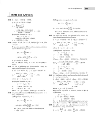
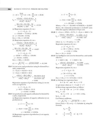
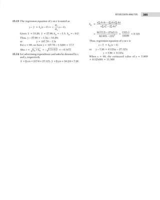
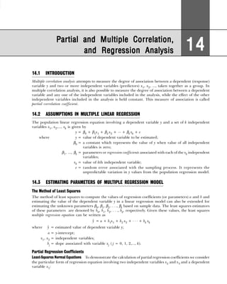
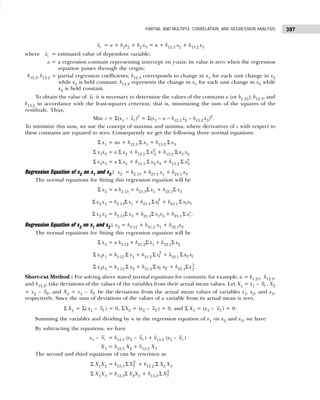
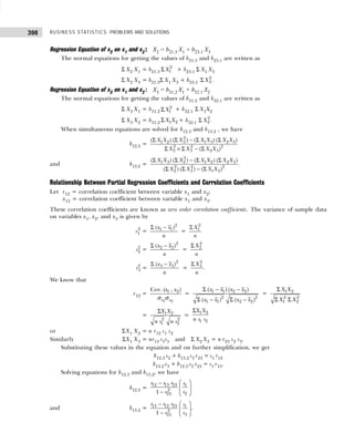
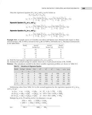
![BUSINESS STATISTICS: PROBLEMS AND SOLUTIONS
400
Multiply Eq. (i) by 21 and Eq. (iii) by 5 to eliminate a, we get
777 = + 105a + 1533b1 + 441b2
+ 720 = + 105a + 1495b1 + 475b2
– 720 = – – – 4375b2
(v) 57 = + 105a + 1438b1 – 4334b2
Multiplying Eq. (iv) by 34 and Eq. (v) by 38 to eliminate b2, we get
6596 = +11764b1 – 1292b2
+ 1406 = + 1444b1 – 1292b2
– 1406 = – 1444b1 + 1292b2
5190 = 10320b1 or b1 = 0.502
Substituting the value of b1 in Eqn. (i) and (ii), we get
(vi) 5a + 21b2 = – 0.354
(vii) 21a + 95b2 = – 6.098
Multiplying Eq. (vi) by 21 and Eq. (vii) by 5 to eliminate a, we get
105a + 441b2 = – 7.434
+ 105a + 475b2 = – 30.49
– – 475b2 = +30.49
– 34b2 = 37.924 or b2 = –1.115
Substituting the value of b1 and b2 in Eqn. (i), we get a = 4.753.
(a) The least-squares regression equation of x1 on x2 and x3 is given by
x1 = a + b1x2 + b2 x3 = 4.753 + 0.502 x2 – 1.115 x3.
(b) The estimated value of annual savings (x1) is obtained by substituting annual income x2 = Rs. 1600
and family size x3 = 4, as
1
x̂ = 4.753 + 0.502(1600) – 1.115(4) = Rs. 803.493.
Example 14.2: An instructor of mathematics wishes to determine the relationship of grades in the final
examination to grades on two quizes given during the semester. Let x1, x2, and x3 be the grades of a
student in the first quiz, second quiz, and final examination, respectively. The instructor made the
following computations for a total of 120 students:
1
x = 6.80 2
x = 0.70 3
x = 74.00
s1 = 1.00 s2 = 0.80 s3 = 9.00
r12 = 0.60 r13 = 0.70 r23 = 0.65
(a) Find the least-squares regression equation of x3 on x1 and x2.
(b) Estimate the final grades of two students who scored respectively 9 and 7 and 4 and 8 marks in the
two quizes. [HP Univ., MBA, 1998]
Solution: (a) The regression equation of x3 on x2 and x1 can be written as
(x3 – 3
x ) = ( ) ( )
23 13 12 13 23 12
3 3
2 2 1 1
2 2
2 1
12 12
1 1
r r r r r r
s s
x x x x
s s
r r
− −
− + −
− −
.
Substituting the given values, we have
(x3 – 74) =
0.65 0.7 0.6 9
1 (0.6)2 0.8
− ×
−
(x2 – 7) + 2
0.7 0.65 0.6 9
1
1 (0.6)
− ×
−
(x1 – 6.8)
(x3 – 74) = 2 1
0.65 0.42 0.7 0.39
9
( 7) (9) ( 6.8)
0.64 0.8 0.64
x x
− −
− + −
](https://image.slidesharecdn.com/businessstatisticsproblemsandsolutions-230910073954-6d42a210/85/Business-Statistics_-Problems-and-Solutions-pdf-414-320.jpg)
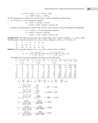
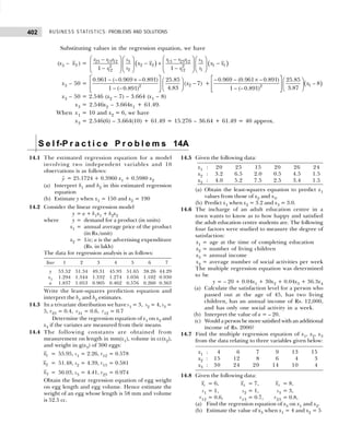
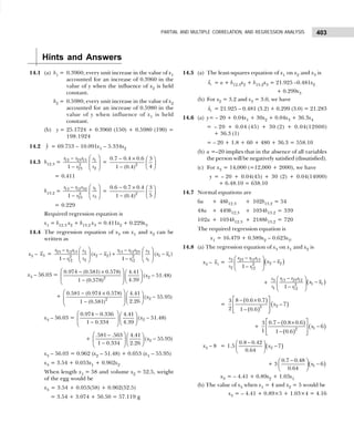
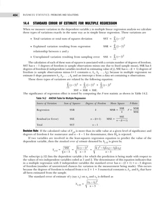
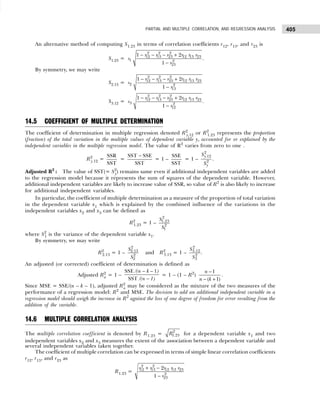
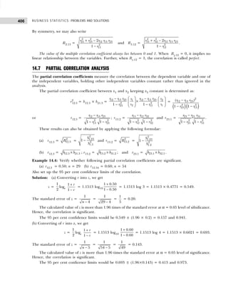
![407
PARTIAL AND MULTIPLE CORRELATION, AND REGRESSION ANALYSIS
Relationship Between Multiple and Partial Correlation Coefficients
The results connecting multiple and partial correlation coefficients are as follows:
• 1 – R2
1.23 = (1 – r2
12) (1 – r2
13.2),
1 – R2
2.13 = (1 – r2
21) (1 – r2
23.1),
1 – R2
3.12 = (1 – r2
31) (1 – r2
32.1).
• 1 – R1.234 = (1 – r2
12) (1 – r2
13.2) (1 – r2
14.23).
Example 14.5: The correlation between a general intelligence test and school achievement in a group of
children aged 6 to 15 years is 0.80. The correlation between the general intelligence test and age in the
same group is 0.70 and the correlation between school achievement and age is 0.60. What is the correlation
between general intelligence and school achievement in children of the same age? Comment on the
result.
Solution: Let x1 = general intelligence test; x2 = school achievement; x3 = age of children.
Given r12 = 0.8, r13 = 0.7, and r23 = 0.6. Then the correlation between general intelligence test and
school achievement, keeping the influence of age as constant, we have
r12.3 = 12 13 23
2 2
13 23
1 1
r r r
r r
−
− −
=
2 2
0.8 0.7 0.6
1 (0.7) 1 (0.6)
− ×
− −
=
0.8 0.42
0.51 0.64
−
=
0.38
0.57
= 0.667.
Hence, we conclude that intelligence and school achievement are associated to each other to the
extent of r12.3 = 0.667 while the influence of the children’s age is held constant.
Example 14.6: In a trivariate distribution it is found that r12 = 0.70, r13 = 0.61, and r23 = 0.40. Find the
values of r23.1, r13.2, and r12.3. [Delhi Univ., M.Com., 1998]
Solution: The partial correlation between variables 2 and 3 keeping the influence of variable 1 constant
is given by
r23.1 = 23 12 13
2 2
12 13
1 1
r r r
r r
−
− −
.
Substituting the given values, we get
r23.1 =
2 2
0.40 0.70 0.61
1 (0.70) 1 (0.61)
− ×
− −
=
0.40 0.427
0.51 0.6279
−
=
0.027
0.714 0.7924
×
=
0.027
0.5657
= 0.0477.
Similarly, we get r13.2 =
− ×
− −
13 12 23
2 2
12 23
1 1
r r r
r r
=
2 2
0.61 0.70 0.40
1 (0.70) 1 (0.40)
− ×
− −
= 0.504
r12.3 =
− ×
− −
12 13 23
2 2
13 23
1 1
r r r
r r
=
2 2
0.70 0.61 0.40
1 (0.61) 1 (0.40)
− ×
− −
= 0.633.
Example 14.7: Based on the following data, calculate R1.23, R3.12, and R2.13.
[HP Univ., MBA, 1997]
Solution: The coefficient of multiple determination of two independent variables coded as 2 and 3 is
given by
1
x = 6.8 2
x = 7.0 3
x = 74
s1 = 1.0 s2 = 0.8 s3 = 9
r12 = 0.6 r13 = 0.7 r23 = 0.65](https://image.slidesharecdn.com/businessstatisticsproblemsandsolutions-230910073954-6d42a210/85/Business-Statistics_-Problems-and-Solutions-pdf-421-320.jpg)
![BUSINESS STATISTICS: PROBLEMS AND SOLUTIONS
408
R1.23 =
2 2
12 13 12 13 23
2
23
2
1
r r r r r
r
+ −
−
.
Substituting the given values, we get
R1.23 =
2 2
2
(0.6) (0.7) 2 0.6 0.7 0.65
1 (0.65)
+ − × × ×
−
=
0.36 0.49 0.546
0.5775
+ −
= 0.526 = 0.725.
Similarly,
R3.12 =
2 2
31 23 12 13 23
2
12
2
1
r r r r r
r
+ −
−
=
2 2
2
(0.7) (0.65) 2 0.6 0.7 0.65
1 (0.6)
+ − × × ×
−
=
0.49 0.4225 0.546
1 0.36
+ −
−
= 0.573 = 0.757
R2.13 =
2 2
12 23 12 13 23
2
13
2
1
r r r r r
r
+ −
−
=
2 2
2
(0.6) (0.65) 2 0.6 0.7 0.65
1 (0.7)
+ − × × ×
−
=
0.36 0.4225 0.546
0.51
+ −
= 0.464 = 0.681.
Example 14.8: Suppose a computer has found, for a given set of values of variables x1, x2, and x3, the
correlation coefficients are r12 = 0.91, r13 = 0.33, and r23 = 0.81. Explain whether these computations
may be said to be free from errors. [Madurai Kamaraj Univ., B.Com., 1989]
Solution: For determining whether the given computations are correct or not, we calculate the value of
the partial correlation coefficient r12.3 for variables 1 and 2 keeping the influence of variable 3 constant.
If the value of r12.3 is less than one, then the computations may be said to be free from errors.
r12.3 = 12 13 23
2 2
13 23
1 1
r r r
r r
−
− −
=
2 2
0.91 (0.33) (0.81)
1 (0.33) 1 (0.81)
−
− −
=
0.91 0.2673
1 0.1089 1 0.6561
−
− −
=
0.6427
0.8911 0.3439
×
= 1.161.
Since the calculated values of r12.3 is more than one, the computations given in the question are not
free from errors.
Example 14.9: The simple correlation coefficients between temperature (x1), yield of corn (x2), and
rainfall (x3) are r12 = 0.59, r13 = 0.46, and r23 = 0.77. Calculate the partial correlation coefficient r12.3 and
multiple correlation coefficient R1.23. [Delhi Univ., M.Com.; HP Univ., MBA, 1996]
Solution: Partial correlation coefficient r12.3 is defined as
r12.3 = 12 13 23
2 2
13 23
1 1
r r r
r r
−
− −
.
Substituting the given values, we get
r12.3 =
2 2
0.59 0.46 0.77
1 (0.46) 1 (0.77)
− ×
− −
=
0.59 0.3542
1 0.2116 1 0.5529
−
− −
=
0.2358
0.5665
= 0.416.
Multiple correlation coefficient is defined as
R1.32 =
2 2
12 13 12 13 23
2
23
2
1
r r r r r
r
+ −
−
=
2 2
2
(0.59) (0.46) 2 (0.59 0.46 0.77)
1 (0.77)
+ − × ×
−
=
0.3481 0.2116 0.418
0.4071
+ −
=
0.5597 0.418
0.4071
−
=
0.1417
0.4071
= 0.589.](https://image.slidesharecdn.com/businessstatisticsproblemsandsolutions-230910073954-6d42a210/85/Business-Statistics_-Problems-and-Solutions-pdf-422-320.jpg)

![BUSINESS STATISTICS: PROBLEMS AND SOLUTIONS
410
Example 14.12: The following values have been obtained from the measurement of three variables x1, x2,
and x3.
1
x = 6.80 2
x = 7.00 3
x = 7.40
s1 = 1.00 s2 = 0.80 s3 = 0.90
r12 = 0.60 r13 = 0.70 r23 = 0.65
(a) Obtain the regression equation of x1 on x2 and x3
(b) Estimate the value of x1 for x2 = 10 and x2 = 9
(c) Find the coefficient of multiple determination R2
1.23 from r12 and r13.2
Solution: (a) The regression equation of x1 on x2 and x3 is given by
(x1 – 1
x ) = 12 13 23 13 12 23
1 1
2 2 3 3
2 2
2 3
23 23
( ) ( )
1 1
r r r r r r
s s
x x x x
s s
r r
− −
− + −
− −
x1 – 6.8 = 2
2
0.60 0.70 0.65 1
( 7)
0.80
1 (0.65)
x
− ×
−
−
+ ( )
3
2
0.70 0.60 0.65 1
7.4
0.90
1 10.657
x
− ×
−
−
x1 – 6.8 = 2
0.60 0.455
(1.25) ( 7)
0.578
x
−
−
+ 3
0.70 0.39
(1.111) ( 7.4)
0.578
x
−
−
= 0.181 (x2 – 7) + 0.595 (x3 – 7.4)
or x1 = 5.670 + 0.181x2 + 0.595x3.
(b) Substituting x2 = 10 and x2 = 9 in the regression equation obtained in part (a), we have
x1 = 5.670 + 0.181(10) + 0.595 (9) = 12.835.
(c) Multiple and partial correlation coefficients are related as
R2
1.23 = 1 – (1 – r2
12) (1 – r2
13.2)
r13.2 = 13 12 23
2 2
12 23
1 1
r r r
r r
−
− −
=
2 2
0.70 0.60 0.65
1 (0.60) 1 (0.65)
− ×
− −
=
0.70 0.39
0.8 0.760
−
×
= 0.509
or r2
13.2 = 0.259.
Substituting values for r2
12 and r2
13.2 for R2
1.23, we have
R2
1.23 = 1 – (1 – 0.36) (1 – 0.259) = 0.526.
14.8 MISCELLANEOUS SOLVED EXAMPLES
Example 14.13: Find the multiple linear regression equation of x1 on x2 and x3 from the data relating to
three variables given below:
x1 : 4 6 7 9 13 15
x2 : 15 12 8 6 4 3
x3 : 20 24 20 14 10 4
[S.V
. Univ., MBA, 2002; Delhi Univ., M.Com., 2004]
Solution: The regression equation of x1 on x2 and x3 is
x1 = a1.23 + b12.3 x2 + b13.2 x3.
The value of the constants a1.23, b12.3, and b13.2 are obtained by solving the following three normal equations:
Σ x1 = na1.23 + b12.3 Σ x2 + b13.2 Σ x3
Σ x1 x2 = a1.23 Σ x2 + b12.3 Σ x2
2 + b13.2 Σ x2 x3
Σ x1 x3 = a1.23 Σ x3 + b12.3 Σ x2 x3 + b13.2 Σ x2
3.](https://image.slidesharecdn.com/businessstatisticsproblemsandsolutions-230910073954-6d42a210/85/Business-Statistics_-Problems-and-Solutions-pdf-424-320.jpg)
![411
PARTIAL AND MULTIPLE CORRELATION, AND REGRESSION ANALYSIS
Other calculations for the required values are shown below:
x1 x2 x3 x1 x2 x1 x3 x2 x3 x2
2
x2
3 x2
1
4 15 30 60 120 450 225 900 16
6 12 24 72 144 288 144 576 36
7 8 20 56 140 160 64 400 49
9 6 14 54 125 84 36 196 81
13 4 10 52 130 40 16 100 169
15 3 4 45 60 12 9 16 225
54 48 102 339 720 1,034 494 2,188 576
Subsitituting the values in the normal equations :
6 a1.23 + 48 b12.3 + 102 b13.2 = 54 (i)
48 a1.23 + 494 b12.3 + 1034 b13.2 = 339 (ii)
102 a1.23 + 1034 b12.3 + 2188 b13.2 = 720 (iii)
Multiplying Eq. (i) by 8, we get
48 a1.23 + 384 b12.3 + 816 b13.2 = 432 (iv)
Subtracting Eq. (ii) from Eqn. (iv), we get
110 b12.3 + 218 b13.2 = 93 (v)
Multiplying Eq. (i) by 17, we get
102 a1.23 + 816 b12.3 + 1734 b13.2 = 918 (vi)
Subtracting Eq. (vi) from Eq. (iii), we get
218 b12.3 + 454 b13.2 = – 198 (vii)
Multiplying Eq. (v) by 218, we get
23980 b12.3 + 47524 b13.2 = 20274 (viii)
Also multipling Eq. (vii) by 110, we get
23980 b12.3 + 49940 b13.2 = –21780 (ix)
Subtracting Eqn (viii) from Eqn (ix), we get
2416 b13.2 = –4205 or b13.2 = –17.40
Substituting the value of b13.2 in Eq. (v), we get
110 b12.3 = –218(–17.40) + 93 or b12.3 = 34.48
Subsituting the values of b12.3 and b13.2 in Eq. (i), we get
6 a1.23 + 48 (34.48) + 102 (–17.40) = 54
6 a12.3 + 1655.04 – 1774.80 = 54
6 a12.3 = 173.76 or a13.3 = 28.96.
Thus, the required regression equation is
x1 = 28.96 + 34.48 x2 – 17.40 x3.
Example 14.14: Given the following, determine the regression equation of
(a) x1 on x2 and x3
(b) x2 on x1 and x3
r12 = 0.8; r13 = 0.6; r23 = 0.5;
σ1 = 10; σ2 = 8; σ3 = 10. [Punjab Univ., M.Com., 2006]
Solution: (a) Regression equations of x1 on x2 and x3 is given by
x1 = b12.3 x2 + b13.2 x3
where b12.3 = 12 13 23
1
2
2 23
1
r r r
r
−
×
−
σ
σ
= 2
0.8 (0.6) (0.5)
10
= 0.833
8 1 (0.5)
−
×
−
;](https://image.slidesharecdn.com/businessstatisticsproblemsandsolutions-230910073954-6d42a210/85/Business-Statistics_-Problems-and-Solutions-pdf-425-320.jpg)
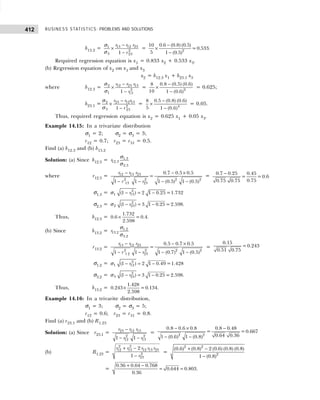
![413
PARTIAL AND MULTIPLE CORRELATION, AND REGRESSION ANALYSIS
Example 14.17: The correlation between a general intelligence test and school achievement in a group
of children from 6 to 15 years old is 0.80. The correlation between the general intellegence test and age
in the same group is 0.70 and the correlation between general intelligence and school achievement in
children of the same age is 0.6. Comment on the result.
Solution: Let x1 = general intelligence test
x2 = school achievement
x3 = age.
Given that r12 = 0.8, r13 = 0.7, and r23 = 0.6. Thus,
r12.3 =
−
− −
12 13 23
2 2
13 23
1 1
r r r
r r
=
2 2
0.8 0.7 0.6
1 (0.7) 1 (0.6)
− ×
− −
=
0.8 0.42 0.38
= =0.667.
0.57
0.51 0.64
−
Example 14.18: An instructor of mathematics wishes to determine the relationship of grades on a final
examination to grades on two quizes given during the semester. Costing x1, x2, and x3 the grades of a
student on the first quiz, second quiz, and final examination, respecttively, he made the following
computations for a total of 120 students:
1
x = 6.8; 2
x = 0.7; 3
x = 74;
s1 = 1.0; s2 = 0.80; s3 = 9.0;
r12 = 0.60; r13 = 0.70; r23 = 0.65.
(a) Find the least square regression equation of x3 on x1 and x2.
(b) Estimate the final grades to two students who scored, resepectively, 9 and 7, 4 and 5 in the two quizes.
[HP Univ., MBA, 1998]
Solution: (a) The regression equation of x3 on x1 and x2.
−
3 3
( )
x x =
− −
− + −
− −
23 12 13 13 23 12
3 3
2 2 1 1
2 2
2 1
12 12
( ) ( )
1 1
r r r r r r
s x
x x x x
s s
r r
(x3 – 74) =
− × − ×
− + −
− −
2 1
2 2
0.65 0.7 0.6 0.7 0.65 0.6
9 9
( 7) ( 6.8)
0.8 1
1 (0.6) 1 (0.6)
x x
=
− −
− + −
2 1
0.65 0.42 0.7 0.39
9
( 7) (9) ( 6.8)
0.64 0.8 0.64
x x
= 4.04 (x2 – 7) + 4.36 (x1 – 6.8)
= 4.04 x2 – 28.28 + 4.36 x1 – 29.65
x3 = 16.07 + 4.36 x1 + 4.04 x2.
(b) Final grades of students who scored x1 = 9 and x2 = 7 marks are
x3 = 16.07 + 4.36 (9) + 4.04 (7) = 83.59 or 84.
Final grades of students who scored x1 = 4 and x2 = 5 marks are
x2 = 16.04 + 4.36 (4) + 4.04 (5) = 53.68 or 54.
Example 14.19: Calculate (a) R1.23, (b) R3.12, and (c) R2.13 for the following data:
1
x = 6.8; 2
x = 7.0; 3
x = 74;
s1 = 1.0; s2 = 0.8; s3 = 9;
r12 = 0.6; r13 = 0.7; r23 = 0.65. [HP
, Univ., MBA, 2005]
Solution: (a) R1.23 =
+ −
−
2 2
12 13 12 13 23
2
23
2
1
r r r r r
r
=
+ − × × ×
−
2 2
2
(0.6) (0.7) 2 0.6 0.7 0.65
1 (0.65)
=
0.36 0.49 0.546
= 0.526 =0.725.
0.5776
+ −
R3.12 =
+ −
−
2 2
13 23 12 13 23
2
12
2
1
r r r r r
r
=
+ − × × ×
−
2 2
2
(0.7) (0.65) 2 0.6 0.7 0.65
1 (0.6)](https://image.slidesharecdn.com/businessstatisticsproblemsandsolutions-230910073954-6d42a210/85/Business-Statistics_-Problems-and-Solutions-pdf-427-320.jpg)
![BUSINESS STATISTICS: PROBLEMS AND SOLUTIONS
414
=
0.49 0.4225 0.546
= 0.573=0.757.
1 0.36
+ −
−
R2.13 =
2 2
12 23 12 13 23
2
13
2
1
r r r r r
r
+ −
−
=
+ − × × ×
−
2 2
2
(0.6) (0.65) 2 0.6 0.7 0.65
1 (0.7)
=
0.36 0.4225 0.546
= 0.464 =0.681.
0.51
+ −
Example 14.20: The following constants are obtained from measurements on length (x1) in mm, volume
(x2) in cc, and weight (x3) in g of 300 eggs:
1
x = 55.95; s1 = 2.26; r12 = 0.578;
2
x = 51.48; s2 = 4.39; r13 = 0.581;
3
x = 56.03; s3 = 4.41; r23 = 0.974.
Obtain the linear regression equation of egg weight on egg length and egg volume. Hence, estimate
the weight of an egg whose length is 58 mm and volume is 52.5 cc.
Solution: The linear regression equation of egg weight on egg length and egg volume, that is, x3 on x1 and
x2 is given by
−
3 3
x x =
− −
− + −
− −
23 13 12 13 23 12
3 3
2 2 1 1
2 2
2 1
12 12
( ) ( )
1 1
r r r r r r
s s
x x x x
s s
r r
x3 – 56.03 = 2 1
2 2
0.974 0.581 0.578 0.581 0.974 0.578
4.41 4.41
( 51.48) ( 55.95)
4.39 2.26
1 (0.578) 1 (0.578)
x x
− × − ×
− + −
− −
=
− −
− + −
− −
2 1
0.974 0.335 0.581 0.563
4.41 4.41
( 51.48) ( 55.95)
1 0.334 4.39 1 0.334 2.26
x x
= 0.964 (x2 – 51.48) 0.053 (x1 – 55.95)
= 0.964 x2 – 49.63 + 0.053 x1 – 2.97
x3 = 3.43 + 0.053 x1 + 0.964 x2.
If length, x1 = 58 and volume, x2 = 52.5, the weight of the egg would be
x3 = 3.43 + 0.053 (58) + 0.964 (52.5) = 57.11 g.
Example 14.21: In a trivariate distribution: σ1 = 3, σ2 = 4, σ3 = 5; r23 = 0.4, r13 = 0.6, r12 = 0.7.
Determine the regression equation of x1 on x2 and x3 if the variables are measured from their means.
[Annamalai Univ., M.Com., 2003]
Solution: The required regression equation of x1 on x2 and x3 is given by
x1 = b12.3x2 + b13.2x3
where b12.3 = 12 13 23
1
2 2
2 23
3 0.7 0.6 0.4
= =0.410;
4
1 1 (0.4)
r r r
r
− − ×
× ×
− −
σ
σ
b13.2 = 13 12 23
1
2 2
3 23
3 0.6 0.7 0.4
= =0.229.
5
1 1 (0.4)
r r r
r
− − ×
× ×
− −
σ
σ
Hence the required equations is x1 = 0.410 x2 + 0.229 x3.
Example 14.22: Suppose a computer has found, for a given set of values of x1, x2 and x3,
r12 = 0.91, r13 = 0.33, and r23 = 0.81.
Explain whether these computations may be said to be free from errors.
Solution: For determining whether the given computations are correct or not, we calculate the value of
r12.3. If the value of r12.3 is less than one, the computations can be regarded as error free.](https://image.slidesharecdn.com/businessstatisticsproblemsandsolutions-230910073954-6d42a210/85/Business-Statistics_-Problems-and-Solutions-pdf-428-320.jpg)
![415
PARTIAL AND MULTIPLE CORRELATION, AND REGRESSION ANALYSIS
r12.3 =
−
− −
12 13 23
2 2
13 23
1 1
r r r
r r
=
−
− −
2 2
0.91 (0.33) (0.81)
1 (0.33) 1 (0.81)
=
−
− − ×
0.91 0.2673 0.6427
=
1 0.1089 1 6561 0.8911 0.3439
= 1.161.
Example 14.23: Given r12 = 0.5, r13 = 0.4, and r23 = 0.1, find r12.3 and r23.1.
[Kerala Univ., M.Com., 2007]
Solution: r12.3 = 12 13 23
2 2
13 23
1 1
r r r
r r
−
− −
=
− ×
− −
2 2
0.5 0.4 0.1
1 (0.4) 1 (0.1)
=
−
0.5 0.04 0.46
= =0.504
0.912
0.84 0.99
r23.1 = 23 12 13
2 2
12 13
1 1
r r r
r r
−
− −
=
− ×
− −
2 2
0.1 0.5 0.4
1 (0.5) 1 (0.4)
=
0.1 0.1
= = 0.126.
0.794
0.75 0.84
− −
−
Example 14.24: (a) The simple correlation coefficient between temperature (x1), corn yield (x2), and
rainfall (x3) are r12 = 0.59, r13 = 0.46, and r23 = 0.77. Calculate partial correlation coefficient r12.3 and
multiple correlation coefficient R1.23. [HP Univ., M.Com., 2005]
Solution: (a) r12.3 = 12 13 23
2 2
13 23
1 1
r r r
r r
−
− −
=
− ×
− −
2 2
0.59 0.46 0.77
1 (0.46) 1 (0.77)
=
0.59 0.3542 2358
= =0.397.
0.5940
1 0.2116 1 0.5529
−
− −
(b) R1.23 =
2 2
12 13 12 13 23
2
23
2
1
r r r r r
r
+ −
−
=
+ − × ×
−
2 2
2
(0.59) (0.46) 2(0.59 0.46 0.77)
1 (0.77)
=
+ −
0.3481 0.2116 0.418
0.4071
=
0.1417
=0.589.
0.4071
Example 14.25: The simple correlation coefficients between profits (x1), sales (x2), and advertising
expenditure (x3) of a factory are r12 = 0.69, r13 = 0.45, and r23 = 0.58. Find the partial correlation r12.3
and r13.2 and interpret them.
Solution: r12.3 = 12 13 23
2 2
13 23
1 1
r r r
r r
−
− −
=
− ×
− −
2 2
0.69 0.45 0.58
1 (0.45) 1 (0.85)
=
0.429
=0.590
0.7275
r13.2 =
−
− −
13 12 23
2 2
12 23
1 1
r r r
r r
=
− ×
− −
2 2
0.45 0.69 0.58
1 (0.69) 1 (0.85)
=
×
0.498
=0.084.
0.5239 0.6636
Example 14.26: If r12 = 0.60, r13 = 0.70, r23 = 0.65, and s1 = 1.0, find s1.23, and r1.23
[Kurukshetra Univ., 1998]
Solution: s1.23 = s1
− − − +
−
2 2 2
12 13 23 12 13 23
2
23
1 2
1
r r r r r r
r
= 1.0×
− − − + × × ×
−
2 2 2
2
1 (0.6) (0.7) (0.65) 2 0.6 0.7 0.65
1 (0.65)
= 1.0×
− − − +
1 0.36 0.49 0.423 0.546
0.577
= 1.0×
0.273
= 0.688
0.577
r1.23 =
−
− −
12 13 23
2 2
13 23
1 1
r r r
r r
=
− ×
− −
2 2
0.6 0.7 0.65
1 (0.7) 1 (0.65)
=
−
×
0.6 0.455 0.145
= =0.267
0.543
0.51 0.5775
Example 14.27: If r12 = 0.80, r13 = –0.56, and r23 = –0.40, then obtain r12.3 and R1.23.
[Saurashtra Univ., M.Com., 1997]
Solution: r12.3 =
−
− −
12 13 23
2 2
13 23
1 1
r r r
r r
=
− − −
− − − −
2 2
0.8 ( 0.56)( 0.4)
1 ( 0.56) 1 ( 0.4)
=
−
0.8 0.224 0.576
= =0.759
0.759
0.6864 0.84
R1.23 =
+ −
−
2 2
12 13 12 13 23
2
23
2
1
r r r r
r
=
+ − − − −
− −
2 2
2
(0.8) ( 0.56) 2(0.8)( 0.56)( 0.4)
1 ( 0.4)
=
0.64 0.3136 0.3584 0.5922
= =0.842.
1 0.16 0.84
+ −
−](https://image.slidesharecdn.com/businessstatisticsproblemsandsolutions-230910073954-6d42a210/85/Business-Statistics_-Problems-and-Solutions-pdf-429-320.jpg)
![BUSINESS STATISTICS: PROBLEMS AND SOLUTIONS
416
14.9 In a trivariate distribution, it is found that r12 = 0.7,
r13 = 0.61, and r23 = 0.4. Find the values of the
partial correlation coefficients r12.3, r23.1, and r13.2.
14.10 The following data present the values of the
dependent variable y and the two independent
variables x1 and x2:
y : 6 8 9 11 12 14
x1 : 14 16 17 18 20 23
x2 : 21 22 27 29 31 32
Compute the following:
(a) Multiple regression coefficients b12.3, b13.2, b23.1
(b) Multiple correlation coefficient R1.23
(c) Partial correlation coefficients r12.3, r13.2, and r23.1
(d) Standard error of estimate S1.23
14.11 For a given set of values of x1, x2, and x3, the
computer has found that r12 = 0.96, r13 = 0.36,
and r23 = 0.78. Examine whether these computations
may be said to be free from errors.
14.12 The simple correlation coefficients between variable
x1, x2, and x3 are, respectively, r12 = 0.41, r13 =
0.71, and r23 = 0.50. Calculate the partial correlation
coefficients r12.3, r13.2, and r23.1.
14.13 In a trivariate distribution, it is found that r12 =
0.8, r13 = 0.4, and r23 = 0.56. Find the value of
r23.2, r13.2, and r23.1. [Madras Univ., M.Com., 1998]
14.14 The simple correlation coefficients between profits
(x1), sales (x2), and advertising expenditure (x3) of
a factory are r12 = 0.69, r13 = 0.45, and r23 = 0.58.
Find the partial correlation coefficients r12.3 and
r13.3 and interpret them.
14.15 (a) The simple coefficients of correlation between two
variables out of three are as follows.
r12 = 0.8, r13 = 0.7, and r23 = 0.6
Find the partial coefficents of correlation, r12.3,
r13.2, and r23.1
(b) If r12 = 0.86, r13 = 0.65, and r23 = 0.72, then
prove that r12.3 = 0.743.
14.16 On the basis of observations made on 30 cotton plants,
the total correlation of yield of cotton (x1), the number
of balls, i.e., seed vessels (x2), and height (x3) are found
to be
r12 = 0.80, r13 = 0.65, and r23 = 0.70.
Compute the partial correlation between yield of
cotton and the number of balls, eliminating the effect
of height.
14.17 The following simple correlation coefficients are given:
r12 = 0.98, r13 = 0.44, and r23 = 0.54
Calculate the partial coefficient of correlation
between first and third variables keeping the effect of
second variable constant.
14.18 (a) Do you find the following data consistent:
r12 = 0.07, r13 = – 0.6, and r23 = 0.90
(b) The simple correlation coeffiecint between
temperature (x1), yield (x2), and rainfall (x3) are
r12 = 0.6, r13 = 0.5, and r23 = 0.8. Determine the
multiple correlation R1.23.
14.19 (a) The following zero order correlation coefficient
are given:
r12 = 0.98, r13 = 0.44, and r23 = 0.54.
Calculate multiple correlation coefficient
treating first variable as dependent and second
and third variables as independents.
(b) The following zero order correlation coefficients
are given: r12 = 0.5, r13 = 0.6, and r23 = 0.7
Calculate the multiple correlation coefficients:
R1.23, R2.13, and R3.12
S e l f-P r a c t i c e P r o b l e m s 14B
Hints and Answers
14.9 r12.3 =
12 13 23
2 2
13 23
1 1
r r r
r r
−
− −
=
2 2
0.70 0.60 0.40
1 (0.60) 1 (0.40)
− ×
− −
= 0.633
Similarly, r23.1 = 0.049 and r13.2 = 0.504
14.10 (a) b12.3 = 0.057, b13.2 = 0.230; b23.1 = 0.093
(b) R1.23 = 0.99
(c) r12.3 = 0.88; r13.2 = 0.78, r23.1 = 0.28
(d) S1.23 = 0.34
14.11 Since r12.3 = 1.163 ( 1), the given computations are
not free from error.
14.12 r12.3 = 0.09, r23.1 = 0.325, and r13.2 = 0.639
14.13 r12.3 = 0.759, r23.1 = 0.436, and r13.2 = – 0.097
14.14 r12.3 = 0.589, r13.2 = 0.085
14.15 (a) r12.3 =
12 13 23
2 2
13 23
1 1
r r r
r r
−
− −
=
2 2
0.8 (0.7 0.6)
1 (0.7) 1 (0.6)
− ×
− −
=
−
×
0.8 0.42
0.714 0.8
= 0.38
0.5712
= 0.665](https://image.slidesharecdn.com/businessstatisticsproblemsandsolutions-230910073954-6d42a210/85/Business-Statistics_-Problems-and-Solutions-pdf-430-320.jpg)
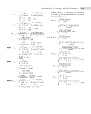
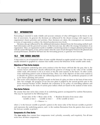
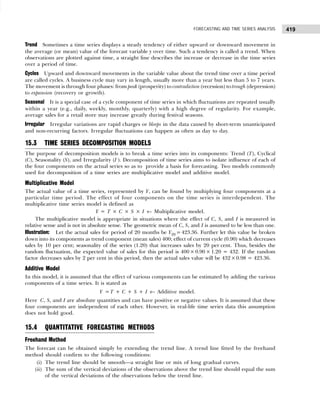
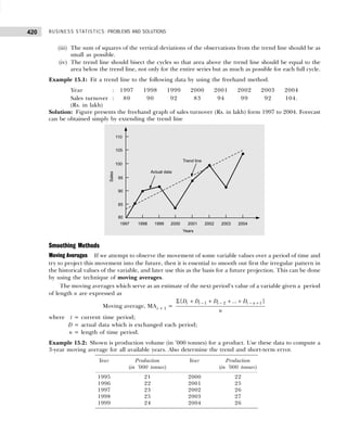
![421
FORECASTING AND TIME SERIES ANALYSIS
Solution: The first average is computed for the first 3 years as follows:
Moving average (year 1–3) =
21 22 23
3
+ +
= 22.
The first 3-year moving average can be used to forecast the production volume in fourth year, 1998.
Because 25,000 tonnes production was made in 1998, the error of the forecast is Error1998 = 25,000 –
22,000 = 3000 tonnes.
Similarly, the moving average calculation for the next 3 years is
Moving average (year 2–4) =
22 23 25
3
+ +
= 23.33.
A complete summary of 3-year moving average calculations is given in Table 15.1.
OddandEvenNumberofYears When the chosen period of length n is an odd number, the moving average period
is centred on i (middle period in the consecutive sequence of n periods). For instance, with n = 5, MA3(5) is
centred on the third year, MA4(5) is centred on the fourth year..., and MA9(5) is centred on the ninth year.
No moving average can be obtained for the first (n – 1)/2 years or the last (n – 1)/2 years of the series.
Thus, for a 5-year moving average, we cannot make computations for the just two years or the last two
years of the series.
When the chosen period of length n is an even numbers, equal parts can easily be formed and an
average of each part is obtained. For example, if n = 4, then the first moving average M3 (placed at
period 3) is an average of the first four data values and the second moving average M4 (placed at period 4)
is the average of data values 2 through 5. The average of M3 and M4 is placed at period 3 because it is an
average of data values for period 1 through 5.
Example 15.3: Assume a four-year cycle and calculate the trend by the method of moving average from
the following data relating to the production of tea in India:
[Madras, Univ., M.Com., 1997]
→
→
→
→
Table 15.1 Calculation of Trend and Short-term Fluctuations
Year Production 3-Year Moving 3-Yearly Moving Forecast Error
y Total Average ( y –
y )
(Trend values)
y
1995 21 — — —
1996 22 (21 + 22 + 23) = 66 66/3 = 22.00 0
1997 23 (22 + 23 + 25) = 70 70/3 = 23.33 – 0.33
1998 25 (23 + 25 + 24) = 72 72/3 = 24.00 1.00
1999 24 71 23.67 0.33
2000 22 71 23.67 – 1.67
2001 25 73 24.33 0.67
2002 26 78 26.00 0
2003 27 (26 + 27 + 26) = 79 79/3 = 26.33 0.67
2004 26 — — —
Year Production Year Production
(million lbs) (million lbs)
1987 464 1992 540
1988 515 1993 557
1989 518 1994 571
1990 467 1995 586
1991 502 1996 612](https://image.slidesharecdn.com/businessstatisticsproblemsandsolutions-230910073954-6d42a210/85/Business-Statistics_-Problems-and-Solutions-pdf-435-320.jpg)
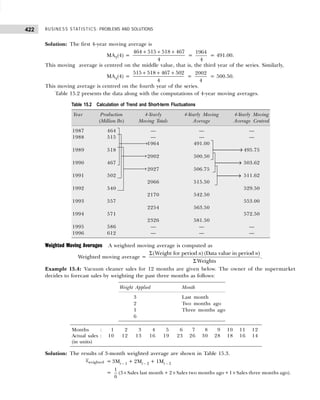
![423
FORECASTING AND TIME SERIES ANALYSIS
Example 15.5: A food processor uses a moving average to forecast next month’s demand. Past actual
demand (in units) is shown below:
Month : 43 44 45 46 47 48 49 50 51
Actual
demand : 105 106 110 110 114 121 130 128 137
(a) Compute a simple five-month moving average to forecast demand for month 52.
(b) Compute a weighted three-month moving average where the weights are highest for the latest months
and descend in order of 3, 2, 1.
Solution: Calculations for five-month moving average are shown in Table 15.4.
Table 15.3 Weighted Moving Average
Month Actual Sales Three-Month Weighted Moving Average
1 10 —
2 12 —
3 13 —
4 16
1
6
[(3 × 13) + (2 × 12) + (1 × 10)] =
121
6
5 19
1
6
[(3 × 16) + (2 × 13) + (1 × 12)] =
141
3
6 23
1
6
[(3 × 19) + (2 × 16) + (1 × 13)] = 17
7 26
1
6
[(3 × 23) + (2 × 19) + (1 × 16)] =
201
2
8 30
1
6
[(3 × 26) + (2 × 23) + (1 × 19)] =
235
6
9 28
1
6
[(3 × 30) + (2 × 26) + (1 × 23)] =
271
2
10 18
1
6
[(3 × 28) + (2 × 30) + (1 × 26)] =
289
3
11 16
1
6
[(3 × 18) + (2 × 28) + (1 × 30)] =
231
3
12 14
1
6
[(3 × 16) + (2 × 18) + (1 × 28)] =
182
3
Table 15.4 Five-month Moving Average
Month Actual Demand 5-Month 5-Month
Moving Total Moving Average
43 105 — —
44 106 — —
45 110 545 109.50
46 110 561 112.2
47 114 585 117.0
48 121 603 120.6
49 130 630 126.0
50 128 — —
51 137 — —](https://image.slidesharecdn.com/businessstatisticsproblemsandsolutions-230910073954-6d42a210/85/Business-Statistics_-Problems-and-Solutions-pdf-437-320.jpg)
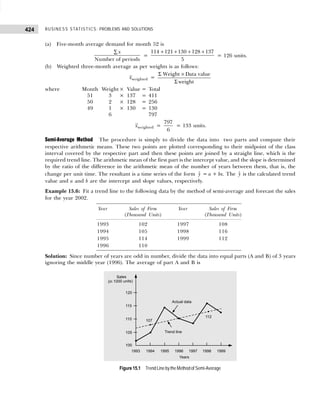
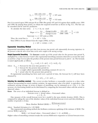
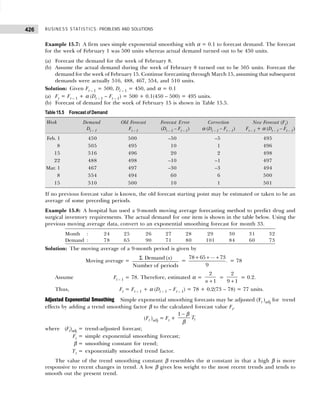
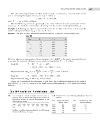
![BUSINESS STATISTICS: PROBLEMS AND SOLUTIONS
428
15.3 A State Govt. is studying the number of traffic fatalities
in the state resulting from drunken driving for each
of the last 12 months
Month Accidents
1 280
2 300
3 280
4 280
5 270
6 240
7 230
8 230
9 220
10 200
11 210
12 200
Find the trend line that describes the trend by using
the method of semi-averages.
15.4 Calculate the three-month moving averages from the
following data:
Jan. Feb. March April May June
57 65 63 72 69 78
July Aug. Sept. Oct. Nov. Dec.
82 81 90 92 95 97
[Osmania Univ., B.Com., 1996]
15.5 Gross revenue data (Rs. in million) for a Travel Agency
for a 11-year period is as follows:
Year Revenue
1995 3
1996 6
1997 1 0
1998 8
1999 7
2000 1 2
2001 1 4
2002 1 4
2003 1 8
2004 19
Calculate a 3-year moving average for the revenue
earned.
15.6 The owner of a small manufacturing company has
been concerned about the increase in manufacturing
costs over the past 10 years. The following data
provide a time series of the cost per unit for the
company’s leading product over the past 10 years.
Year Cost per Unit Year Cost per Unit
1995 332 2000 405
1996 317 2001 410
1997 357 2002 427
1998 392 2003 405
1999 402 2004 438
Calculate a 5-year moving average for the unit cost of
the product.
15.7 The following data provide a time series of the
number of Commercial and Industrial units failures
during the period 1989–2004.
Year No. of Failures Year No. of Failures
1989 23 1997 9
1990 26 1998 13
1991 28 1999 11
1992 32 2000 14
1993 20 2001 12
1994 12 2002 9
1995 12 2003 3
1996 10 2004 1
Calculate a 5-year and 7-year moving average for the
number of units failure.
15.8 Estimate the trend values using the data given by
taking a four-year moving average:
Year Value Year Value
1990 12 1997 100
1991 25 1998 82
1992 39 1999 65
1993 54 2000 49
1994 70 2001 34
1995 87 2002 20
1996 105 2003 7
[Madras Univ., M.Com., 1998]
15.9 In January, a city hotel predicted a February demand
for 142 room occupancy. Actual February demand was
153 rooms. Using a smoothing constant of α = 0.20,
forecast the March demand using the exponential
smoothing model.
15.10 A shoe manufacturer, using exponential smoothing
with α = 0.1, has developed a January trend forecast
of 400 units for a ladies' shoe. This brand has seasonal
indexes of 0.80, 0.90, and 1.20, respectively, for the
first three months of the year. Assuming actual sales
were 344 units in January and 414 units in February,
what would be the seasonalized March forecast?
15.11 A food processor uses exponential smoothing (with
α = 0.10) to forecast next month’s demand. Past
(actual) demand in units and the simple exponential
forecasts up to month 51 are shown in the following
table:](https://image.slidesharecdn.com/businessstatisticsproblemsandsolutions-230910073954-6d42a210/85/Business-Statistics_-Problems-and-Solutions-pdf-442-320.jpg)
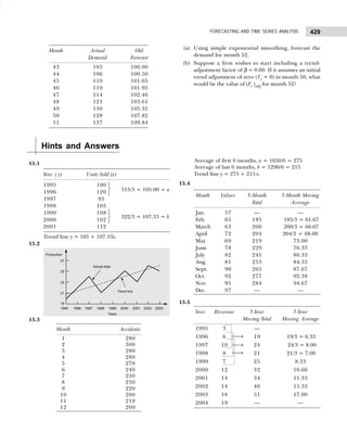
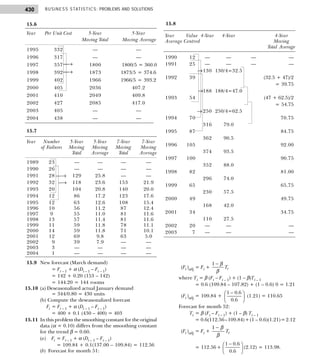
![431
FORECASTING AND TIME SERIES ANALYSIS
15.5 TREND PROJECTION METHODS
The trend projection method fits a trend line to a time series data and then projects medium-to-long-
range forecasts. Several possible trend fits can be explored (such as exponential and quadratic), depending
upon movement of time series data.
Linear Trend Model
The method of least squares from regression analysis is used to find the trend line of best fit to a time series
data. The regression trend line (y) is defined by the following equation.
ŷ = a + bx
where ŷ = predicted value of the dependent variable;
a = y-axis intercept;
b = slope of the regression line (or the rate of change in y for a given change in x);
x = independent variable (which is time in this case).
The values of constants a and b can be obtained by solving normal equations
Σ y = na + bΣ x and Σxy = aΣx + bΣx2
where the data can be coded so that Σ x = 0, two terms in these equations drop out and we have
Σ y = na and Σ x y = bΣx2
.
Alternately, we can also find the values of constants a and b for any regression line as
b =
Σ −
Σ −
2 2
( )
x y n x y
x n x
and a = −
y b x.
Example 15.10: Below are given the figures of production (in thousand quintals) of a sugar factory:
Year : 1995 1996 1997 1998 1999 2000 2001
Production : 80 90 92 83 94 99 92
(a) Fit a straight line trend to these figures.
(b) Plot these figures on a graph and show the trend line.
(c) Estimate the production in 2004. [Bangalore Univ., B.Com., 1998]
Solution: (a) Using normal equations and the sugar production data we can compute constants a and b as
shown in Table 15.7:
x =
x
n
Σ
=
28
7
= 4, y =
y
n
Σ
=
630
7
= 90
b = 2 2
( )
x y n x y
x n x
Σ −
Σ −
=
−
− 2
2576 7(4) (90)
140 7(4)
=
56
28
= 2
a = y – b x = 90 – 2(4) = 82.
Table 15.7 Calculation for Least Squares Equation
Year Time Period Production x2
xy Trend Values
(x) (x) (
y)
1995 1 80 1 80 84
1996 2 90 4 180 86
1997 3 92 9 276 88
1998 4 83 16 332 90
1999 5 94 25 470 92
2000 6 99 36 594 94
2001 7 92 49 644 96
28 630 140 2576](https://image.slidesharecdn.com/businessstatisticsproblemsandsolutions-230910073954-6d42a210/85/Business-Statistics_-Problems-and-Solutions-pdf-445-320.jpg)
![BUSINESS STATISTICS: PROBLEMS AND SOLUTIONS
432
Figure15.2 LinearTrendforProductionofSugar
Therefore, linear trend component for the production of sugar is
ŷ = a + bx = 82 + 2x.
The slope b = 2 indicates that over the past 7 years, the production of sugar had an average growth of
about 2 thousand quintals per year.
(b) Plotting points on the graph paper, we get an actual graph representing production of sugar over the
past 7 years. On joining the points a = 82 and b = 2 (corresponds to 1996) on the graph we get a trend
line as shown in Fig. 15.2.
(c) The production of sugar for year 2004 will be
ŷ = a + bx = 82 + 2x.
Example 15.11: The following table relates to the tourist arrivals (in millions) during 1994 to 2000 in
India:
Year : 1994 1995 1996 1997 1998 1999 2000
Tourists arrivals : 18 20 23 25 24 28 30
Fit a straight line trend by the method of least squares and estimate the number of tourists that would
arrive in the year 2004. [Kurukshetra Univ., MTM, 1997]
Solution: Using normal equations and the tourists arrival data we can compute constants a and b as
shown in Table 15.8:
Table 15.8 Calculations for Least Squares Equation
Year Time Tourist
Scale Arrivals
(x) y xy x2
1994 –3 18 –54 9
1995 –2 20 –40 4
1996 –1 23 –23 1
1997 0 25 0 0
1998 1 24 24 1
1999 2 28 56 4
2000 3 30 90 9
168 53 28](https://image.slidesharecdn.com/businessstatisticsproblemsandsolutions-230910073954-6d42a210/85/Business-Statistics_-Problems-and-Solutions-pdf-446-320.jpg)