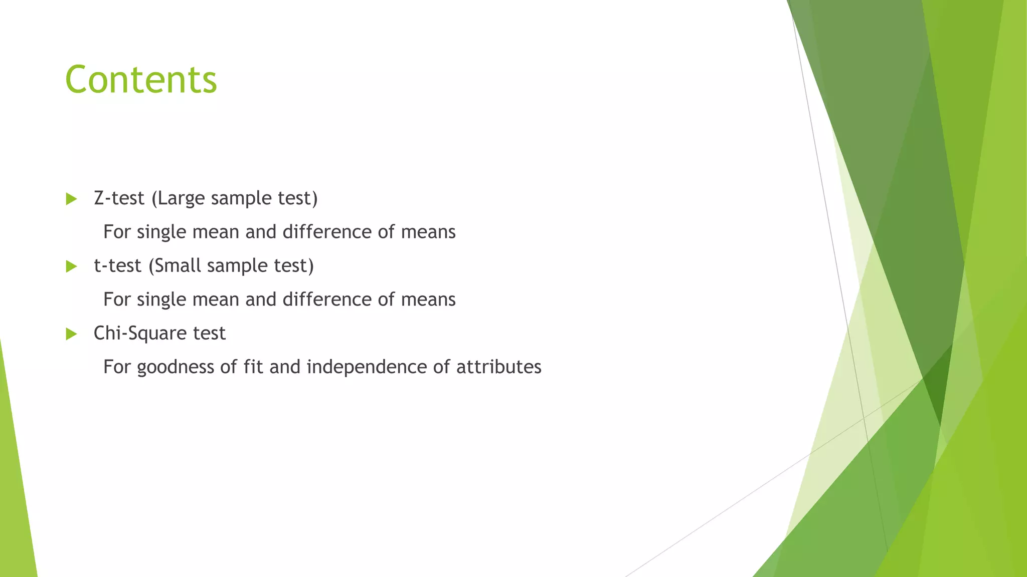
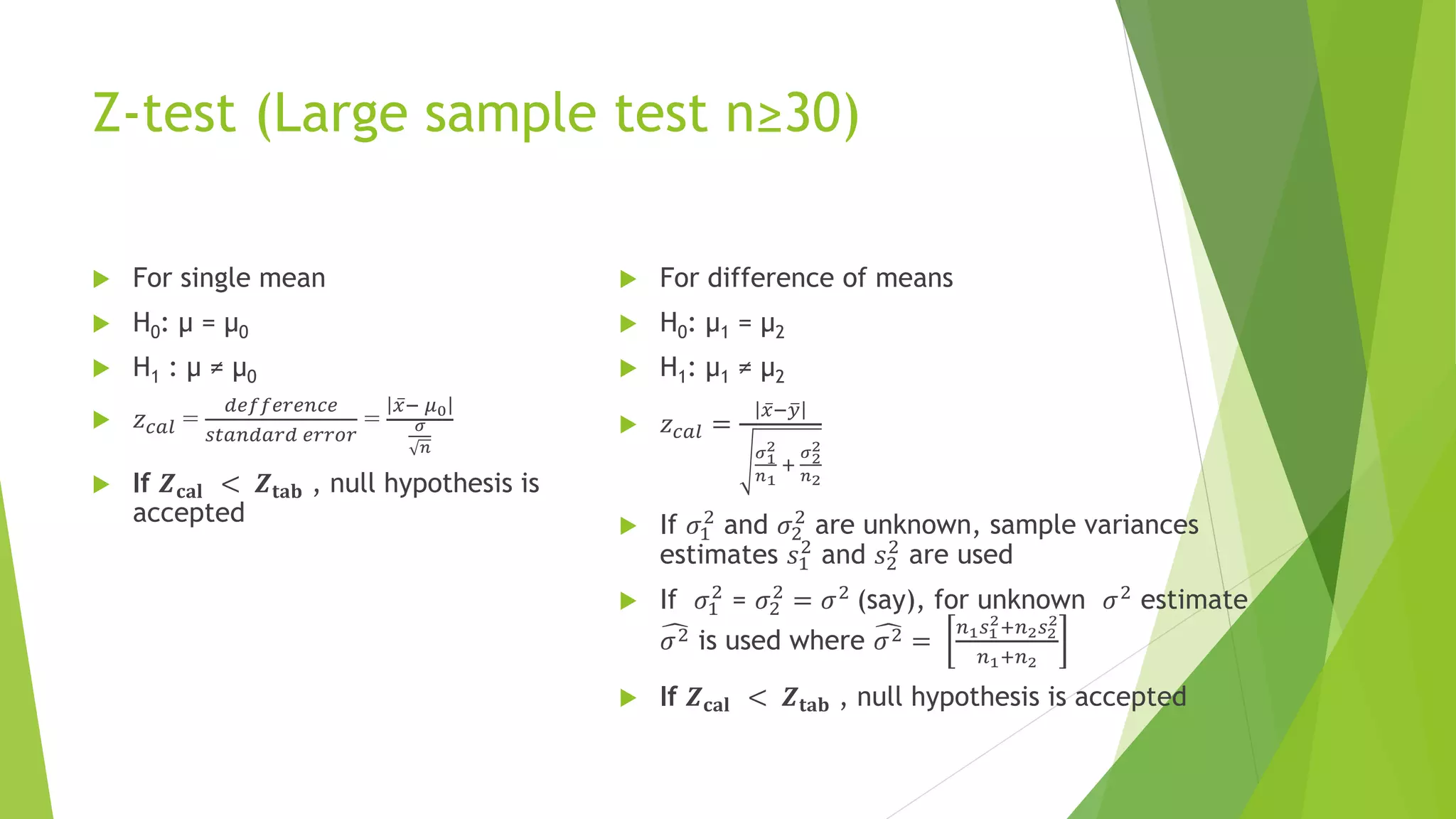
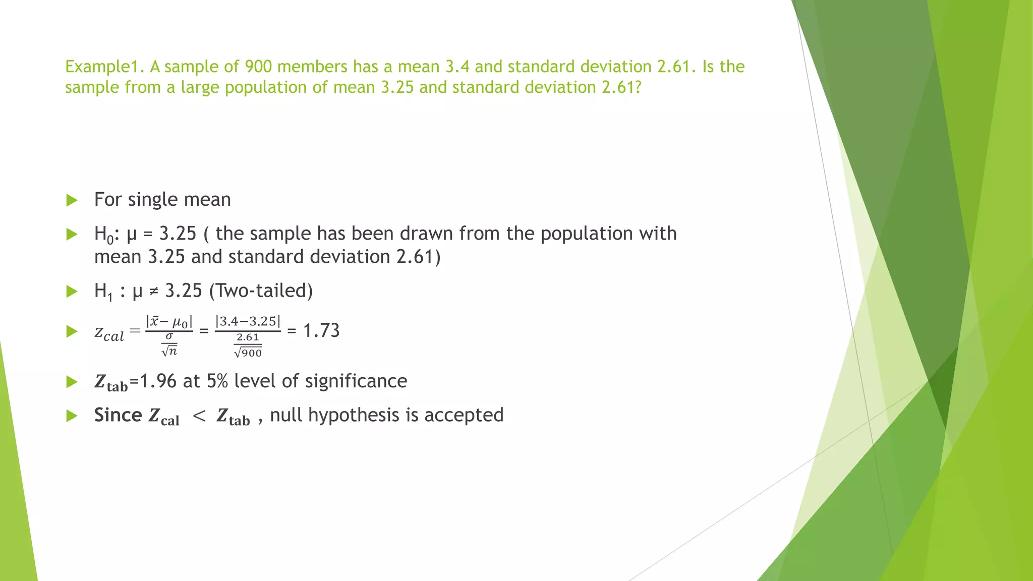
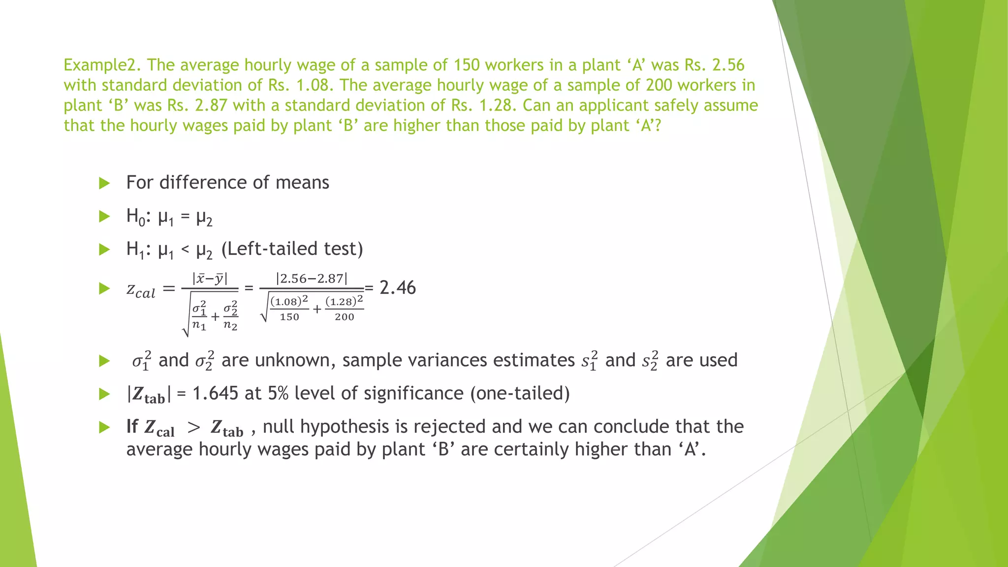
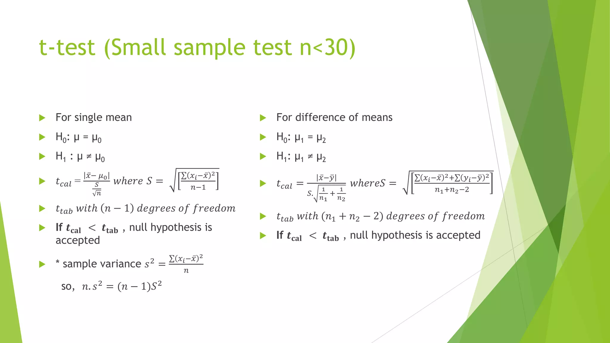
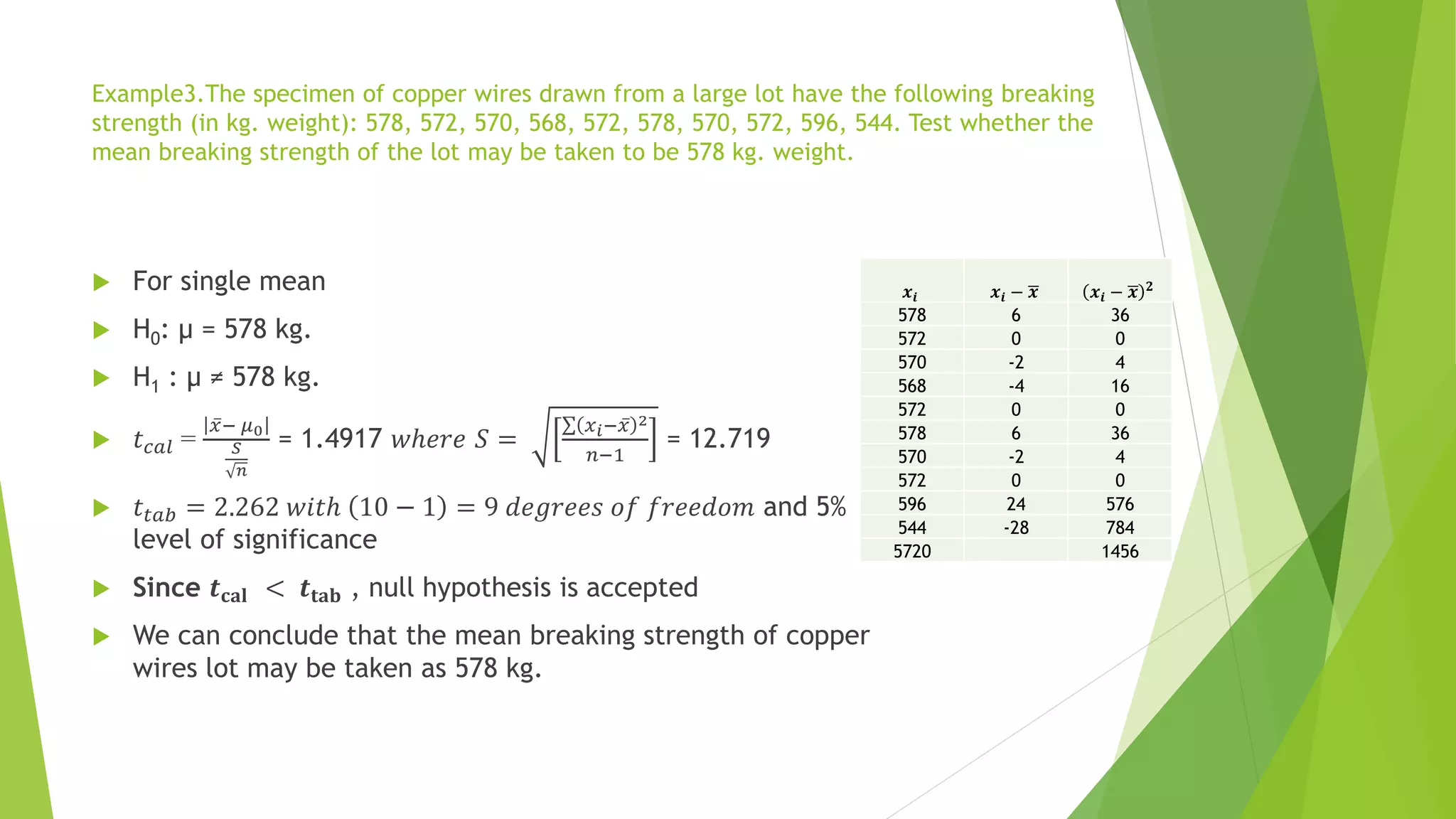
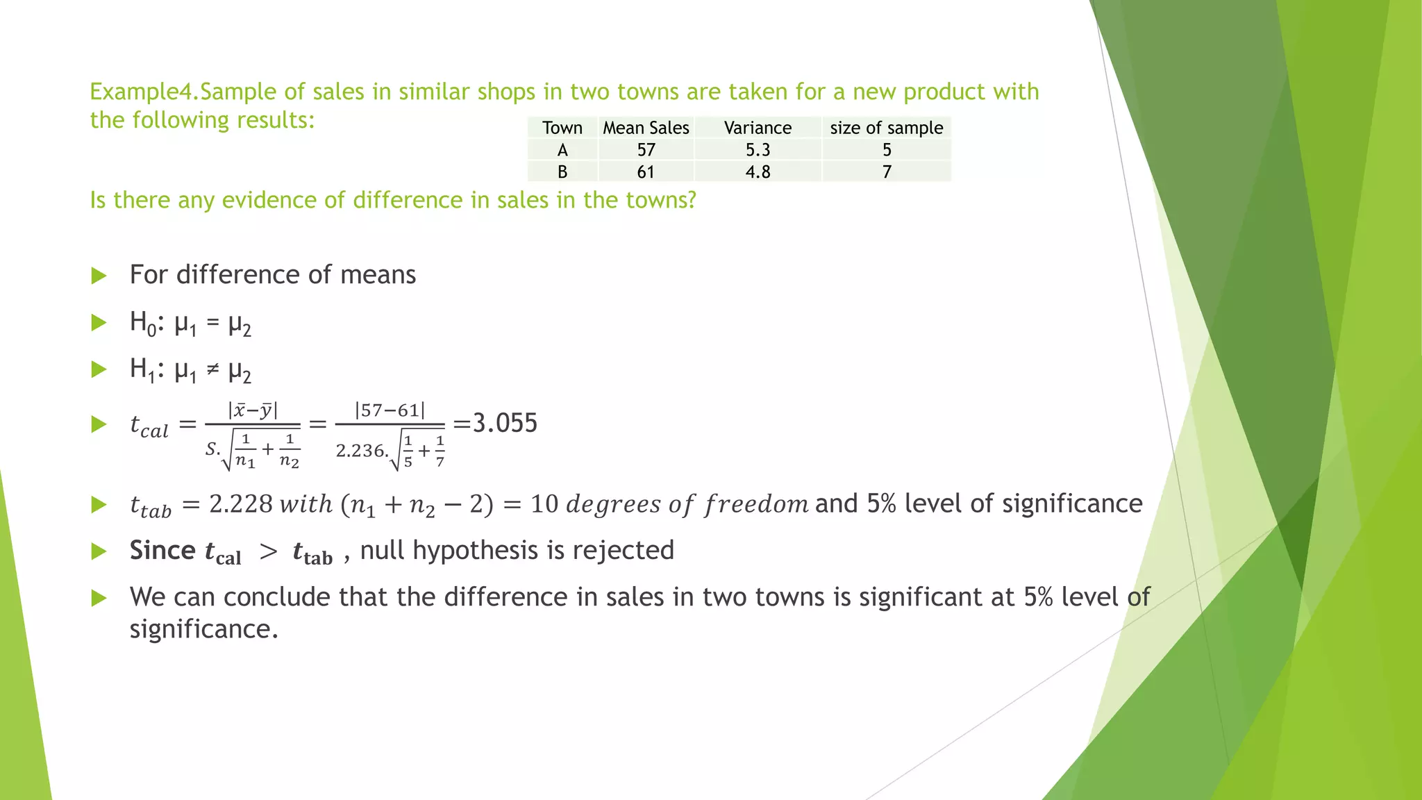
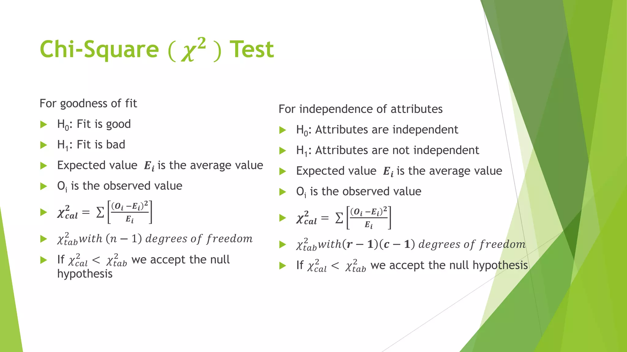
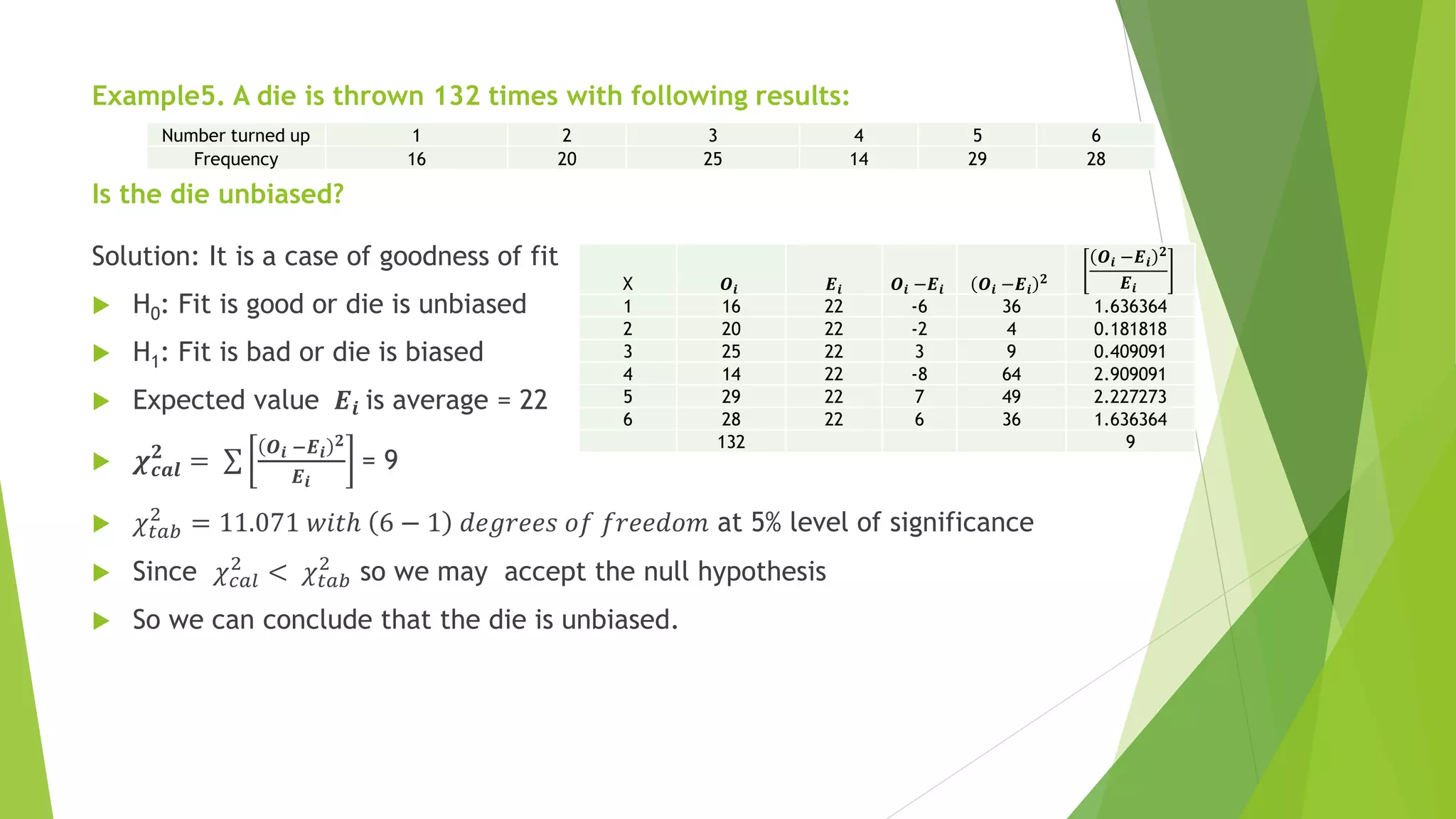
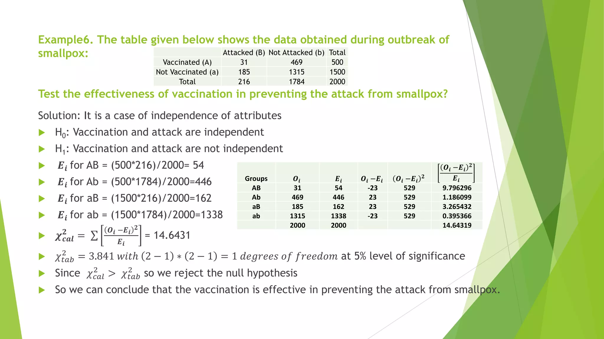
Inferential Test Procedures
Probability and Statistics (MA202): Unit V
Department of Applied Sciences, DIT University Dehradun
Contents
 Z-test (Large sample test)
For single mean and difference of means
 t-test (Small sample test)
For single mean and difference of means
 Chi-Square test
For goodness of fit and independence of attributes
Z-test (Large sample test n≥30)
 For single mean
 H0: µ = µ0
 H1 : µ ≠ µ0
 𝑧𝑐𝑎𝑙 =
𝑑𝑒𝑓𝑓𝑒𝑟𝑒𝑛𝑐𝑒
𝑠𝑡𝑎𝑛𝑑𝑎𝑟𝑑 𝑒𝑟𝑟𝑜𝑟
=
ҧ
𝑥− 𝜇0
𝜎
𝑛
 If 𝒁𝐜𝐚𝐥 < 𝒁𝐭𝐚𝐛 , null hypothesis is
accepted
 For difference of means
 H0: µ1 = µ2
 H1: µ1 ≠ µ2
 𝑧𝑐𝑎𝑙 =
ҧ
𝑥− ത
𝑦
𝜎1
2
𝑛1
+
𝜎2
2
𝑛2
 If 𝜎1
2
and 𝜎2
2
are unknown, sample variances
estimates 𝑠1
2
and 𝑠2
2
are used
 If 𝜎1
2
= 𝜎2
2
= 𝜎2
(say), for unknown 𝜎2
estimate
෢
𝜎2 is used where ෢
𝜎2 =
𝑛1𝑠1
2+𝑛2𝑠2
2
𝑛1+𝑛2
 If 𝒁𝐜𝐚𝐥 < 𝒁𝐭𝐚𝐛 , null hypothesis is accepted
Example1. A sample of 900 members has a mean 3.4 and standard deviation 2.61. Is the
sample from a large population of mean 3.25 and standard deviation 2.61?
 For single mean
 H0: µ = 3.25 ( the sample has been drawn from the population with
mean 3.25 and standard deviation 2.61)
 H1 : µ ≠ 3.25 (Two-tailed)
 𝑧𝑐𝑎𝑙 =
ҧ
𝑥− 𝜇0
𝜎
𝑛
=
3.4−3.25
2.61
900
= 1.73
 𝒁𝐭𝐚𝐛=1.96 at 5% level of significance
 Since 𝒁𝐜𝐚𝐥 < 𝒁𝐭𝐚𝐛 , null hypothesis is accepted
Example2. The average hourly wage of a sample of 150 workers in a plant ‘A’ was Rs. 2.56
with standard deviation of Rs. 1.08. The average hourly wage of a sample of 200 workers in
plant ‘B’ was Rs. 2.87 with a standard deviation of Rs. 1.28. Can an applicant safely assume
that the hourly wages paid by plant ‘B’ are higher than those paid by plant ‘A’?
 For difference of means
 H0: µ1 = µ2
 H1: µ1 < µ2 (Left-tailed test)
 𝑧𝑐𝑎𝑙 =
ҧ
𝑥− ത
𝑦
𝜎1
2
𝑛1
+
𝜎2
2
𝑛2
=
2.56−2.87
1.08 2
150
+
1.28 2
200
= 2.46
 𝜎1
2
and 𝜎2
2
are unknown, sample variances estimates 𝑠1
2
and 𝑠2
2
are used
 𝒁𝐭𝐚𝐛 = 1.645 at 5% level of significance (one-tailed)
 If 𝒁𝐜𝐚𝐥 > 𝒁𝐭𝐚𝐛 , null hypothesis is rejected and we can conclude that the
average hourly wages paid by plant ‘B’ are certainly higher than ‘A’.
t-test (Small sample test n<30)
 For single mean
 H0: µ = µ0
 H1 : µ ≠ µ0
 𝑡𝑐𝑎𝑙 =
ҧ
𝑥− 𝜇0
𝑆
𝑛
𝑤ℎ𝑒𝑟𝑒 𝑆 =
σ 𝑥𝑖− ҧ
𝑥 2
𝑛−1
 𝑡𝑡𝑎𝑏 𝑤𝑖𝑡ℎ 𝑛 − 1 𝑑𝑒𝑔𝑟𝑒𝑒𝑠 𝑜𝑓 𝑓𝑟𝑒𝑒𝑑𝑜𝑚
 If 𝒕𝐜𝐚𝐥 < 𝒕𝐭𝐚𝐛 , null hypothesis is
accepted
 * sample variance 𝑠2
=
σ 𝑥𝑖− ҧ
𝑥 2
𝑛
so, 𝑛. 𝑠2
= (𝑛 − 1)𝑆2
 For difference of means
 H0: µ1 = µ2
 H1: µ1 ≠ µ2
 𝑡𝑐𝑎𝑙 =
ҧ
𝑥− ത
𝑦
𝑆.
1
𝑛1
+
1
𝑛2
𝑤ℎ𝑒𝑟𝑒𝑆 =
σ 𝑥𝑖− ҧ
𝑥 2+σ 𝑦𝑖− ത
𝑦 2
𝑛1+𝑛2−2
 𝑡𝑡𝑎𝑏 𝑤𝑖𝑡ℎ (𝑛1 + 𝑛2 − 2) 𝑑𝑒𝑔𝑟𝑒𝑒𝑠 𝑜𝑓 𝑓𝑟𝑒𝑒𝑑𝑜𝑚
 If 𝒕𝐜𝐚𝐥 < 𝒕𝐭𝐚𝐛 , null hypothesis is accepted
Example3.The specimen of copper wires drawn from a large lot have the following breaking
strength (in kg. weight): 578, 572, 570, 568, 572, 578, 570, 572, 596, 544. Test whether the
mean breaking strength of the lot may be taken to be 578 kg. weight.
 For single mean
 H0: µ = 578 kg.
 H1 : µ ≠ 578 kg.
 𝑡𝑐𝑎𝑙 =
ҧ
𝑥− 𝜇0
𝑆
𝑛
= 1.4917 𝑤ℎ𝑒𝑟𝑒 𝑆 =
σ 𝑥𝑖− ҧ
𝑥 2
𝑛−1
= 12.719
 𝑡𝑡𝑎𝑏 = 2.262 𝑤𝑖𝑡ℎ 10 − 1 = 9 𝑑𝑒𝑔𝑟𝑒𝑒𝑠 𝑜𝑓 𝑓𝑟𝑒𝑒𝑑𝑜𝑚 and 5%
level of significance
 Since 𝒕𝐜𝐚𝐥 < 𝒕𝐭𝐚𝐛 , null hypothesis is accepted
 We can conclude that the mean breaking strength of copper
wires lot may be taken as 578 kg.
𝒙𝒊 𝒙𝒊 − ഥ
𝒙 𝒙𝒊 − ഥ
𝒙 𝟐
578 6 36
572 0 0
570 -2 4
568 -4 16
572 0 0
578 6 36
570 -2 4
572 0 0
596 24 576
544 -28 784
5720 1456
Example4.Sample of sales in similar shops in two towns are taken for a new product with
the following results:
Is there any evidence of difference in sales in the towns?
 For difference of means
 H0: µ1 = µ2
 H1: µ1 ≠ µ2
 𝑡𝑐𝑎𝑙 =
ҧ
𝑥− ത
𝑦
𝑆.
1
𝑛1
+
1
𝑛2
=
57−61
2.236.
1
5
+
1
7
=3.055
 𝑡𝑡𝑎𝑏 = 2.228 𝑤𝑖𝑡ℎ (𝑛1 + 𝑛2 − 2) = 10 𝑑𝑒𝑔𝑟𝑒𝑒𝑠 𝑜𝑓 𝑓𝑟𝑒𝑒𝑑𝑜𝑚 and 5% level of significance
 Since 𝒕𝐜𝐚𝐥 > 𝒕𝐭𝐚𝐛 , null hypothesis is rejected
 We can conclude that the difference in sales in two towns is significant at 5% level of
significance.
Town Mean Sales Variance size of sample
A 57 5.3 5
B 61 4.8 7
Chi-Square ( 𝝌𝟐
) Test
For goodness of fit
 H0: Fit is good
 H1: Fit is bad
 Expected value 𝑬𝒊 is the average value
 Oi is the observed value
 𝝌𝒄𝒂𝒍
𝟐
= σ
𝑶𝒊 −𝑬𝒊
𝟐
𝑬𝒊
 𝜒𝑡𝑎𝑏
2
𝑤𝑖𝑡ℎ 𝑛 − 1 𝑑𝑒𝑔𝑟𝑒𝑒𝑠 𝑜𝑓 𝑓𝑟𝑒𝑒𝑑𝑜𝑚
 If 𝜒𝑐𝑎𝑙
2
< 𝜒𝑡𝑎𝑏
2
we accept the null
hypothesis
For independence of attributes
 H0: Attributes are independent
 H1: Attributes are not independent
 Expected value 𝑬𝒊 is the average value
 Oi is the observed value
 𝝌𝒄𝒂𝒍
𝟐
= σ
𝑶𝒊 −𝑬𝒊
𝟐
𝑬𝒊
 𝜒𝑡𝑎𝑏
2
𝑤𝑖𝑡ℎ 𝒓 − 𝟏 𝒄 − 𝟏 𝑑𝑒𝑔𝑟𝑒𝑒𝑠 𝑜𝑓 𝑓𝑟𝑒𝑒𝑑𝑜𝑚
 If 𝜒𝑐𝑎𝑙
2
< 𝜒𝑡𝑎𝑏
2
we accept the null hypothesis
Example5. A die is thrown 132 times with following results:
Is the die unbiased?
Solution: It is a case of goodness of fit
 H0: Fit is good or die is unbiased
 H1: Fit is bad or die is biased
 Expected value 𝑬𝒊 is average = 22
 𝝌𝒄𝒂𝒍
𝟐
= σ
𝑶𝒊 −𝑬𝒊
𝟐
𝑬𝒊
= 9
 𝜒𝑡𝑎𝑏
2
= 11.071 𝑤𝑖𝑡ℎ 6 − 1 𝑑𝑒𝑔𝑟𝑒𝑒𝑠 𝑜𝑓 𝑓𝑟𝑒𝑒𝑑𝑜𝑚 at 5% level of significance
 Since 𝜒𝑐𝑎𝑙
2
< 𝜒𝑡𝑎𝑏
2
so we may accept the null hypothesis
 So we can conclude that the die is unbiased.
X 𝑶𝒊 𝑬𝒊 𝑶𝒊 −𝑬𝒊 𝑶𝒊 −𝑬𝒊
𝟐
𝑶𝒊 −𝑬𝒊
𝟐
𝑬𝒊
1 16 22 -6 36 1.636364
2 20 22 -2 4 0.181818
3 25 22 3 9 0.409091
4 14 22 -8 64 2.909091
5 29 22 7 49 2.227273
6 28 22 6 36 1.636364
132 9
Number turned up 1 2 3 4 5 6
Frequency 16 20 25 14 29 28
Example6. The table given below shows the data obtained during outbreak of
smallpox:
Test the effectiveness of vaccination in preventing the attack from smallpox?
Solution: It is a case of independence of attributes
 H0: Vaccination and attack are independent
 H1: Vaccination and attack are not independent
 𝑬𝒊 for AB = (500*216)/2000= 54
 𝑬𝒊 for Ab = (500*1784)/2000=446
 𝑬𝒊 for aB = (1500*216)/2000=162
 𝑬𝒊 for ab = (1500*1784)/2000=1338
 𝝌𝒄𝒂𝒍
𝟐
= σ
𝑶𝒊 −𝑬𝒊
𝟐
𝑬𝒊
= 14.6431
 𝜒𝑡𝑎𝑏
2
= 3.841 𝑤𝑖𝑡ℎ 2 − 1 ∗ 2 − 1 = 1 𝑑𝑒𝑔𝑟𝑒𝑒𝑠 𝑜𝑓 𝑓𝑟𝑒𝑒𝑑𝑜𝑚 at 5% level of significance
 Since 𝜒𝑐𝑎𝑙
2
> 𝜒𝑡𝑎𝑏
2
so we reject the null hypothesis
 So we can conclude that the vaccination is effective in preventing the attack from smallpox.
Groups 𝑶𝒊 𝑬𝒊 𝑶𝒊 −𝑬𝒊 𝑶𝒊 −𝑬𝒊
𝟐
𝑶𝒊 −𝑬𝒊
𝟐
𝑬𝒊
AB 31 54 -23 529 9.796296
Ab 469 446 23 529 1.186099
aB 185 162 23 529 3.265432
ab 1315 1338 -23 529 0.395366
2000 2000 14.64319
Attacked (B) Not Attacked (b) Total
Vaccinated (A) 31 469 500
Not Vaccinated (a) 185 1315 1500
Total 216 1784 2000
Thank You

t-z-chi-square tests of sig.pdf

  • 1.
    Inferential Test Procedures Probabilityand Statistics (MA202): Unit V Department of Applied Sciences, DIT University Dehradun
  • 2.
    Contents  Z-test (Largesample test) For single mean and difference of means  t-test (Small sample test) For single mean and difference of means  Chi-Square test For goodness of fit and independence of attributes
  • 3.
    Z-test (Large sampletest n≥30)  For single mean  H0: µ = µ0  H1 : µ ≠ µ0  𝑧𝑐𝑎𝑙 = 𝑑𝑒𝑓𝑓𝑒𝑟𝑒𝑛𝑐𝑒 𝑠𝑡𝑎𝑛𝑑𝑎𝑟𝑑 𝑒𝑟𝑟𝑜𝑟 = ҧ 𝑥− 𝜇0 𝜎 𝑛  If 𝒁𝐜𝐚𝐥 < 𝒁𝐭𝐚𝐛 , null hypothesis is accepted  For difference of means  H0: µ1 = µ2  H1: µ1 ≠ µ2  𝑧𝑐𝑎𝑙 = ҧ 𝑥− ത 𝑦 𝜎1 2 𝑛1 + 𝜎2 2 𝑛2  If 𝜎1 2 and 𝜎2 2 are unknown, sample variances estimates 𝑠1 2 and 𝑠2 2 are used  If 𝜎1 2 = 𝜎2 2 = 𝜎2 (say), for unknown 𝜎2 estimate ෢ 𝜎2 is used where ෢ 𝜎2 = 𝑛1𝑠1 2+𝑛2𝑠2 2 𝑛1+𝑛2  If 𝒁𝐜𝐚𝐥 < 𝒁𝐭𝐚𝐛 , null hypothesis is accepted
  • 4.
    Example1. A sampleof 900 members has a mean 3.4 and standard deviation 2.61. Is the sample from a large population of mean 3.25 and standard deviation 2.61?  For single mean  H0: µ = 3.25 ( the sample has been drawn from the population with mean 3.25 and standard deviation 2.61)  H1 : µ ≠ 3.25 (Two-tailed)  𝑧𝑐𝑎𝑙 = ҧ 𝑥− 𝜇0 𝜎 𝑛 = 3.4−3.25 2.61 900 = 1.73  𝒁𝐭𝐚𝐛=1.96 at 5% level of significance  Since 𝒁𝐜𝐚𝐥 < 𝒁𝐭𝐚𝐛 , null hypothesis is accepted
  • 5.
    Example2. The averagehourly wage of a sample of 150 workers in a plant ‘A’ was Rs. 2.56 with standard deviation of Rs. 1.08. The average hourly wage of a sample of 200 workers in plant ‘B’ was Rs. 2.87 with a standard deviation of Rs. 1.28. Can an applicant safely assume that the hourly wages paid by plant ‘B’ are higher than those paid by plant ‘A’?  For difference of means  H0: µ1 = µ2  H1: µ1 < µ2 (Left-tailed test)  𝑧𝑐𝑎𝑙 = ҧ 𝑥− ത 𝑦 𝜎1 2 𝑛1 + 𝜎2 2 𝑛2 = 2.56−2.87 1.08 2 150 + 1.28 2 200 = 2.46  𝜎1 2 and 𝜎2 2 are unknown, sample variances estimates 𝑠1 2 and 𝑠2 2 are used  𝒁𝐭𝐚𝐛 = 1.645 at 5% level of significance (one-tailed)  If 𝒁𝐜𝐚𝐥 > 𝒁𝐭𝐚𝐛 , null hypothesis is rejected and we can conclude that the average hourly wages paid by plant ‘B’ are certainly higher than ‘A’.
  • 6.
    t-test (Small sampletest n<30)  For single mean  H0: µ = µ0  H1 : µ ≠ µ0  𝑡𝑐𝑎𝑙 = ҧ 𝑥− 𝜇0 𝑆 𝑛 𝑤ℎ𝑒𝑟𝑒 𝑆 = σ 𝑥𝑖− ҧ 𝑥 2 𝑛−1  𝑡𝑡𝑎𝑏 𝑤𝑖𝑡ℎ 𝑛 − 1 𝑑𝑒𝑔𝑟𝑒𝑒𝑠 𝑜𝑓 𝑓𝑟𝑒𝑒𝑑𝑜𝑚  If 𝒕𝐜𝐚𝐥 < 𝒕𝐭𝐚𝐛 , null hypothesis is accepted  * sample variance 𝑠2 = σ 𝑥𝑖− ҧ 𝑥 2 𝑛 so, 𝑛. 𝑠2 = (𝑛 − 1)𝑆2  For difference of means  H0: µ1 = µ2  H1: µ1 ≠ µ2  𝑡𝑐𝑎𝑙 = ҧ 𝑥− ത 𝑦 𝑆. 1 𝑛1 + 1 𝑛2 𝑤ℎ𝑒𝑟𝑒𝑆 = σ 𝑥𝑖− ҧ 𝑥 2+σ 𝑦𝑖− ത 𝑦 2 𝑛1+𝑛2−2  𝑡𝑡𝑎𝑏 𝑤𝑖𝑡ℎ (𝑛1 + 𝑛2 − 2) 𝑑𝑒𝑔𝑟𝑒𝑒𝑠 𝑜𝑓 𝑓𝑟𝑒𝑒𝑑𝑜𝑚  If 𝒕𝐜𝐚𝐥 < 𝒕𝐭𝐚𝐛 , null hypothesis is accepted
  • 7.
    Example3.The specimen ofcopper wires drawn from a large lot have the following breaking strength (in kg. weight): 578, 572, 570, 568, 572, 578, 570, 572, 596, 544. Test whether the mean breaking strength of the lot may be taken to be 578 kg. weight.  For single mean  H0: µ = 578 kg.  H1 : µ ≠ 578 kg.  𝑡𝑐𝑎𝑙 = ҧ 𝑥− 𝜇0 𝑆 𝑛 = 1.4917 𝑤ℎ𝑒𝑟𝑒 𝑆 = σ 𝑥𝑖− ҧ 𝑥 2 𝑛−1 = 12.719  𝑡𝑡𝑎𝑏 = 2.262 𝑤𝑖𝑡ℎ 10 − 1 = 9 𝑑𝑒𝑔𝑟𝑒𝑒𝑠 𝑜𝑓 𝑓𝑟𝑒𝑒𝑑𝑜𝑚 and 5% level of significance  Since 𝒕𝐜𝐚𝐥 < 𝒕𝐭𝐚𝐛 , null hypothesis is accepted  We can conclude that the mean breaking strength of copper wires lot may be taken as 578 kg. 𝒙𝒊 𝒙𝒊 − ഥ 𝒙 𝒙𝒊 − ഥ 𝒙 𝟐 578 6 36 572 0 0 570 -2 4 568 -4 16 572 0 0 578 6 36 570 -2 4 572 0 0 596 24 576 544 -28 784 5720 1456
  • 8.
    Example4.Sample of salesin similar shops in two towns are taken for a new product with the following results: Is there any evidence of difference in sales in the towns?  For difference of means  H0: µ1 = µ2  H1: µ1 ≠ µ2  𝑡𝑐𝑎𝑙 = ҧ 𝑥− ത 𝑦 𝑆. 1 𝑛1 + 1 𝑛2 = 57−61 2.236. 1 5 + 1 7 =3.055  𝑡𝑡𝑎𝑏 = 2.228 𝑤𝑖𝑡ℎ (𝑛1 + 𝑛2 − 2) = 10 𝑑𝑒𝑔𝑟𝑒𝑒𝑠 𝑜𝑓 𝑓𝑟𝑒𝑒𝑑𝑜𝑚 and 5% level of significance  Since 𝒕𝐜𝐚𝐥 > 𝒕𝐭𝐚𝐛 , null hypothesis is rejected  We can conclude that the difference in sales in two towns is significant at 5% level of significance. Town Mean Sales Variance size of sample A 57 5.3 5 B 61 4.8 7
  • 9.
    Chi-Square ( 𝝌𝟐 )Test For goodness of fit  H0: Fit is good  H1: Fit is bad  Expected value 𝑬𝒊 is the average value  Oi is the observed value  𝝌𝒄𝒂𝒍 𝟐 = σ 𝑶𝒊 −𝑬𝒊 𝟐 𝑬𝒊  𝜒𝑡𝑎𝑏 2 𝑤𝑖𝑡ℎ 𝑛 − 1 𝑑𝑒𝑔𝑟𝑒𝑒𝑠 𝑜𝑓 𝑓𝑟𝑒𝑒𝑑𝑜𝑚  If 𝜒𝑐𝑎𝑙 2 < 𝜒𝑡𝑎𝑏 2 we accept the null hypothesis For independence of attributes  H0: Attributes are independent  H1: Attributes are not independent  Expected value 𝑬𝒊 is the average value  Oi is the observed value  𝝌𝒄𝒂𝒍 𝟐 = σ 𝑶𝒊 −𝑬𝒊 𝟐 𝑬𝒊  𝜒𝑡𝑎𝑏 2 𝑤𝑖𝑡ℎ 𝒓 − 𝟏 𝒄 − 𝟏 𝑑𝑒𝑔𝑟𝑒𝑒𝑠 𝑜𝑓 𝑓𝑟𝑒𝑒𝑑𝑜𝑚  If 𝜒𝑐𝑎𝑙 2 < 𝜒𝑡𝑎𝑏 2 we accept the null hypothesis
  • 10.
    Example5. A dieis thrown 132 times with following results: Is the die unbiased? Solution: It is a case of goodness of fit  H0: Fit is good or die is unbiased  H1: Fit is bad or die is biased  Expected value 𝑬𝒊 is average = 22  𝝌𝒄𝒂𝒍 𝟐 = σ 𝑶𝒊 −𝑬𝒊 𝟐 𝑬𝒊 = 9  𝜒𝑡𝑎𝑏 2 = 11.071 𝑤𝑖𝑡ℎ 6 − 1 𝑑𝑒𝑔𝑟𝑒𝑒𝑠 𝑜𝑓 𝑓𝑟𝑒𝑒𝑑𝑜𝑚 at 5% level of significance  Since 𝜒𝑐𝑎𝑙 2 < 𝜒𝑡𝑎𝑏 2 so we may accept the null hypothesis  So we can conclude that the die is unbiased. X 𝑶𝒊 𝑬𝒊 𝑶𝒊 −𝑬𝒊 𝑶𝒊 −𝑬𝒊 𝟐 𝑶𝒊 −𝑬𝒊 𝟐 𝑬𝒊 1 16 22 -6 36 1.636364 2 20 22 -2 4 0.181818 3 25 22 3 9 0.409091 4 14 22 -8 64 2.909091 5 29 22 7 49 2.227273 6 28 22 6 36 1.636364 132 9 Number turned up 1 2 3 4 5 6 Frequency 16 20 25 14 29 28
  • 11.
    Example6. The tablegiven below shows the data obtained during outbreak of smallpox: Test the effectiveness of vaccination in preventing the attack from smallpox? Solution: It is a case of independence of attributes  H0: Vaccination and attack are independent  H1: Vaccination and attack are not independent  𝑬𝒊 for AB = (500*216)/2000= 54  𝑬𝒊 for Ab = (500*1784)/2000=446  𝑬𝒊 for aB = (1500*216)/2000=162  𝑬𝒊 for ab = (1500*1784)/2000=1338  𝝌𝒄𝒂𝒍 𝟐 = σ 𝑶𝒊 −𝑬𝒊 𝟐 𝑬𝒊 = 14.6431  𝜒𝑡𝑎𝑏 2 = 3.841 𝑤𝑖𝑡ℎ 2 − 1 ∗ 2 − 1 = 1 𝑑𝑒𝑔𝑟𝑒𝑒𝑠 𝑜𝑓 𝑓𝑟𝑒𝑒𝑑𝑜𝑚 at 5% level of significance  Since 𝜒𝑐𝑎𝑙 2 > 𝜒𝑡𝑎𝑏 2 so we reject the null hypothesis  So we can conclude that the vaccination is effective in preventing the attack from smallpox. Groups 𝑶𝒊 𝑬𝒊 𝑶𝒊 −𝑬𝒊 𝑶𝒊 −𝑬𝒊 𝟐 𝑶𝒊 −𝑬𝒊 𝟐 𝑬𝒊 AB 31 54 -23 529 9.796296 Ab 469 446 23 529 1.186099 aB 185 162 23 529 3.265432 ab 1315 1338 -23 529 0.395366 2000 2000 14.64319 Attacked (B) Not Attacked (b) Total Vaccinated (A) 31 469 500 Not Vaccinated (a) 185 1315 1500 Total 216 1784 2000
  • 12.