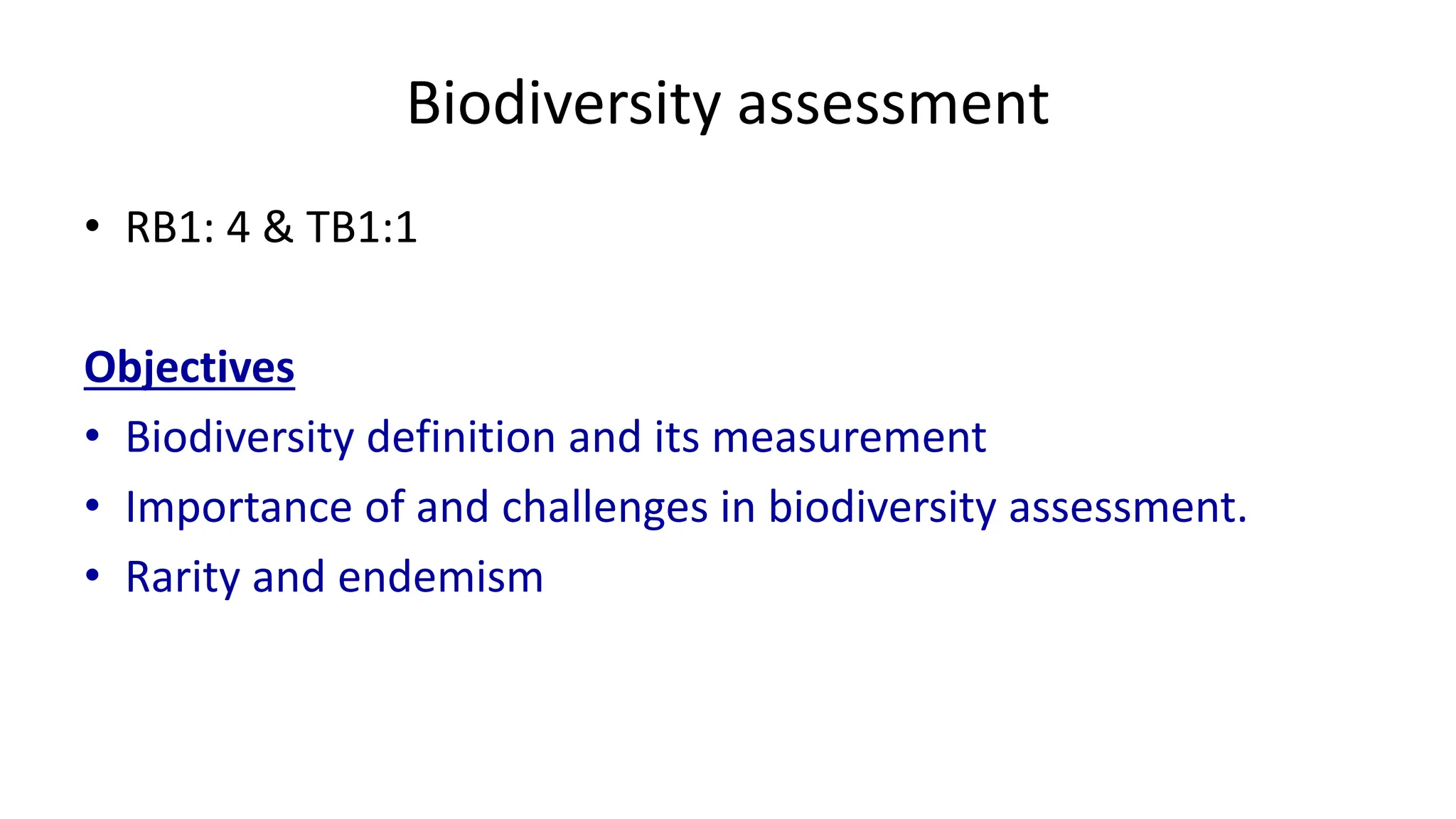
Biodiversity assessment
• RB1:4 & TB1:1
Objectives
• Biodiversity definition and its measurement
• Importance of and challenges in biodiversity assessment.
• Rarity and endemism
2.
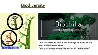
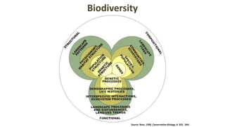
Biodiversity
"the connections thathuman beings subconsciously
seek with the rest of life.“
“the passionate love of life and of all that is alive.”
3.
• Measurable parameter
•WWF: millions of plants, animals & µorg., the genes they
contain and the intricate ecosys. they help to build into living
env.
Biodiversity indices
• Shannonindex: H = -Σpi*ln(pi)
• Simpson index: C = Σ(pi)2
• Probablity of interspecific encounter: PIE’ = 1- C
• Hills diversity index: N1 = e[H]
• Margalef: D= (S-1)/ln(N); S: # spp, N: # individuals in sample
Assumptions:
All individuals are randomly sampled
Population is indefinitely large, or effectively infinite
All species in the community are represented
15.
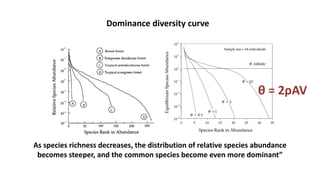
As species richnessdecreases, the distribution of relative species abundance
becomes steeper, and the common species become even more dominant”
Dominance diversity curve
θ = 2ρAV
16.
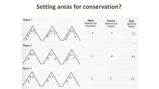
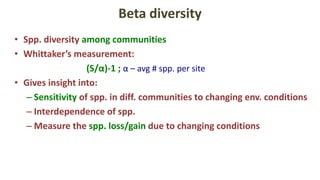
Beta diversity
• Spp.diversity among communities
• Whittaker’s measurement:
(S/α)-1 ; α – avg # spp. per site
• Gives insight into:
– Sensitivity of spp. in diff. communities to changing env. conditions
– Interdependence of spp.
– Measure the spp. loss/gain due to changing conditions
17.
Gamma diversity
• Productof α diversity of landscape communities and degree
of β differentiation among them
• (dS/dD)*[(g+l)/2]
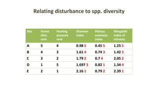
Relating disturbance tospp. diversity
Site Forest
distr.
rank
Hunting
pressure
rank
Shannon
index
Pielous
evenness
index
Margalafs
index of
richness
A 5 4 0.98 0.45 1.25
B 4 3 1.61 0.74 1.42
C 3 2 1.79 0.7 2.05
D 1 5 1.697 0.82 1.34
E 2 1 2.16 0.79 2.39
Site Forest
distr.
rank
Hunting
pressure
rank
Shannon
index
Pielous
evenness
index
Margalafs
index of
richness
A 5 4 0.98 5 0.45 5 1.25 5
B 4 3 1.61 4 0.74 3 1.42 3
C 3 2 1.79 2 0.7 4 2.05 2
D 1 5 1.697 3 0.82 1 1.34 4
E 2 1 2.16 1 0.79 2 2.39 1
20.
• High levelsof each leads to rarity
–α rarity
–β rarity
–γ rarity
21.
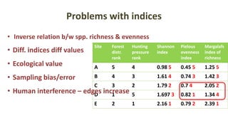
Problems with indices
•Inverse relation b/w spp. richness & evenness
Site Forest
distr.
rank
Hunting
pressure
rank
Shannon
index
Pielous
evenness
index
Margalafs
index of
richness
A 5 4 0.98 5 0.45 5 1.25 5
B 4 3 1.61 4 0.74 3 1.42 3
C 3 2 1.79 2 0.7 4 2.05 2
D 1 5 1.697 3 0.82 1 1.34 4
E 2 1 2.16 1 0.79 2 2.39 1
• Diff. indices diff values
• Ecological value
• Sampling bias/error
• Human interference – edges increase
22.
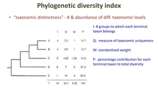
Phylogenetic diversity index
•“taxonomic distinctness” - # & abundance of diff. taxonomic levels
I: # groups to which each terminal
taxon belongs
Q: measure of taxonomic uniqueness
W: standardized weight
P: percentage contribution for each
terminal taxon to total diversity
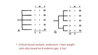
23.
• Critical faunalanalysis: endemism + taxic weight
rank sites based on # endemic gps. it has
I W P I W P
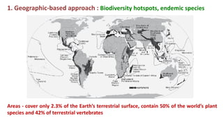
Areas - coveronly 2.3% of the Earth’s terrestrial surface, contain 50% of the world’s plant
species and 42% of terrestrial vertebrates
1. Geographic-based approach : Biodiversity hotspots, endemic species
27.
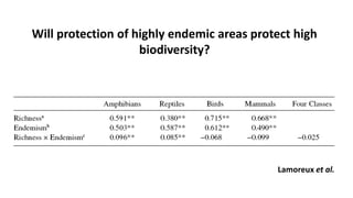
Lamoreux et al.
Willprotection of highly endemic areas protect high
biodiversity?


![Biodiversity indices
• Shannon index: H = -Σpi*ln(pi)
• Simpson index: C = Σ(pi)2
• Probablity of interspecific encounter: PIE’ = 1- C
• Hills diversity index: N1 = e[H]
• Margalef: D= (S-1)/ln(N); S: # spp, N: # individuals in sample
Assumptions:
All individuals are randomly sampled
Population is indefinitely large, or effectively infinite
All species in the community are represented](https://image.slidesharecdn.com/biodiversity-250304185002-cc74a986/85/Biodiversity-pdf-conservation-biology-course-14-320.jpg)
![Gamma diversity
• Product of α diversity of landscape communities and degree
of β differentiation among them
• (dS/dD)*[(g+l)/2]](https://image.slidesharecdn.com/biodiversity-250304185002-cc74a986/85/Biodiversity-pdf-conservation-biology-course-17-320.jpg)