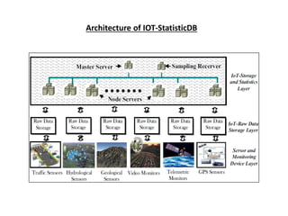
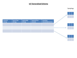
Big Data Mining and Internet of Things
Presented By-
Shubham Singh(40004796)
Shubhangi Sheel(40004793)
Problems
Paper 1: Data Mining with Big Data
 Modeling big data characteristics (HACE Theorem)
 Identify key challenges for big data mining
Paper 2: IOT-StatisticDB: A General Statistical Database Cluster Mechanism for Big Data
Analysis in the Internet of Things
 Sensor sampling data is huge, heterogeneous and have totally different formats and
semantics
 No statistical in database kernel analysis techniques available for IoT data
 Most of the existing statistical analysis methods are centralized solutions, unsuited forIoT
Kind of data we are talking about?
 Searching on Google with “Yan Mo Nobel Prize,” resulted in 1,050,000 web pointers
 News media
 Comments on social network
 Cross-referenced discussions by critics
 Square Kilometer Array (SKA) in radio astronomy consists of 1,000 to 1,500 dishes (15-meter)
in a central 5-km area in South Africa and Australia
 It provides 100 times more sensitive vision than any existing radio telescopes
 It generates 40 gigabytes (GB)/second data volume
 Existing methods can only work in an offline fashion and
are incapable of handling this Big Data scenario in real time
BIG DATA CHARACTERISTICS: HACE THEOREM
H: Heterogeneous
A: Autonomous Sources
C: Complex Data
E: Evolving Relationships
‘H’ for Heterogeneity
 Heterogeneous and diverse dimensionalities
 Different schemata and protocols
 Example: An individual is represented by
 Demographic Information: Text (gender, age , family disease history etc.)
 X-ray Examination: Image
 CT Scan: Image/ video
 DNA or genomic related test: Image (microarray expression images and sequences)
‘A’ for Autonomous sources with distributed and decentralized Control
 Autonomous data sources with distributed and decentralized controls
 Example: World Wide Web (WWW): Each web server provides a certain information
and is able to fully function independently
 Google, Flicker, Facebook, Walmart: Have large number of server farms deployed all
over the world
 Local legislations are different
 Seasonal promotions
 Top selling items
 Customer behavior
‘C’ for Complex Data and ‘E’ for Evolving Relationships
 In centralized information systems, the focus is on finding best feature values to represent
each observation
 Example: Facebook or Twitter
 An individual is represented by features but the social connections which is the most
important factor of human society is not taken into account
 In a dynamic world, the features evolve with respect to temporal, spatial, and other
factors.
Clustered data
Linear regression
Central core with 3 flaresLoopy behavior
Clustered data
DATA MINING CHALLENGES WITH BIG DATA
Tier III: Big Data Mining Algorithms
Tier II: Big Data Semantics and Application Knowledge
Tier I: Big Data Mining Platform
 A computing platform requires two resources: Hard disks and Processors
 Big data is distributed, so parallel computing and collective mining is used
 Frameworks rely on cluster computers with a high performance computing platforms such as
MapReduce or Enterprise Control Language
 Example: Super computer Titan, deployed at Oak Ridge National Laboratory in Tennessee,
contains 18,688 nodes each with a 16-core CPU.
Elephant in the room
Data Privacy
Tier II: Big Data Semantics and Application Knowledge
 Information Sharing and Data Privacy
 Restrict access to the data
 Anonymize data fields
 Domain and Application knowledge
 Identify right features for modeling the underlying data
 Example: Blood glucose level is clearly a better feature than body mass in diagnosing
Type II diabetes
Tier II: Big Data Semantics and Application Knowledge
Tier III: Big Data Mining Algorithms
 Local Learning and Model Fusion for Multiple Information Sources
 Mining distributed data often leads to biased view of the data resulting in biased
decisions or models
 To overcome this, we need to enable information exchange and fusion mechanisms to
ensure global optimization goal i.e. local mining and global correlations
Mining from Sparse, Uncertain, and Incomplete Data
Sparse, uncertain, and incomplete data are defining features for Big Data applications.
 Sparse data
 number of data points are too few for drawing reliable conclusions
 Uncertain data
 Data field is no longer deterministic but is subject to some
random/error distributions
 Data item is represented as sample distributions but not
as a single value, so most existing data mining algorithms
cannot be directly applied
 Incomplete data
 Incomplete data refers to the missing of data field values for
some samples
 Data imputation is an established research field that seeks
to impute missing values to produce improved models
Conclusion
 HACE theorem suggests that the key characteristics of the Big Data are
 Huge with heterogeneous and diverse data sources,
 Autonomous with distributed and decentralized control,
 Complex and Evolving in data and knowledge
 Analyzed several challenges at the data, model and system levels
 Analyzed challenges in Data mining:
 Information Sharing and Data Privacy
 Domain and Application knowledge
 Data Mining Algorithms
Paper 2: IOT-StatisticDB: A General Statistical Database Cluster Mechanism
for Big Data Analysis in the Internet of Things
This paper discusses :
 A generalized schemata to store different sensor data
 Distributed architecture for parallel computing for IoT
 Statistical analysis techniques and relevant operators
Architecture of IOT-StatisticDB
IoT Generalized Schema
SensorID
(String)
SensorType
(String)
DeployedBy
(String)
DepoyedTime
(Instant)
Samplings
(SamplingSequence)
Samplings
Definitions
1. Traffic Network: Net = (E, N)
I. E is set of e defined as the form e = (eid, geo, len, nids, nide)
II. N is set of n is defined as the form n = (nid, loc,(eid)m
i-1 ,mat)
III. Net = (E, N)
Node Region/ Service Area
IOT table and Data Distribution at IoT-Storage and Statistics Layer
2. SamplingValue = (t, loc, npos, schema, value)
* Note: Sampling value can be considered as a data type which defines the type of data from the sensors
3. SamplingComponent = (cSchema, cValue)
e.g. (“speed: real”, 62.5) or (“direction: real”, 22)
4. SamplingSequence = (schema, (ti, loci, nposi, valuei, flagi)n
i-1
Types of Sensors
Time (t) Location(loc)
Network
position(npos)
Schema Value
Temperature t1 39.5, 145.2 null “temperature: real” 27.5
GPS
t2
39.3, 144.3 e201
“speed: real, direction:
real”
(62.5, 22)
Wind
t3
38.2, 142.8 Null
“windspeed: real,
winddir: real”
(62.5, 22)
Vitalized value
from Traffic
Video Camera
t4
39.7, 142.1 e202
“averageSpeed: real,
jam: bool”
(62.5, true)
Query Operators for Data Retrieval and for Statistical Analysis
*Format: FunctionName (Input Parameters) -> Output
Truncation Operators:
1. truncateGeo (SamplingSequence*Region) ->SamplingSequence
2. truncateTime (SamplingSequence*Periods)->SamplingSequence
3. atInstant (SamplingSequence* Instant )-> SamplingValue
Types of Sensors
Time (t) Location(loc)
Network
position(npos)
Schema Value
Temperature t1 39.5, 145.2 null “temperature: real” 27.5
GPS
t2
39.3, 144.3 e201
“speed: real, direction:
real”
(62.5, 22)
Wind
t3
38.2, 142.8 Null
“windspeed: real,
winddir: real”
(62.5, 22)
Vitalized value
from Traffic
Video Camera
t4
39.7, 142.1 e202
“averageSpeed: real,
jam: bool”
(62.5, true)
Projection Operators:
Component Extraction Operator:
getComponent: SamplingValue*integer -> SamplingComponent
Statistical Analysis Operators
spatialAggrEU: String *String -> Region
spatialAggrNet: String* String-> Lines
parameterAggrEU: String*String-> Real
parameterAggrNet: String *String-> Set(String *String)
Sampling-Sequence-Based Projections Sampling-Value-Based Projections
sProjectLines: SamplingSequence -> Lines //for moving sensors
sProjectPoint: SamplingSequence -> Point //for static sensors
sProjectNetPos: SamplingSequence->Set(String)
sProjectTime: SamplingSequence -> Periods
vProjectPoint: SamplingValue-> Point
vProjectNetPos: SamplingValue-> String
vProjectTime: SamplingValue -> Instant
Euclidean-Based Spatial Aggregation
Q1: If the task is to find area in BeijingGeo where the pollution level is above 450 at time t.
Qdata = “SELECT sProjectPoint(Samplings) FROM IoTData
WHERE SensorType = “PollutionSensor”
AND inside(sProjectPoint(Samplings), BeijingGeo)
AND getComponent(atInstant(Samplings, t), 1) > 450”;
Select spatialAggrEU (Qdata, DBScan (distance1, number1))
Algorithm:
INPUT: Qdata: String; // Statistical raw data collection query
cMethodPara: String;
// Clustering method and its parameters;
OUTPUT: R: Region;
1. queryRegion = GetQueryRange(Qdata);
2. Nodes = {node | area(node) queryRegion Ø}
3. FOR node Nodes DO IN PARALLEL
4. StatisticalRawData = Execute(Qdata);
5. R (node) = clusterContour(StatisticalRawData, cMethodPara);
6. SendMaster(R (node));
7. ENDFOR;
8. Results = {R(node) | node Nodes};
9. R = regionMerge(Results);
10. Return (R).
Network-Based Spatial Aggregation
Q2: If task is to find area blocked edge sections with vehicle speed lower than 5 km/h) at time t in the
traffic network of Beijing area
Qdata = “SELECT atInstant(Samplings, t)
FROM IoTData
WHERE SensorType = “VehicleGPS”
AND inside(sProjectPoint (atInstant(Samplings, t)), BeijingGeo)
AND getComponent(atInstant(Samplings, t), 1) < 5”;
Select spatialAggrNet (Qdata, DBScanNet(distance1, number1))
Algorithm:
INPUT: Qdata: String; //Raw data collection query
cMethodPara:String; //clustering method& parameters;
TrafficNet: Net; //the traffic network;
OUTPUT: R: Lines;
1. queryRegion = GetQueryRange(Qdata);
2. Nodes = {node | area(node) queryRegion Ø}
3. FOR node Nodes DO IN PARALLEL
4. StatisticalRawData = Execute(Qdata);
5. R (node) = netClusterLines(StatisticalRawData, trafficNet, cMethodPara);
6. SendMaster(R(node));
7. ENDFOR;
8. Results = {R(node) | node Nodes};
9. R = linesMerge(Results);
10. Return (R).
Euclidean-based Parameter Aggregation
Q3: If task is to find the average pollution level at time t in BeijingGeo.
Qdata=“SELECT getComponent(atInstant(Samplings, t), 1)
FROM IoTData
WHERE SensorType = “PollutionSensor”
AND inside(sProjectPoint(Samplings), BeijingGeo)”;
Select parameterAggrEU (Qdata, Average)
Algorithm:
INPUT: Qdata: String; //Raw data collection query
method: String; //aggregation method
OUTPUT: R: Real;
1. queryRegion = GetQueryRange(Qdata);
2. Nodes = {node | area(node) queryRegion Ø}
3. FOR node Nodes DO IN PARALLEL
4. StatisticalRawData = Execute(Qdata);
5. R (node) = aggregate(StatisticalRawData, method);
6. N (node) = |StatisticalRawData|;
7. SendMaster(R(node), N(node));
8. ENDFOR;
9. Results = {(R(node), N(node)) | node Nodes};
10. R = valueMerge(Results, method);
11. Return (R).
Network-based Parameter Aggregation
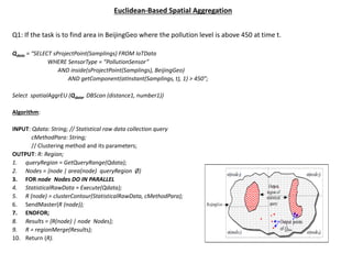
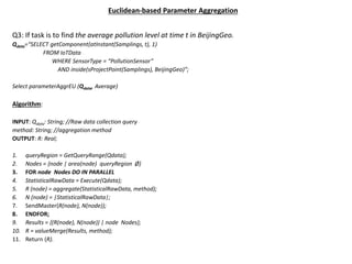
Q4: If task is to find the traffic flow parameters at time t for each edge in BeijingGeo.
Qdata= “SELECT sTruncateTime(sTruncateGeo (Samplings, BeijingGeo), [ t - 5*Minute, t ])
FROM IoTData
WHERE SensorType = “VehicleGPS””
Select parameterAggrNet (Qdata, TrajectoryAnalysis);
Algorithm:
INPUT: Qdata:String; //Raw data collection query
method: String; //aggregation method
OUTPUT: R; //of the form Set((edgeID:string, para: string))
1. queryRegion = GetQueryRange(Qdata);
2. Nodes = {node | area(node) queryRegion Ø}
3. FOR node Nodes DO IN PARALLEL
4. StatisticalRawData = Execute(Qdata);
5. R (node) = trafficAnalysis(StatisticalRawData, method);
6. SendMaster(R (node));
7. ENDFOR;
8. Results = {R(node) | node Nodes};
9. R = edgeBasedValueMerge(Results);
10. Return (R).
Experimental Studies
 The prototype system contained one master server and 2~32 node servers.
 The real GPS trajectory data was collected from 20,000 taxi cabs in Beijing and the
average GPS sampling frequency was 30 seconds.
 The sampling sequence data of 200,000 static sensors was generated through simulation
and the average sampling frequency of static sensors was 5 minutes.
 Compared with: Centralized Statistical Analysis with Data Source Distributed (CSA-DSD): It
stores sensor sampling data in a distributed manner among multiple node servers but has
one master server to do all the statistical analysis
 We performed above 4 queries on both IoT and CSA-DSD and compare the query time
response against numbers of nodes and number of sensors.
Query response time vs. number of nodes
Query response time vs. no. of sensors
Conclusions
 A generalized schemata to store different sensor data was proposed
 Proposed architecture to store data in distributed manner and parallel computing in real time
basis
 Statistical analysis operators were defined
 Algorithms for statistical analysis of IoT data was proposed.
 Experimental results were compared with other similar framework.
Big Data and IOT

Big Data and IOT

  • 1.
    Big Data Miningand Internet of Things Presented By- Shubham Singh(40004796) Shubhangi Sheel(40004793)
  • 9.
    Problems Paper 1: DataMining with Big Data  Modeling big data characteristics (HACE Theorem)  Identify key challenges for big data mining Paper 2: IOT-StatisticDB: A General Statistical Database Cluster Mechanism for Big Data Analysis in the Internet of Things  Sensor sampling data is huge, heterogeneous and have totally different formats and semantics  No statistical in database kernel analysis techniques available for IoT data  Most of the existing statistical analysis methods are centralized solutions, unsuited forIoT
  • 10.
    Kind of datawe are talking about?  Searching on Google with “Yan Mo Nobel Prize,” resulted in 1,050,000 web pointers  News media  Comments on social network  Cross-referenced discussions by critics  Square Kilometer Array (SKA) in radio astronomy consists of 1,000 to 1,500 dishes (15-meter) in a central 5-km area in South Africa and Australia  It provides 100 times more sensitive vision than any existing radio telescopes  It generates 40 gigabytes (GB)/second data volume  Existing methods can only work in an offline fashion and are incapable of handling this Big Data scenario in real time
  • 11.
    BIG DATA CHARACTERISTICS:HACE THEOREM H: Heterogeneous A: Autonomous Sources C: Complex Data E: Evolving Relationships
  • 12.
    ‘H’ for Heterogeneity Heterogeneous and diverse dimensionalities  Different schemata and protocols  Example: An individual is represented by  Demographic Information: Text (gender, age , family disease history etc.)  X-ray Examination: Image  CT Scan: Image/ video  DNA or genomic related test: Image (microarray expression images and sequences)
  • 13.
    ‘A’ for Autonomoussources with distributed and decentralized Control  Autonomous data sources with distributed and decentralized controls  Example: World Wide Web (WWW): Each web server provides a certain information and is able to fully function independently  Google, Flicker, Facebook, Walmart: Have large number of server farms deployed all over the world  Local legislations are different  Seasonal promotions  Top selling items  Customer behavior
  • 14.
    ‘C’ for ComplexData and ‘E’ for Evolving Relationships  In centralized information systems, the focus is on finding best feature values to represent each observation  Example: Facebook or Twitter  An individual is represented by features but the social connections which is the most important factor of human society is not taken into account  In a dynamic world, the features evolve with respect to temporal, spatial, and other factors.
  • 15.
    Clustered data Linear regression Centralcore with 3 flaresLoopy behavior Clustered data
  • 16.
  • 17.
    DATA MINING CHALLENGESWITH BIG DATA Tier III: Big Data Mining Algorithms Tier II: Big Data Semantics and Application Knowledge Tier I: Big Data Mining Platform
  • 18.
    Tier I: BigData Mining Platform  A computing platform requires two resources: Hard disks and Processors  Big data is distributed, so parallel computing and collective mining is used  Frameworks rely on cluster computers with a high performance computing platforms such as MapReduce or Enterprise Control Language  Example: Super computer Titan, deployed at Oak Ridge National Laboratory in Tennessee, contains 18,688 nodes each with a 16-core CPU.
  • 19.
  • 20.
  • 21.
    Tier II: BigData Semantics and Application Knowledge  Information Sharing and Data Privacy  Restrict access to the data  Anonymize data fields
  • 22.
     Domain andApplication knowledge  Identify right features for modeling the underlying data  Example: Blood glucose level is clearly a better feature than body mass in diagnosing Type II diabetes Tier II: Big Data Semantics and Application Knowledge
  • 23.
    Tier III: BigData Mining Algorithms  Local Learning and Model Fusion for Multiple Information Sources  Mining distributed data often leads to biased view of the data resulting in biased decisions or models  To overcome this, we need to enable information exchange and fusion mechanisms to ensure global optimization goal i.e. local mining and global correlations
  • 24.
    Mining from Sparse,Uncertain, and Incomplete Data Sparse, uncertain, and incomplete data are defining features for Big Data applications.  Sparse data  number of data points are too few for drawing reliable conclusions  Uncertain data  Data field is no longer deterministic but is subject to some random/error distributions  Data item is represented as sample distributions but not as a single value, so most existing data mining algorithms cannot be directly applied  Incomplete data  Incomplete data refers to the missing of data field values for some samples  Data imputation is an established research field that seeks to impute missing values to produce improved models
  • 25.
    Conclusion  HACE theoremsuggests that the key characteristics of the Big Data are  Huge with heterogeneous and diverse data sources,  Autonomous with distributed and decentralized control,  Complex and Evolving in data and knowledge  Analyzed several challenges at the data, model and system levels  Analyzed challenges in Data mining:  Information Sharing and Data Privacy  Domain and Application knowledge  Data Mining Algorithms
  • 27.
    Paper 2: IOT-StatisticDB:A General Statistical Database Cluster Mechanism for Big Data Analysis in the Internet of Things This paper discusses :  A generalized schemata to store different sensor data  Distributed architecture for parallel computing for IoT  Statistical analysis techniques and relevant operators
  • 28.
  • 29.
  • 30.
    Definitions 1. Traffic Network:Net = (E, N) I. E is set of e defined as the form e = (eid, geo, len, nids, nide) II. N is set of n is defined as the form n = (nid, loc,(eid)m i-1 ,mat) III. Net = (E, N) Node Region/ Service Area
  • 31.
    IOT table andData Distribution at IoT-Storage and Statistics Layer
  • 32.
    2. SamplingValue =(t, loc, npos, schema, value) * Note: Sampling value can be considered as a data type which defines the type of data from the sensors 3. SamplingComponent = (cSchema, cValue) e.g. (“speed: real”, 62.5) or (“direction: real”, 22) 4. SamplingSequence = (schema, (ti, loci, nposi, valuei, flagi)n i-1 Types of Sensors Time (t) Location(loc) Network position(npos) Schema Value Temperature t1 39.5, 145.2 null “temperature: real” 27.5 GPS t2 39.3, 144.3 e201 “speed: real, direction: real” (62.5, 22) Wind t3 38.2, 142.8 Null “windspeed: real, winddir: real” (62.5, 22) Vitalized value from Traffic Video Camera t4 39.7, 142.1 e202 “averageSpeed: real, jam: bool” (62.5, true)
  • 33.
    Query Operators forData Retrieval and for Statistical Analysis *Format: FunctionName (Input Parameters) -> Output Truncation Operators: 1. truncateGeo (SamplingSequence*Region) ->SamplingSequence 2. truncateTime (SamplingSequence*Periods)->SamplingSequence 3. atInstant (SamplingSequence* Instant )-> SamplingValue Types of Sensors Time (t) Location(loc) Network position(npos) Schema Value Temperature t1 39.5, 145.2 null “temperature: real” 27.5 GPS t2 39.3, 144.3 e201 “speed: real, direction: real” (62.5, 22) Wind t3 38.2, 142.8 Null “windspeed: real, winddir: real” (62.5, 22) Vitalized value from Traffic Video Camera t4 39.7, 142.1 e202 “averageSpeed: real, jam: bool” (62.5, true)
  • 34.
    Projection Operators: Component ExtractionOperator: getComponent: SamplingValue*integer -> SamplingComponent Statistical Analysis Operators spatialAggrEU: String *String -> Region spatialAggrNet: String* String-> Lines parameterAggrEU: String*String-> Real parameterAggrNet: String *String-> Set(String *String) Sampling-Sequence-Based Projections Sampling-Value-Based Projections sProjectLines: SamplingSequence -> Lines //for moving sensors sProjectPoint: SamplingSequence -> Point //for static sensors sProjectNetPos: SamplingSequence->Set(String) sProjectTime: SamplingSequence -> Periods vProjectPoint: SamplingValue-> Point vProjectNetPos: SamplingValue-> String vProjectTime: SamplingValue -> Instant
  • 35.
    Euclidean-Based Spatial Aggregation Q1:If the task is to find area in BeijingGeo where the pollution level is above 450 at time t. Qdata = “SELECT sProjectPoint(Samplings) FROM IoTData WHERE SensorType = “PollutionSensor” AND inside(sProjectPoint(Samplings), BeijingGeo) AND getComponent(atInstant(Samplings, t), 1) > 450”; Select spatialAggrEU (Qdata, DBScan (distance1, number1)) Algorithm: INPUT: Qdata: String; // Statistical raw data collection query cMethodPara: String; // Clustering method and its parameters; OUTPUT: R: Region; 1. queryRegion = GetQueryRange(Qdata); 2. Nodes = {node | area(node) queryRegion Ø} 3. FOR node Nodes DO IN PARALLEL 4. StatisticalRawData = Execute(Qdata); 5. R (node) = clusterContour(StatisticalRawData, cMethodPara); 6. SendMaster(R (node)); 7. ENDFOR; 8. Results = {R(node) | node Nodes}; 9. R = regionMerge(Results); 10. Return (R).
  • 36.
    Network-Based Spatial Aggregation Q2:If task is to find area blocked edge sections with vehicle speed lower than 5 km/h) at time t in the traffic network of Beijing area Qdata = “SELECT atInstant(Samplings, t) FROM IoTData WHERE SensorType = “VehicleGPS” AND inside(sProjectPoint (atInstant(Samplings, t)), BeijingGeo) AND getComponent(atInstant(Samplings, t), 1) < 5”; Select spatialAggrNet (Qdata, DBScanNet(distance1, number1)) Algorithm: INPUT: Qdata: String; //Raw data collection query cMethodPara:String; //clustering method& parameters; TrafficNet: Net; //the traffic network; OUTPUT: R: Lines; 1. queryRegion = GetQueryRange(Qdata); 2. Nodes = {node | area(node) queryRegion Ø} 3. FOR node Nodes DO IN PARALLEL 4. StatisticalRawData = Execute(Qdata); 5. R (node) = netClusterLines(StatisticalRawData, trafficNet, cMethodPara); 6. SendMaster(R(node)); 7. ENDFOR; 8. Results = {R(node) | node Nodes}; 9. R = linesMerge(Results); 10. Return (R).
  • 37.
    Euclidean-based Parameter Aggregation Q3:If task is to find the average pollution level at time t in BeijingGeo. Qdata=“SELECT getComponent(atInstant(Samplings, t), 1) FROM IoTData WHERE SensorType = “PollutionSensor” AND inside(sProjectPoint(Samplings), BeijingGeo)”; Select parameterAggrEU (Qdata, Average) Algorithm: INPUT: Qdata: String; //Raw data collection query method: String; //aggregation method OUTPUT: R: Real; 1. queryRegion = GetQueryRange(Qdata); 2. Nodes = {node | area(node) queryRegion Ø} 3. FOR node Nodes DO IN PARALLEL 4. StatisticalRawData = Execute(Qdata); 5. R (node) = aggregate(StatisticalRawData, method); 6. N (node) = |StatisticalRawData|; 7. SendMaster(R(node), N(node)); 8. ENDFOR; 9. Results = {(R(node), N(node)) | node Nodes}; 10. R = valueMerge(Results, method); 11. Return (R).
  • 38.
    Network-based Parameter Aggregation Q4:If task is to find the traffic flow parameters at time t for each edge in BeijingGeo. Qdata= “SELECT sTruncateTime(sTruncateGeo (Samplings, BeijingGeo), [ t - 5*Minute, t ]) FROM IoTData WHERE SensorType = “VehicleGPS”” Select parameterAggrNet (Qdata, TrajectoryAnalysis); Algorithm: INPUT: Qdata:String; //Raw data collection query method: String; //aggregation method OUTPUT: R; //of the form Set((edgeID:string, para: string)) 1. queryRegion = GetQueryRange(Qdata); 2. Nodes = {node | area(node) queryRegion Ø} 3. FOR node Nodes DO IN PARALLEL 4. StatisticalRawData = Execute(Qdata); 5. R (node) = trafficAnalysis(StatisticalRawData, method); 6. SendMaster(R (node)); 7. ENDFOR; 8. Results = {R(node) | node Nodes}; 9. R = edgeBasedValueMerge(Results); 10. Return (R).
  • 39.
    Experimental Studies  Theprototype system contained one master server and 2~32 node servers.  The real GPS trajectory data was collected from 20,000 taxi cabs in Beijing and the average GPS sampling frequency was 30 seconds.  The sampling sequence data of 200,000 static sensors was generated through simulation and the average sampling frequency of static sensors was 5 minutes.  Compared with: Centralized Statistical Analysis with Data Source Distributed (CSA-DSD): It stores sensor sampling data in a distributed manner among multiple node servers but has one master server to do all the statistical analysis  We performed above 4 queries on both IoT and CSA-DSD and compare the query time response against numbers of nodes and number of sensors.
  • 40.
    Query response timevs. number of nodes
  • 41.
    Query response timevs. no. of sensors
  • 42.
    Conclusions  A generalizedschemata to store different sensor data was proposed  Proposed architecture to store data in distributed manner and parallel computing in real time basis  Statistical analysis operators were defined  Algorithms for statistical analysis of IoT data was proposed.  Experimental results were compared with other similar framework.